Добавил:

Upload Опубликованный материал нарушает ваши авторские права? Сообщите нам.

Вуз:

Санкт-Петербургский государственный университет

Предмет:

Файл:

01_Rider_po_kursu_itogovyy_variant / Тема 12. Партии и политическая дифференциация населения / Evolution of Party Systim....AJPS. 2003. Vol. 47. No 2.doc

Скачиваний:

Добавлен:

16.04.2015

Размер:

436.74 Кб

Скачать

☆

1 / 31 2 3 > Следующая >>>

_STOR

The Evolution of Party Systems between Elections

Michael Laver; Kenneth Benoit

American Journal of Political Science, Vol. 47, No. 2. (Apr., 2003), pp. 215-233.

Stable URL: http://links.jstor.org/sici?sici=0092-5853%28200304%2947%3A2%3C215%3ATEOPSB%3E2.0.CO%3B2-L

American Journal of Political Science is currently published by Midwest Political Science Association.

Your use of the JSTOR archive indicates your acceptance of JSTOR's Terms and Conditions of Use, available at http://www.jstor.org/about/terms.html. JSTOR's Terms and Conditions of Use provides, in part, that unless you have obtained prior permission, you may not download an entire issue of a journal or multiple copies of articles, and you may use content in the JSTOR archive only for your personal, non-commercial use.

Please contact the publisher regarding any further use of this work. Publisher contact information may be obtained at http://www.jstor.org/journals/mpsa.html.

Each copy of any part of a JSTOR transmission must contain the same copyright notice that appears on the screen or printed page of such transmission.

JSTOR is an independent not-for-profit organization dedicated to and preserving a digital archive of scholarly journals. Formore information regarding JSTOR, please contact support@jstor.org.

http://www.jstor.org Sat Feb 17 04:38:36 2007

^{The Evolution of Party
Systems between Elections}

Michael Laver Trinity College Kenneth Benoit Trinity College

Most existing theoretical work on party competition pays little attention to the evolution of party systems between elections as a result of defections between parties. In this article, we treat individual legislators as utility-maximizing agents tempted to defect to other parties if this would increase their expected payoffs. We model the evolution of party systems between elections in these terms and discuss this analytically, exploring unanswered questions using computational methods. Under office-seeking motivational assumptions, our results strikingly highlight the role of the largest party, especially when it is "dominant" in the technical sense, as a pole of attraction in interelectoral evolution.

The existing political science account of party competition pays little attention to the evolution of legislatures between elections, despite the fact that, in all real legislatures, there is a great deal of politics between elections. In particular, legislators may defect from one party and join another, parties may split and fuse, and the party system may thereby evolve into one quite different from that produced by the election result. This carries obvious analytical implications for modeling party competition and important normative implications for our appreciation of representative democracy. In supplying the link between the popular mandate and public policy in representative democracy, the forces that shape legislatures between elections are clearly very important.

While there is a literature on party switching in the U.S. Congress (e.g., Nokken 2000), exploration of this in other contexts is very limited. Yet it is precisely in multiparty systems that the phenomenon is most prevalent and important. In the Italian legislature between 1996 and spring 2000, for instance, more than one in four deputies changed parties at least once (Heller and Mershon 2001, 2). Similar patterns of party switching can be seen in Japan (Laver and Kato, 2001), Poland (Benoit and Hayden 2001), and elsewhere (see Bowler, Farrell, and Katz 1999). At present there is very little work modeling this process in a multiparty context. Existing studies focus on party discipline (Heller and Mershon 2001), the electoral connection

(Heller and Mershon 2001; de Dios 2001), or problems of party consolidation (Agh 1999; Verzichelli 1999). Every defection from some party, however, implies that some other party is willing to accept the defector. Existing work on party switching focuses exclusively on the rationale of the switchers, while ignoring the incentives of the parties that the switchers are attempting to join. Finally, existing models have nothing to say as to which party switchers will wish to join when there are several possibilities.

Absent from the literature on party switching is any consideration of the payoffs that politicians expect from affiliation to a given legislative party. Yet, in addition to the electoral benefits of a party label, membership of a legislative party is the key to many of the payoffs of "winning" the political game by getting into office and being associated with the incumbent government, as Cox (1987) pointed out in his analysis of the evolution of coherent political parties in Britain. Even in countries such as Britain or Ireland where the electoral system makes it possible to be returned to parliament as an "independent" without party affiliation, it is effectively impossible for an independent legislator to enter government.

Here we model the party affiliation of legislators as a matter of choice that is continuously under review. We explore ways in which some parties attract potential defectors, some are willing to accept defectors, and some are both attractive and willing, allowing defections actually to take place. Rather than seeing the legislative party

Michael Laver is Professor of Political Science at Trinity College, University of Dublin, Dept. of Political Science, Dublin 2, Ireland (mlaver@tcd.ie). Kenneth Benoit is Lecturer in Political Science at Trinity College, University of Dublin, Dept. of Political Science, Dublin 2, Ireland (kbenoit@tcd.ie).

We thank Kenneth Shepsle, Patrick Dunleavy, Steven Reed, Thomas Brauninger, and three anonymous referees for comments. Work on this article was carried out while Michael Laver was a Government of Ireland Senior Research Fellow.

ISSN 0092-5853

215

216

MICHAEL LAYER AND KENNETH BENOIT

system as remaining static between elections, we treat the composition of legislative parties as the output of one cycle in the process of legislative politics, as well as an input into the next cycle. In this way, we explore the evolution of legislative party systems between elections and provide insights into the structure and stability of different types of party system. We describe our approach to analyzing the evolution of legislative party systems between elections in the second section. In the third section we explore analytically some of the implications of this approach for party competition. In the fourth section we continue this exploration using computational methods to investigate the comparative statics of our model. In the fifth section we characterize what makes certain parties "attractive" to, and "willing" to accept, defectors. We conclude in the sixth section with a review of the substantive implications of these results for multiparty systems, with special reference to the bases of competition between the two largest parties.

Analyzing the Evolution of Party Systems between Elections

Most models of government formation and party competition describe a system in which nothing happens in a legislature between elections, except perhaps reactions to a stream of exogenous shocks.¹ Our focus, in contrast, is precisely upon moves made by legislators between elections. We envisage a process in which legislators continuously keep their party affiliation under review, being attracted to defect to other parties if these offer higher payoffs.

Members of existing parties are willing to accept new members if this enhances their own expectations. Each time a legislator changes party affiliation there is a new party configuration. All legislators then reconsider their position since their expected payoffs will have changed. Thus each change in affiliation potentially provokes another, unless an equilibrium is reached in which no legislator who wants to change parties can find a party he both wants to join and that is willing to accept a new member. What we construct below is a model of legislative rather than electoral politics. In an ideal world we would construct a model that took account of the interaction between legislative, executive, and electoral politics. We feel we would set ourselves an impossible analytical task if we tried to do this at the outset, however, and thus concen-

¹ For work modeling reactions in a legislature to exogenous shocks, see Lupia and Strom (1995); Laver and Shepsle (1998); Diermeier and Stevenson (1999, 2000); Diermeier and Merlo (2000).

trate on the legislative arena, accepting that this is only part of the story.

Motivational Assumptions

Many types of payoff motivate politicians to join legislative parties. In the existing literature, payoffs are divided into two classes, one focused on the benefits of office and the other on policy. Office-seeking models assume that the paramount objective of legislators is to get into office (e.g., Downs 1957), and that features such as policy positions are essentially instrumental. Policy-seeking models, in contrast, are grounded in the assumption that policy outputs rather than the perquisites of office provide the fundamental political payoffs (e.g., McKelvey and Schofield 1986,1987).Most authors recognize thatamore realistic model would combine both office- and policy-seeking motivations, but there is no basic agreement on the rather arbitrary trade-offs between office and policy payoffs that such models require. Nor it is clear that such models could be solved or even clearly specified.

Our approach is deliberately simple. We focus on the office-seeking payoffs to members of a party that goes into government, defined as a party that nominates members of the cabinet. Nonetheless, when we discuss the analytical implications of our model, we give some consideration to the effects on our conclusions of assuming alternative, policy-seeking motivations.

Operationalizing Office-Seeking Expectations

Within the government formation literature and following Riker (1962), office-seeking motivations are conceived in terms of competition for a fixed set of rewards of office. The expected collective payoff, or expectation, of a set of legislators forming a Party P in a given party configuration, D, is thus Е_рд, defined on the interval [0,1] as their expected collective share of the total fixed payoff.

Going beyond the unitary actor approach, we must make an assumption about how much a legislator expects to receive from any party to which he belongs. The sparest assumption uses no information about intraparty factions or decision making. All legislators are seen as autonomous actors. In the intraparty politics that distributes the spoils of victory, all legislators are assumed to be equivalent— by symmetry, all have equal expectations. The expectation of a generic legislator L in Party P with a seat share s_p in configuration D is thus E_ptj/s_p. This measure of the expectation of a generic party legislator is the "expectation-to-weight" ratio (EWR) of the party in question.

THE EVOLUTION OF PARTY SYSTEMS BETWEEN ELECTIONS

217

Note that if we had information about factional structures, the substantive roles of individual legislators or other aspects of intraparty politics, we might want to model intraparty resource allocation in a different way and would then need more complex indicators of the expectations of legislators. For example, if we had information on intraparty factions and an intraparty decision rule, then we could model intraparty bargaining and estimate the payoff to each faction. For example a "seniority" rule that gave longer-affiliated legislators a higher share of party payoffs than new party members might reduce the incentives of legislators to defect if they anticipate future rewards for their present loyalty. This is an interesting matter to which we will return in future work but we note here that, if intraparty resource allocation gives some legislator an above average expectation, then it must give another in the same party a below average expectation. Thus our assumption about the expectations of individual legislators is conservative in the sense that, once defection from a party is rational for a legislator of average expectation, E_p<i/sp, then it will always be rational for some legislator in that party.

We now operationalize our assumption about expected payoffs in a party system populated by office-seeking actors. We think of the set of expectations of each party in a given party configuration as that configuration's expectation vector. Here, we operationalize expectations by assuming that the expected payoff of Party P in configuration D, E_pj, is proportional to Party P's constant-sum bargaining power within that configuration of parties. This allows us to use an index of bargaining expectations in an office-seeking coalition system, such as the Shapley-Shubik index (or indeed any of many others that have subsequently been devised). This index is both widely used within the profession and mathematically elegant. It measures expectations in terms of the extent that a given actor is pivotal in the coalition formation process, in the sense of turning a losing coalition into a winning one by joining it, or turning a winning coalition into a losing one by leaving it. Despite its many subsequent uses and misuses, the original core interpretation of the Shapley-Shubik index was indeed in terms of bargaining expectations (see especially Shapley 1953). It is vital to keep this firmly in mind in the present context, because the index is not used here as an arbitrary number estimating a particular type of a priori voting power.² It is instead used in its original sense as an operationaliza-

² For a recent heated debate on the appropriateness of using power indices to model voting power in the EU, see Garrett and Tsebelis (1999); Holler and Widgren (1999); Lane and Berg (1999); Nurmi and Meskanen (1999); Lane and Maeland (2000).

tion of the incentive structure of an office-seeking party system.³

Modeling the Evolutionary Dynamics of Party Switching

The basic structure of the process we envisage is as follows.

Stage 1: A legislative election is held. For the reasons we discuss above, we treat this as an unmodeled discontinuity in the process we describe. The election result determines the identity of m politicians who form the legislature and partitions these into n legislative parties. This partition is the starting configuration for a process of evolution between elections.

Stage 2: Some legislator L in some Party P is activated to consider whether to defect from one party and join another. We can think of this activation as arising from a random "personal event"—perhaps a fight with party colleagues, an external shock to the environment, an individual personal development. Other legislators have no information about the personal event history and future of legislator I and cannot predict when and in what context L will be activated. We say I is attracted to another party, Q, and that Q is attractive to I, if I expects to receive higher payoffs as a result of defecting from P to Q. Individual members of Party Q will only be willing to accept L as a new member, however, if this increases their own expected payoffs. Legislator L thus scans all other parties in order of attractiveness—that is, in order of the expected payoff to L if L joins the party concerned. I identifies the most attractive party, the members of which are also willing to accept I as a new member.⁴

Stage 3: Legislator L defects to, and is accepted by the members of, the most attractive willing alternative party he or she can find, if an attractive willing alternative exists. If no attractive willing alternative exists, L stays put. If L changes parties, the system evolves into a new partition of m politicians into n parties, unless some party disappears completely as a result of the defection. If L does not change, the system remains static.

Stage 4: Stages 2 and 3 are repeated continuously unless an election intervenes and generates a new legislature, returning the process to Stage 1.

³In a recent extensive review of the uses and abuses of power indices Felsenthal and Machover (2001, 86) argue that, from a technical point of view, the Shapley-Shubik index deals with what they call P-power, "a voter's relative share in some prize, which a winning coalition can put its hands on by the very act of winning."

⁴ It is theoretically possible for a legislator to defect to form a one-person party. We do not consider defections to "independent" status here for the reasons discussed in the opening section.

218

MICHAEL LAYER AND KENNETH BENOIT

In the context of the process described above, consider a party configuration D and a generic legislator I affiliated to a Party P that controls a share s_p of the seats. The relative expectations of the legislator arising from either staying in Party P or defecting to some other Party Q are as follows:

Expectation arising from staying in Party P: = E_pj/s_p

(1.1) Expectation arising from defecting to Party Q:

E iaiIs ' (I 2)
^qd/^q V¹*^-/

where q',s', and d' relate to the party being joined, its seat share and the party configuration, as these stand after the defection.

A generic legislator in Party P has an incentive to defect to Party Q if:

P , ,,/c , > P ,lc (J 1\

ⁱ-¹ q a /^Jq ^±-'pa/^Jp y^"¹-/

If condition 2.1 is satisfied, then Party Q will be attractive to a generic legislator I in Party P. The expectations of I are enhanced by defecting from P and joining Q. It is not enough, however, for some legislator to want to defect to another party. Members of the receiving party must also accept defections. Generic members of Party Q will be willing to accept a defector if:

That is, the accepting party's expectation-to-weight ratio (EWR), and hence the expectations of a generic member, must increase as a result of accepting the defector. Note crucially that, since a party's weight always increases as a result of accepting a defection, this also means that a party's absolute expectation must increase, and hence the expectation vector must change, before its members are likely to accept a defector.

If, for some P, Party Q satisfies both 2.1 and 2.2, then Q will attract, and its members will be willing to accept, defections from P and the system will evolve. If, for every P, there is no Q that satisfies both 2.1 and 2.2, then the system will not evolve and will appear to be in a static equilibrium.

Analytical Implications of the Model

We now use our model to derive propositions that yield insights into the evolution of party competition between elections. Our model is not game-theoretic in the classical sense, since we do not assume that legislators solve the entire complex dynamic game that describes the day-by-day evolution of a legislature and then each make the perfect

first move. The game tree is explosive and the problem hardly more tractable than that of solving for equilibrium strategies in a game of chess. Rather we assume that legislators adapt to changes in the party system as these unfold. In this sense our approach has more in common with evolutionary game theory or artificial life models than with classical game theory (see, for example, Axelrod 1997; Axelrod and Cohen 2000; Skyrms 1996). Our approach relies on an iterated adaptive decision theoretic framework wherein the utility of individual legislators is defined by conditions that evolve with each iteration of the game. Furthermore, because a stochastic function selects individual legislators for activation, the framework is not deterministic. Nonetheless, it is informative to examine our model's implications in the language of more traditional formal methods.

Defecting to the willing attractor with the highest EWR comes close to being a dominant strategy for a disaffected legislator in the classical game theoretic sense. Legislator I in Party P defects to Party Q if and only if Party Q has a higher post-defection EWR than Party P and if Party Q's EWR is increased if its members accept the defection. This has the following implications for I's decision to defect.

First, I need not fear that members of Party Q will unilaterally reduce its EWR by accepting "too many" defectors in the future. They can always reject putative defectors. Second, I knows that Party Q will not always be willing to accept defectors. Defectors will be accepted until a threshold is reached such that an additional member for Party Q does not change the expectation vector of the system. Once I considers defecting to Party Q and Q is willing to accept I, there is little to be gained by I in waiting, since the opportunity to defect may disappear. Third, the fact that I does not know the personal-event history (and future) of other legislators makes it difficult for I to predict the precise pattern of defections by others. Fourth, Party P, the party defected from, must have a lower expectation as a result of the defection. This is because (s_p + s_q), the aggregate seat share of the party gaining and the party losing the defector, remains constant, while the expectation of Party Q must increase if it is a willing attractor. Since all other party weights remain constant, the reallocation of a seat from P to Q must thus result in a reallocation of at least one pivotal position in the decisive structure from P to Q if Q is willing to accept the defection. P must lose expectation and I's defection from Party P cannot in itself make P better off. Finally, if some other party, R, or indeed I's original Party, P, at some stage in the future becomes a willing attractor with a higher EWR than Party Q, then I can redefect to this now more attractive party. In short, if future developments in

THE EVOLUTION OF PARTY SYSTEMS BETWEEN ELECTIONS

219

the party system throw up a more attractive option for L, then this can be availed of from Party Q as easily as from Party P.

The sole worrying strategic possibility for L is that Party P at some stage in the future becomes an unwilling attractor with a higher EWR than Q, causing I to regret having left P. This is not a problem if Party P achieves this position by growing at some stage in the future, since this must be as a result of being both attractive and willing to accept defectors. In this event I can redefect to P before P becomes unwilling. It might possibly happen if P declined in size to a position that gave it a higher EWR than Q, despite having a lower aggregate expectation. In disregarding this sole possibility, in game theoretic terms we assume that lack of knowledge of the event history (and future) of other legislators leads I to regard this as too arcane and unpredictable a possibility to take seriously into account. Substantively, we do not regard it as plausible to model legislators as in effect staying with sinking ships anticipating that these will sink so low that even the few scraps of utility remaining are attractive, given the small number of legislators left on board. Analytically, we regard this as a very small price to pay for the benefits we derive from our nonstrategic approach.

Susceptibility of Party System to Evolution

A matter of general substantive interest concerns the susceptibility of any given party system to evolution following an election. Unless by some fluke all parties have almost perfectly proportional expectation-to-weight ratios,⁵ some party will always be attractive to members of other parties in the system. For members of the attractive party to be willing to accept a defector, however, they must improve their expectations as a direct result. This implies that if the system is to evolve the expectation vector of the party system must change as a result of the defection. If it does not change, members of the attractive party will not be willing to accept the defection since they would be forced to share the same expected payoff between more legislators. Thus, if no single defection can change the expectation vector of the system, the system is in steady state. Defections will not take place and party weights will remain constant between elections. This will be despite the fact that the underlying dynamics continue to operate in the sense that legislators are continually reevaluating their party affiliation.

⁵In the sense that all parties have EWRs so close to unity that adding a single legislator to the party with the highest EWR would reduce its EWR to less than unity.

One interesting feature of government formation in an office-seeking environment is that the number of different expectation vectors is very small in systems with a small number of parties. No matter how many different seat distributions there are in a three-party system— and there may be very many in large legislatures—there are only seven possible expectation vectors.⁶ Since three-party systems in which each party wins less than 50% of the seats all share the same expectation vector, office-seeking assumptions imply that evolution in a three-party system should he very rare. This should act as a fundamental constraint upon evolution to a pure two-party system.

Alternative motivational assumptions radically change this conclusion. Under pure policy-seeking assumptions, assuming that every legislator has a distinct ideal point in a continuous policy space and that parties adapt their policy positions to the preferences of their members, the number of different expectation vectors in the system will be very large indeed. In an n-party m-seat legislature, this number will be n^m, since each of the m legislators can have n party-membership states, with the implication that policy-seeking systems have immense potential for continuous evolution, in a striking echo of the McKelvey-Schofield (1986,1987) chaos results. Thus, where we observe continuous interelectoral evolution in systems with a small number of parties, this is unlikely to be driven by pure office-seeking motivations.

As the number of parties in the system increases, the number of different expectation vectors increases rapidly, even under pure office-seeking assumptions. This is difficult to characterize analytically, and we are more precise about it using computational techniques in the following section. The point, regardless of motivational assumptions, is that the number of different possible expectation vectors in a party system is a direct indicator of its potential to evolve between elections.

Existence of Unique Willing Attractor

It is easy to see that there can be no more than one party in the system at any given stage in the evolutionary process that is both attractive to defectors and willing to accept them. This is the party with the highest EWR that is also willing to accept defectors. Members of parties with higher EWRs cannot find another party they want to join that is also willing to accept them. Members of parties with lower EWRs want to defect to the party with the highest EWR that is also willing to accept them. Thus, not only is there a unique

⁶Three arise when one of the parties controls a majority. Three others arise when one party controls precisely 50% of the seats. All other cases share the same expectation vector.

220

MICHAEL LAYER AND KENNETH BENOIT

willing attractor under office-seeking assumptions, but neither the attractiveness of a party nor its willingness to accept defectors is a function of the party affiliation of the putative defector.

Switching to pure policy-seeking assumptions would radically change this conclusion. Assuming as do all spatial models that legislator ideal points are primitives affected neither by exogenous shocks nor the strategic moves of others, it is clear that different legislators may find different parties attractive, depending upon the relationship between their different ideal points and the predicted post-defection configuration of party positions. Policy-seeking assumptions imply the potential for multiple poles of attraction and a much more complex and variegated process of evolution. Thus, where we observe a range of different parties simultaneously attracting defections, we are unlikely to be looking at a system in which only office-seeking motivations are important.

Role of the Largest Party

A well-developed concept helpful in developing our model is that of the dominant party. This identifies a particularly powerful pivotal actor in an office-seeking party system. A dominant party is a party such there is at least one pair of mutually exclusive losing coalitions, each of which the dominant party can join to make winning, but which cannot combine with each other in the absence of the dominant party to form a winning coalition. In such circumstances, the dominant party can play off the two losing coalitions against each other, while these cannot themselves combine to put pressure on the dominant party.⁷

Dominant parties interest us because they are expected theoretically to gain a disproportional share of the payoffs and thus high EWRs, making them attractive to defectors from other parties. Particularly crucial is the result that only the largest party in the system can be dominant (Peleg 1981; Einy 1985; van Deemen 1989; van Roozendaal 1992). We can use the notion of the dominant party to set theoretical limits on the attractiveness of the largest party in an office-seeking party system that is evolving between elections.

Consider the largest party (Pi) and the set C* of all pairs of coalitions of parties (С С) that are mutually exclusive and also exclude Pi. By definition, Pi is dominant

⁷Thus in a seven-party legislature with a seat distribution (36, 16, 16, 8, 8, 8, 8), the largest party is dominant because it can form a majority with either of the two 16-seat parties, while these cannot combine to form a majority excluding the largest party. Once any such pair of coalitions exists, the dominant party can play these off against each other and is dominant in the system as a whole.

if there is a pair in C* such that Pi U С is winning and Pi U С' is winning and С U C' is not winning.

Proposition 1: Pi cannot be dominant under majority rule with 25% or less of the seats.

We prove this by contradiction. Consider a P i with 25% or less of the seats and any pair in C* that makes Pi dominant. If Pi is dominant then Pi U С is winning and Pi U С is winning. Thus both С and С have more than 25% of the seats since Pi has 25% or less. Thus С U C' is winning and by definition Pi cannot be dominant.

Proposition 1 illustrates an interesting substantive echo within multiparty systems of the "all-or-nothing" winning criterion. At precisely half of the winning threshold, there is another threshold that the largest party must pass through if it is to have any possibility of being dominant. From our perspective, the importance of Proposition 1 is that the largest party can enjoy the high EWRs of the dominant party, making it more likely to be attractive to defectors from other parties, only if it controls more than 25% of the seats.

Proposition 2: Pi can never be dominant if the second and third largest parties (P₂ and P₃) can form a winning coalition between them.

Consider the residual coalition C_r of all parties other than P_b P₂, and P₃. If P₂ U P₃ is winning then Pi U C_r is not winning. In this case a pair of coalitions that makes Pi dominant cannot be (P₂, P3) or indeed any pair including both P₂ and P₃, since P₂ U P₃ is winning. Thus one element of the pair that makes Pi dominant must exclude either P₂ or P₃. In other words it must comprise only elements of C_r. But Pi U C_r is losing. Therefore Pi cannot be dominant if P₂ U P₃ is winning.⁸

Proposition 2 is important for what follows because it highlights a conflict between the largest party in the system and the second- and third-largest parties, since the latter can between them deny dominant party status to the largest party, thereby reducing the largest party's EWRs and attractiveness to defectors from other parties.

⁸This proposition does not follow directly from the definition of dominance, since Pj could be made dominant, not by P₂ and P₃, but by mutually exclusive coalitions of smaller parties, as in a nine-party legislature with a seat distribution (36, 8, 8, 8, 8, 8, 8, 8, 8,

8).

THE EVOLUTION OF PARTY SYSTEMS BETWEEN ELECTIONS

221

Proposition 3: A nondominant Pi will find it impossible to increase its expectation above one third of the total

If Pi is not dominant this must be because, for every pair in C* for which Pi U С is winning and Pi U С is winning, then С U С is also winning. Every time Pi is pivotal in some winning Pi U C, it is also pivotal in some winning Pi U С where C(1C' = 0 (When Pi leaves Pi U С to turn it from a winning to a losing coalition it in effect makes Pi U С winning, where С comprises all parties excluding Pi and C). In other words, every time a nondominant P i is pivotal there must be a triple of nonwinning coalitions (Pi CC) such that any pair of them is winning. By symmetry, a nondominant Pi can at most be pivotal in one-third of all such situations and thus control at most one-third of the expectation.⁹

This result is important because if the largest party is not dominant then there is an upper bound on what its members can expect to receive. This is at, or very close to, one-third of the total expectation. This is crucial since, once it hits this bound, members of a nondominant largest party will be unwilling to accept defectors—unless the additional member makes their party dominant. The bound on the expectation of a nondominant largest party also means that a nondominant largest party must have EWRs of less than unity if it controls more than one-third of all seats. This constrains a nondominant largest party to be less attractive than other parties if it controls more than one-third of the seats. In contrast, there is no upper bound on the expected payoff share of a dominant largest party as it increases in size by attracting defectors from other parties. This means that members of a dominant largest party may well be willing to accept defectors from other parties since it is possible for this to increase their expectation. It also allows a dominant largest party to have EWRs of much more than unity and thus be attractive to putative defectors from other parties. Thus what might

⁹This result holds strictly only for legislatures in which m is an odd number, since in legislatures where m is even, distributions of weights between parties may arise in which there are two mutually exclusive "blocking coalitions," each with precisely half of the weight. In such configurations it is on rare occasions possible for a nondominant P! to leave a winning P! U С to turn this into a non-winning blocking coalition C. Our computational analysis below will show that there are tiny numbers of pathological party configurations in legislatures for which m is even, that allow a nondominant Pi to enjoy very slightly over one-third of the expectation. There are 13 such legislatures out of the 6,292,018 in our metadata set. In nine, the largest party's expectation is 0.35 rather than one-third; in two it is 0.3393, and it is 0.3571 and 0.375 in one each.

previously have been seen as the arcane theoretical concept of the dominant party emerges in a substantively interesting new light, since dominant largest parties are likely to be poles of attraction in an office-seeking party system that is evolving between elections.

Thinking about the effect of switching to pure policy-seeking motivations invites consideration of the role of particular distinguished parties in policy-seeking systems, notably the "core party" proposed by Schofield (1986, 1987) in his cooperative model of policy-based party competition and the "very strong" party proposed in Laver and Shepsle's (1996) noncooperative model. Each is important in this context because it is able to impose its own policy position as the eventual public-policy output. The core party must be the largest party in the system—and it must also have a central policy position. A very strong party must be at the dimension-by-dimension median (DDM) of the policy space. Looking first at the willingness of these parties to accept defectors, it might on the face of things seem that these parties will always be willing, since public policy outputs do not have to be divided between party members.¹⁰ Having more members always enhances the position of being the largest party or of being at the DDM. There may however be a cost in attracting additional members, depending as always upon the intra-party politics of setting a policy position. For a dictatorial party in which a leader sets the policy position by fiat, taking on additional members may have no implication for the policy position and thus pose no threat to the distinguished position of the party by moving it away from a core or DDM position. Such parties may always be willing to accept defectors. For a more democratic party whose policy position is some adaptive function of the ideal points of its members, taking on additional members with certain ideal points may be unwelcome if it threatens to move party policy away from a core or DDM position.

Turning to the attractiveness of these distinguished parties, we see again that policy-seeking and office-seeking models have very different implications. There is no space here to explore these in any detail, but the basic point to be made is that, once a putative defector has an ideal point that differs in any significant way from that of the distinguished party (as presumably he does since he is not already a member of that party) it is quite possible that the best way to move public policy closer to the legislator's ideal point is to weaken the position of the distinguished party by joining some rival to it. This implies that if we observe a number of "sideways" defections

¹⁰This assumes, as is always implicit in such policy-seeking models, that policy outputs are public goods.

222

MICHAEL LAYER AND KENNETH BENOIT

that avoid the largest party, we are unlikely to be looking at a pure office-seeking system.

Role of the Second- and Third-Largest Parties

Proposition 2 shows that, if the second- and third-largest parties can combine to form a majority on their own, then the largest party cannot be dominant. Proposition 3 shows that this caps the expectation of the largest party and therefore releases a higher proportion of the expected payoff for other parties in the system. However, we can also show analytically that it can be very unrewarding to be the second-largest party.

Proposition 4: The second- and third-largest parties in the system (P2 and P₃) can never have an expectation of more than one-third of the total payoff.

We have seen that the second- and third-largest parties can never be dominant. By simple arithmetic, smaller parties can never be pivotal in more coalitions than larger parties. Therefore they cannot have higher bargaining expectations than larger parties in an office-seeking party system. Therefore the second- and third-largest parties cannot expect to receive more than a nondomi-nant largest party, for which the upper expectation bound is one-third of the total payoff.

It follows directly that the second-largest party, when it controls more than one-third of the seats, is constrained to have EWRs of less than unity and therefore to be unattractive to defectors. Once it controls one-third of the seats, furthermore, adding additional seats cannot possibly increase its expectation until it leapfrogs into the role of the largest party and the second-largest party will therefore be unwilling to accept defectors. Thus our model implies that the stakes of the competition between the largest and second-largest party, for the role of largest party, are likely to be very high indeed.

The role of third-largest party is much less fraught than this. The bound of one-third of the total expectation also applies to the third-largest party. By simple arithmetic, however, the third-largest party can never control more than one-third of the seats. Thus, while a third party might have EWRs of less than unity in a particular party configuration, it is not constrained to these, and hence to relative unattractiveness, when it gets above a certain size threshold. It is, in contrast, easy to find configurations in

which a small third party enjoys its maximum possible expectation of one-third of the total and hence has EWRs of much more than unity.¹¹ We thus see that it is easy for a third party to be highly attractive, and that there is no size threshold over which, while remaining the third-largest party, it is constrained to EWRs of less than unity. The third-largest party does generate one important size threshold, however.

Proposition 5: The largest party cannot be dominant if the third-largest party controls more than 25% of the seats.

This follows directly from Proposition 2, which shows that Pi cannot be dominant if P2 U P3 is winning. If P₃controls more than 25% of the seats then so does P₂. Thus P₂ U P₃ is winning and Pi cannot be dominant. We thus see once more that the 25% size threshold plays an interesting substantive role in party competition. Once the third-largest party crosses this threshold, the largest party must be denied dominant status. This in turn puts a constraint on the expectation (and attractiveness) of the largest party making it possible for the expectations (and attractiveness) of the other parties to be significantly higher.

Overall, these propositions show that there will be a strong rank-order effect in the party system, in relation to the largest three parties, an effect strongly conditioned by whether or not the largest party is dominant. Indeed the existence of a dominant party transforms the entire system. With a dominant party, it is very attractive to be largest, quite possibly very unattractive to be second largest, and quite possibly very attractive to be third largest. Thus our office-seeking model implies that the size thresholds constraining dominant party status are important features of both election results and interelectoral party system evolution. We have also seen that, under policy-seeking motivations, interelectoral party system evolution is likely to be far more complex and variegated.

Role of Smaller Parties

Even quite small parties may sometimes find themselves in pivotal positions in the coalition structure of a legislature, especially if they are able to form winning coalitions with the largest party. This may lead them to have relatively high expectations and thus to have EWRs that make them attractive to potential defectors from other

"The classic (49, 49, 2) configuration is an obvious case. The expectation of the third-largest party is one-third of the total and its EWRthus О.ЗЗЗЗЗ/О.О2 = 16.67.

THE EVOLUTION OF PARTY SYSTEMS BETWEEN ELECTIONS

223

parties.¹² There is nothing within our model to suggest that small parties cannot be attractive to putative defectors, and we can conjecture that this will also apply under policy-seeking assumptions.

Minority Legislatures

We will return in future work to consider majority legislatures, but for the rest of this article focus on minority legislatures, in which no single party wins a majority of seats. In minority legislatures with only three parties, as we have already seen, for all seat allocations in which no party wins precisely half of the total number of seats, any two parties can form a winning coalition and no one of them can. All parties thus have an expectation of one-third of the total payoff. Parties controlling less than one-third of the seats have EWRs of greater than unity and are thus attractive to putative defectors from the largest party, which must have an EWR of less than unity since it must control more than one-third of the seats. However, parties with less than one-third of the seats have one-third but no more of the expectation and members can never increase their EWRs by accepting a defector. So they are never willing to accept defectors. All parties controlling between one-third and one-half of the seats must have EWRs of less than unity and will therefore not attract defections from smaller parties. The sole exceptions arise when the largest party controls either precisely one-half of the seat total or one seat less than this. In each case, the largest party will be both willing and attractive since it can enjoy a quantum jump in its expectation by accepting a single defector.¹³ Overall, our model implies that the three-party case is peculiar and atypical in that parties with more than one-third of the seats are attractive to defectors only in very special circumstances, while members of parties with less than one-third of the seats are never willing to accept defectors. Three-party office-seeking systems thus appear to offer very little potential for evolution as a result of legislator defection from one party to another. However, as we have seen, at least the potential for interelectoral evolution will be much greater under policy-seeking assumptions.

In order to explore our model for minority legislatures with four or more parties, we turn in the next section to computational methods.

¹²An example would be {45, 45, 4, 2, 2, 2}, with a Shapley-Shubik vector of {.3, .3, .2, .0667, .0667, .0667}, in which any one of the smallest parties can combine with the third-largest to hold the balance of power between the two largest parties.

¹³Its Shapley-Shubik value increases from 0.33 to 0.67 as it gains a member to control precisely 50% of seats, and from 0.67 to 1.00 as it gains another member to control a majority.

A Computational Approach to Analyzing the Comparative Statics of Party Switching

Generating the State Space of Party Systems

The power of modern computers allows us now to do something that has only recently become feasible—to investigate the entire state space of a legislature of given size by generating every possible configuration of parties that could arise and analyzing each of these. The novelty of this approach is that it is not a simulation, but rather an exhaustive specification and analysis of the state space of the type of legislature under investigation, allowing us to make valid inferences for equivalent legislatures. Here, we investigate the entire state space of a 100-seat legislature with up to ten parties, generating a "meta-dataset" comprising every one of the 6,292,018 different logically possible party configurations that we could find in a 100-seat legislature. There is no election result, no interelectoral evolution of the party system that is not contained in this meta-dataset. This approach shares with simulations the shortcoming that it does not allow us to prove general propositions about legislatures of any size. It improves upon simulations, however, in that it does allow us to make valid generalizations about legislatures of this size, as well as about a range of smaller legislatures or committees whose sizes are perfect divisors of 100 (e.g., 50,25,20, 10). Beyond this, as with simulations, our computational approach allows us to develop systematic intuitions about implications of our model that can be explored in future work using agent-based modeling.

We proceed by first generating the universes of "nonequivalent" n-party configurations in a 100-seat legislature, for values of n between 4 and 10. For two generic party configurations to be nonequivalent, we mean that, ignoring party labels, they involve different distributions of party weights. The numbers of nonequivalent distributions of seats, or distinct party configurations, are still quite large, ranging from 7,153 in a four-party 100-seat legislature, to 2,977,866 in a ten-party legislature (Table I).¹⁴ We then generate the expectation vector for each logically possible party configuration in each of the и-party universes—which we calculate as the vector of Shapley-Shubik values for the configuration in question. In the metadata set including the party universes up to the ten-party case, the expectation matrix thus includes 57,237,207 individual values, one for each party in each logically possible party configuration.

¹⁴Details of how to generate these nonequivalent distributions (NEDs) computationally are available from the authors on request.

224

MICHAEL LAYER AND KENNETH BENOIT

Table 1 Non-Equivalent Divisions and Unique Expectation Vectors for Generic 100-Seat Legislatures

			PI			P2	P3
No. of	No. of Different Party	No. of Different	(min. legisl. only)		(min.	legisl. only)	(min. legisl. only)
Parties	Configs. (NEDs)	Expectation Vectors	Min	Max	Min	Max	Min Max
1	1	1	—	_	—	_	— _
2	50	1	-	-	-	-	- -
3	833	3	35	50	26	49		L 32
4	7,153	7	27	50	18	48		L 32
5	38,225	20	22	50	14	48		I 31
6	143,247	113	19	50	11	47		I 31
7	407,254	1,209	16	50	10	47		L 31
8	930,912	49,493	15	50	8	46		I 30
9	1,786,528	587,758	13	50	8	46		L 30
10	2,977,866	1,865,672	12	50	7	45	1 30

Note: Last 6 columns are for minority legislatures only, excluding ties between any of PI, P2, or P3.

Susceptibility of the System to Evolution

Table 1 shows the numbers of different expectation vectors in the metadata sets and thus indicates the susceptibility of party systems of different sizes to interelectoral evolution, since every defection willingly accepted necessarily implies a change in expectation vector. We see that the number of different expectation vectors, and hence the number of size thresholds that may enable willingly accepted defections, increases dramatically with the number of parties in the system. While there are only 20 nonequiv-alent expectation vectors in a five-party system, there are 1,865,672 of them in a ten-party system. Within the range of party system sizes we explore, systems with more parties are far more likely to change expectation vectors as a result of changes in party weights, and hence have a far greater potential to evolve as a result of party switching by individual legislators.¹⁵

Size, Rank, and Attractiveness

We now turn to the problem of characterizing the attractiveness of parties, operationalized in terms of expectation-to-weight ratios (EWRs), in light of the evolutionary model set out in the second section and the analytical expectations derived in the third section. From these discussions we expect to find:

¹⁵In the limit, of course the numbers of nonequivalent distributions and unique Shapley-Shubik vectors will eventually decline. Thus in a 100-party 100-seat legislature, there is only one nonequivalent distribution and one Shapley-Shubik vector.

a dominant largest party will tend to have relatively high EWRs and thus to be relatively attractive to putative defectors from other parties;
a nondominant largest party will tend to have EWRs of less than unity when it wins more than one-third of the seats and thus to be relatively unattractive to putative defectors;
a second-largest party will always have EWRs of less than unity when it wins more than one-third of the seats and thus be relatively unattractive;
there is a strong inverse relationship between the at tractiveness (EWRs) of the largest and second-largest parties;
a relatively small third-largest party can be highly at tractive.

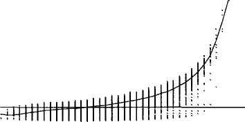
The panels in Figure la plot, for the universe of seven-party systems where the largest party is dominant, the relationship between party size and the attractiveness (EWR) for the largest three parties. The left-hand column of panels shows the impact of the size of the top three parties on the attractiveness of the largest party in minority legislatures. The center and right columns do the same for the attractiveness of the second party and third-largest parties.¹⁶ The top row of panels shows the impact of the size of the largest party on the attractiveness of each of the first three parties. The middle row shows the impact

¹⁶The relationships we have plotted for the seven-party case is perfectly typical of the four- through ten-party systems. The graphs for the other и-party minority legislatures, for those with and without a dominant party, may be viewed at our web site at http://www.tcd.ie/PoliticaLScience/.

Figure 1a Expectation-to-Weight Ratios by Proportion of Seats, First, Second, and Third Parties, When the Largest Party Is Dominant, 7-Party Legislature

2 ' .5 -

7 Paroes, Dominant Party

0 -

₁

_!!•

_i_{•
■ '}

% Seats ot Largest Party

2 -

7 Parties, Dom III

nant

.5 "

₁

_м_I^:_■

-5 -0 -

2 " 1.5 -i

7 Parties, Dominant Party

lii

1 -.5-0-

_IP

_■

% Seats of Largest Party

2 -

1 -5-

/Part

as, Do >

ninant

;

irt

• i

₁

_III!:::

0 -

7 Parties, Dominant Party

7Parties, Dominant Party

% Seats of Largest Party

hi П

K> Seats of 2nd Largest Party

% Seats of 2nd Largest Party

% Seats ot 2nd Largest Party

7 Parties, Dominant Party

; |

,—•—-l^_

: i

■ i

%Seals of Party 3

a is-


_M	-	-	-	•**	I !
24

% Seats of Party 3

% Seats ot Party 3

Figure 1b Expectation-to-Weight Ratios by Proportion of Seats, First, Second, and Third Parties, When the Largest Party Is Not Dominant, 7-Party Legislature

7 Parlies, No Dominant Party

_S_"^A

2 " 1.5 -

7 Parties, No Dominant Party

1 -

.5-0 -

] 1! i:!' H I i| i ii 11jj

7 Parties, No Dominant Party

% Seats оГ Largest Party

% Seats of Largest Party

7 Parties, No Dominant Party

7 Parties, No Dorrinant Party

_i			_Ii
			...«tnhimt^

| '^И

% Seats of 2nd Largest Party

% Seats ol 2nd Largest Party

% Seats of 2nd Largest Party

7 Parties, No Dominant Party

7 Parlies, No Dominant Party

7 Parties, No Dominant Party

i'iij-
						_Illllll"¹_'

% Seats of Party 3

% Seats or Party 3

I 1 I liT

%Seats of Party 3

THE EVOLUTION OF PARTY SYSTEMS BETWEEN ELECTIONS

227

of the size of the second-largest party, and the bottom row shows the impact of the third-largest party. Figure lb provides identical information for the universe of cases when the largest party is not dominant.¹⁷

The clouds of points in these graphs are scatterplots (with very large numbers of points) showing areas where there is at least one observation in the metadataset. Blank areas show where there is no observation. The curved lines running through these clouds of points show median splines linking the median EWR for all parties with a given share of the seats. The horizontal straight line in each plot shows the "proportional expectation" (EWR =1) values for each party size. Parties above this line have EWRs of greater than unity and must therefore be attractive to members of some other party. Parties below the line have EWRs of less than unity and must have members who are attracted to some other party. These scatterplot matrices and median splines convey a wide range of information about the implications of our model.

The top left panel of Table la, showing how the EWR of a dominant largest party is affected by its own size, shows that the median spline is always above the proportional expectation line for dominant largest parties, rising steadily higher as party size increases. The cloud of points dips below the EWR = 1 line, showing that it is possible to find dominant largest parties with EWRs of less than unity (and which are therefore relatively unattractive). This shows that we should resist the temptation to assume that, simply because a party is dominant, it will necessarily be attractive to defectors from other parties. The median spline shows quite clearly, however, in line with our analytical expectations that the typical dominant largest party has EWRs of greater than unity and is indeed attractive to putative defectors from at least one other party.

The cloud of points in the top left panel of Table lb shows that, when nondominant largest parties control more than one-third of all seats, they always have EWRs of less than unity, being less attractive to members of other parties and having members who will be attracted to other parties. This is in line with our theoretical expectations. Going beyond our analytical results, we see from the median spline that even below this threshold the EWR of the typical nondominant largest parties is barely greater than unity. In substantive terms this shows that the attractiveness of the largest party to defectors typically arises when it is dominant, not coming from size in itself nor even from being the largest party per se.

¹⁷ These plots exclude configurations in which there were ties in size among the top three parties, since in these cases the meaning of the terms "largest," "second-largest," etc., are ambiguous. Such cases are rare in real legislatures.

We see from the clouds of points and median splines in the center panels of Figure la and lb that the second-largest party does, in line with the analytically derived upper bound, hit a wall at one-third of the seats, never having EWRs of greater than unity and becoming increasingly less attractive to putative defectors when it wins more seats than this. Going beyond these analytical bounds, we see that the clouds of points do move above the EWR = 1 line at party sizes below one-third of the total in each universe of cases, so that it is certainly possible to find potentially attractive second-largest parties. However the median splines in each universe show that the typical second-largest party almost always has an EWR of less than unity whatever its size, particularly when the largest party is dominant. This implies that, in stark contrast to the position of the largest party, the second-largest party is typically much less attractive to putative defectors.

The conjecture that there will be intense competition between the first- and second-largest parties is convincingly supported by comparing the center-left and top-center panels in both Figure la and Figure lb. These show how, with or without a dominant party, the attractiveness of the largest party varies inversely with the size of the second-largest and how the attractiveness of the second-largest party varies inversely with the size of the largest. Even a typical dominant party declines relentlessly in attractiveness as the size of the second-largest party increases. (This is in stark contrast to the impact of the third-largest party on the attractiveness of the largest— see the bottom-left panel of each figure.) Similarly, the attractiveness of the second-largest party declines relentlessly as the size of the largest party increases. This pair of inverse relationships is one of the clearest features of all scatterplot matrices we have generated and provides a logic for intense competition between the two largest parties in the interelectoral evolution of office-seeking party systems.

We see from the bottom right panel in Figure la and lb that, in line with our analytical expectations, third-largest parties are typically much more likely than second-largest parties to have high EWRs and hence to be attractive to putative defectors from other parties. They can achieve very high EWRs—far higher than those for either first-or-second-largest parties indeed—especially when they control relatively few seats.

Similar expectation-to-weight plots for all other party ranks in the universe of seven-party systems show that the smaller parties (those not among the largest three) are more or less equally likely to have EWRs of greater or less than unity. There is no systematic attractiveness bias for or against the lower-ranked parties, in contrast to the bias

228

MICHAEL LAYER AND KENNETH BENOIT

Table 2 Proportions of Relevant Cases for Which One Party in the System Is Attractive to Members of Another

			Proportion of NEDs where legislators from party below find column 1
	Potential	Largest Party			party attractive
	Attractor	Dominant?	PI	P2	P3	P4	P5	P6	P7
я = 5
	PI	Dominant	-	.97	.63	.61	.61	-	-
		Not	-	.00	.19	.83	.71	-	-
	Р2	Dominant	.03	-	.02	.25	.45	-	-
		Not	1.00	-	.22	.87	.76	-	-
	РЗ	Dominant	.37	.98	-	.36	.57	-	-
		Not	.81	.76	-	.67	.67	-	-
	Р4	Dominant	.39	.75	.55	-	.39	-	-
		Not	.17	.13	.23	-	.00	-	-
	Р5	Dominant	.39	.55	.42	.50	-	-	-
		Not	.29	.24	.32	.28	-	-	-
п = 6
	Р1	Dominant	-	.95	.69	.75	.73	.66	-
		Not	-	.20	.37	.79	.60	.78	-
	Р2	Dominant	.05	-	.12	.36	.45	.46	-
		Not	.80	-	.30	.74	.57	.75	-
	РЗ	Dominant	.31	.88	-	.44	.58	.58	-
		Not	.63	.70	-	.59	.54	.77	-
	Р4	Dominant	.25	.64	.44	-	.36	.49	-
		Not	.21	.26	.25	-	.05	.34	-
	Р5	Dominant	.27	.54	.40	.48	-	.30	-
		Not	.40	.43	.43	.46	-	.36	-
	Р6	Dominant	.34	.54	.42	.49	.44	-	-
		Not	.22	.25	.23	.29	.20	-	-
п = 1	Р1	Dominant		.95	.74	.84	.81	.77	.74
		Not	-	.46	.59	.82	.63	.79	.74
	Р2	Dominant	.05	-	.19	.41	.47	.47	.50
		Not	.54	-	.45	.73	.53	.72	.71
	РЗ	Dominant	.26	.81	-	.50	.61	.61	.63
		Not	.41	.55	-	.54	.48	.70	.67
	Р4	Dominant	.16	.58	.36	-	.37	.47	.52
		Not	.18	.27	.25	-	.15	.43	.47
	Р5	Dominant	.19	.53	.37	.44	-	.32	.46
		Not	.37	.47	.48	.52	-	.46	.53
	Р6	Dominant	.23	.53	.39	.49	.41	-	.32
		Not	.21	.28	.30	.38	.23	-	.30
	Р7	Dominant	.26	.50	.37	.47	.46	.36	-
		Not	.26	.29	.33	.37	.29	.34	-

Note: All data is for minority legislatures only and excludes any ties between PI, P2, and P3.

in favor of the largest party, against the second largest, and in favor of the third.¹⁸

¹⁸ These plots, and results for party systems of other sizes, can be viewed on our website http://www.tcd.ie/Political.Science/ fissionfusion/.

The general patterns in the scatterplot matrices are confirmed systematically in Table 2. This shows the relative frequency, in the different party system universes, with which a party at one position in the ranking is attractive to legislators from a party at another position.

THE EVOLUTION OF PARTY SYSTEMS BETWEEN ELECTIONS

229

As a representation of the general pattern, we display the attractiveness matrixes for the five, six, and seven-party universes, broken down by whether there was a dominant party or not.

First, reading along the top two rows for each party universe, we see that dominant party status makes the largest party much more attractive to legislators in the second- and third-largest parties. Thus, in the universe of five-party systems, dominant largest parties are attractive to legislators from 97% of all second-largest parties, while nondominant largest parties are never attractive to legislators of second-largest parties. Also in the universe of five-party systems, dominant largest parties are attractive to legislators from 63% of all third-largest parties, while nondominant largest parties are attractive to legislators from only 19% of third-largest parties. The magnitude of this effect declines as the size of the party universe increases.

Second, continuing along the top two rows, dominant party status has no systematic effect on the attractiveness of the largest party to legislators from the smaller parties. Certainly in terms of the likelihood of finding their legislators attracted to the largest party, the second- and third-largest parties seem to be in a quite different position from that of the smaller parties.

A third remarkable trend concerns the attractiveness of the second-largest party to the largest. When the largest party is dominant, the second-largest party is almost never attractive to legislators in the largest party. However, when largest party is not dominant, its legislators are more often than not attracted to the second largest. Thus, looking at the six-party universe, legislators from a dominant largest party are attracted to the second-largest party in only 5% of cases. But legislators from a nondominant largest party are attracted to the second-largest party in 80% of cases. Being a nondominant largest party typically offers no protection against the temptation of your members to defect to the second largest in the interelectoral evolution of an office-seeking party system.

Overall, these results underline two substantively interesting patterns that reappear throughout our analysis. The first is the intense competition between the first- and second-largest parties in the interelectoral evolution of multiparty systems. The second is way in which the existence or not of a dominant party transforms the entire system. If largest party is dominant, then the second-largest party is in a very weak position. It is unattractive to other parties, and its legislators are much more likely to be attracted to other parties, especially the largest party. If the largest party is not dominant, then the position of the second-largest party is completely different. It is much more likely to attract defections from other parties, in-

cluding the largest party, and much more likely to hold on to its own members. This strongly suggests that the existence of a dominant party is a very important feature conditioning the interelectoral evolution of any office-seeking party system.

Attractiveness and Dominance

All of this means that it is important to be able to characterize systems in which there is a dominant party. We know analytically that the largest party must control more than 25% of the seats to be dominant. Figure 2 confirms this, showing the relationship between the size of the largest party and the proportion of largest parties that are dominant in the various party-system universes. The effect of the 25% threshold is strongly revealed. Equally striking and going well beyond previous results is that, in the systems with six or more parties, the largest party typically becomes dominant as soon as it passes the 25% threshold. Substantively, this implies in larger party systems that a largest party with over 25% of the seats is likely to prove a pole of attraction in interelectoral party-system evolution. If the largest party has less than 25% of the seats, it is not likely to be a pole of attraction.

Size, Attractiveness, and Willingness

As well as characterizing attractiveness, our computational results, and in particular the slope of the median spline in the graphs plotting the EWR of a party against its own size (the top-left to bottom-right diagonal panels in Figure la and lb), allow us to go beyond our analytical conclusions about willingness to accept defections. These splines summarize the extent to which EWR increases as size increases. When the largest party is dominant (Figure la), the median spline for the largest party takes on a positive slope above a certain threshold. Above this threshold, the addition of a single seat to the total of the largest party more often than not produces a dispropor-tional increase in the median expectation for that party.¹⁹This must be the result of a number of largest parties increasing expectations as a result of accepting defectors. The positive slope of the median spline thus identifies a systematic increase, with increasing size, in the numbers of largest parties whose members are willing to accept defectors. The position of the median spline above the EWR — 1 line, as we have already seen, shows when

¹⁹If the acceptance of an additional legislator either had no effect on the expectations of largest parties, or increased expectations only in as a many parties as it decreased them, then the median spline wold not rise in this way as party size is increased by one.

Figure 2 The Incidence of Dominant Parties, by Size of Largest Party, in the Universes of 4-10 Party Legislatures (Minority Legislatures Only, with pi = pi, p2 = p3, pi = p2 = p3 Ties Excluded)

100 Seat Legislature, 4 Parties

100 Seat Legislature, 5 Parties

100 Seat Legislature, 6 Parties

10 15 20 25 30 35 40 45 50