

ZAMBAK_IT_Excel2010
.pdf8.6 Tracking
Microsoft Excel can maintain and display information about how a worksheet has been changed. Change Tracking logs details about workbook changes each time you save a workbook. You can use this history to understand what changes were made, and accept or reject changes. This capability is particularly useful when several users edit a workbook. It is also useful when you submit a workbook to reviewers for comments, and then want to merge input into one copy, deciding which changes and comments to keep.
8.6.1 How to Use Change Tracking
To activate Tracking changes, firstly, your workbook cannot contain any table (table which is defined by Office as a Table). If your workbook is OK with this, save it first and click the Highlight changes button from Review ChangesTrack Changes.
Figure 8.23a: Highlight Changes
Figure 8.23b: Highlight Changes dialog box
It’ll open the Highlight Changes dialog box. Select the ‘Track changes while editing’ check box. This will activate the When, Who and Where boxes. Select the necessary information for these boxes. For the address in the Where box, click in the box first, then, without closing the dialog box, go and select the range that you want to keep tracking. Excel will automatically write the selected range address there. After you finish all, click OK.
This will start sharing your workbook and in your taskbar, your filename will include the [Shared] word in brackets.
Extra Options |
141 |
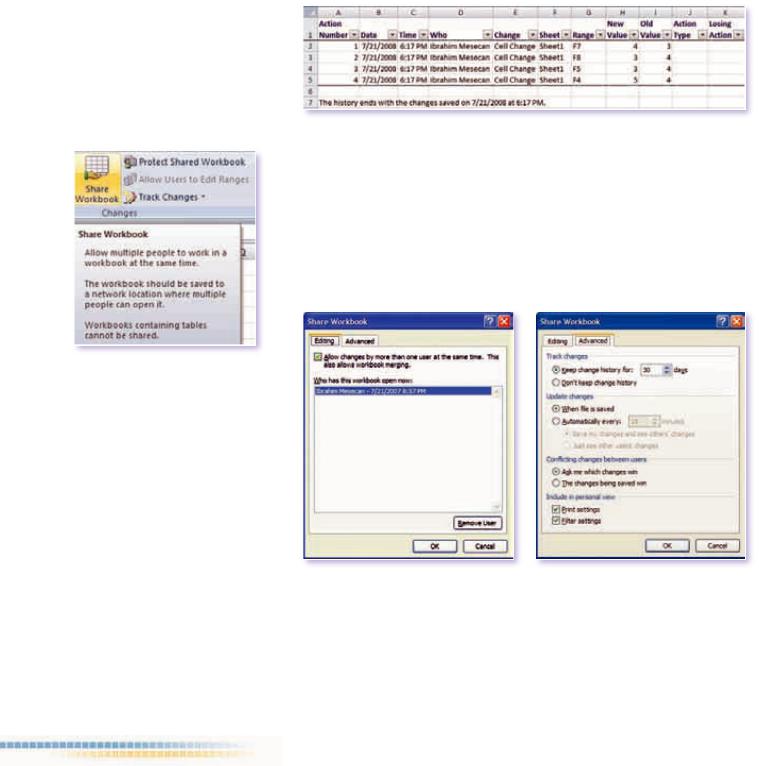
List changes on a new sheet: Displays the changes on a separate history worksheet that you use to filter the information to find the changes you want. This check box is available only after the workbook has been saved as a shared workbook.
Figure 8.24: List changes on a new sheet
8.6.2 Sharing a Workbook
Sharing a workbook is another way to collaborate data. You can share a workbook to allow changes by more than one user at the same time.
You share a workbook using the Share Workbook button from the Review Changes tab. This also allows workbook merging. You can remove any users you do not want to use the shared workbook.
Figure 8.25: Sharing a workbook
Figure 8.26: Sharing a workbook
You can adjust more options in the Advanced tab. Track Changes: Specifies whether to maintain the change history when you share the workbook. Update Changes: Specifies how long you want to see changes from other users. Conflicting changes between users: Specifies how you want to review conflicting changes when you save the shared workbook.
142 |
Microsoft Excel |

Include in personal view: specifies personal printing and filtering options for the shared workbook. If you select one or both of the options below, your choices are independently saved with your copy of the shared workbook. After you share the workbook you can check who changed the document.
8.6.3 Display changes
Using Accept or Reject Changes from Review Changes Track Changes, you can accept or reject any change in the workbook. When you click on this button Excel will first ask for saving the changes. After that, it’ll open the “Accept or Reject Changes” dialog box.
Figure 8.27: Accept or reject changes
It’ll show each change in the dialog box and on the sheet, and ask you to Accept or Reject.
Untracked changes
Not all the changes are tracked. So be careful when you make the following changes.
Change sheet names
Insert or delete worksheets
Format cells or data
Hide or unhide rows or columns
Add or change comments
Cells that change because a formula calculates a new value
Unsaved changes
Extra Options |
143 |

Figure 8.28:
Office Menu Excel Options
8.7Options Window
You can open the Options window from the Excel Options button in the Office Menu. The Options window is like the headquarters of Microsoft Excel. It provides flexibility according to user demands, which is very important in user interface and user friendly environments. The options window contains hundreds of different options for the user interface.
The good side of this new Excel Options is that, different than the older versions, you can reach all options from a single dialog box. In this Options window, there are 10 pages including: General, Formulas, Save, Advanced, etc.
8.7.1 General Tab
The General Tab contains mostly visual options. You can change color scheme, show/hide the Mini toolbar and activate or deactivate Enable Live Preview. With the help of Live Preview, when pointing to various formatting choices, you can instantly see how those choices would appear on selected text and objects. You also have different Screen tip options.
There are also default workbook properties when creating a new one. We have font, default number of sheets for a new workbook, default view style, etc. options for new workbooks.
Figure 8.29: Office Menu Excel Options
144 |
Microsoft Excel |

From this tab, you can
Enable Live Preview
Change color scheme,
Change Screen tip style
Define the number of worksheets,
Change default fonts,
8.7.2 Formula options
This tab includes options related to the Formula calculation, performance, and error handling options.
Calculation options
Workbook Calculation specifies how you want Microsoft Office Excel to calculate workbooks: Automatic, Automatic except for data tables, Manual, etc.
Enable iterative calculation: When this option is selected, it allows iterative formulas (also known as circular references) to be calculated. Unless you specify otherwise, Excel stops after 100 iterations or when all values change by less than 0.001.
Figure 8.30: Formula options
Extra Options |
145 |

Using your programming capabilities, you can also write your own function that converts R1C1 into A1 reference style. (This can be a good case study).
Working with formulas
R1C1 reference style: You can switch between A1 and R1C1 reference styles. In the A1 reference style rows are referenced by numbers and columns are referenced by letters. But, the R1C1 style refers to both, rows and columns, directly by numbers in your references. The R1C1 reference style might be easier to use when you have complex macros and formulas.
Formula AutoComplete: providing tools help you to write your formulas easily.
Use table names in formulas: When you use formulas that reference a table, this option makes it easier to work.
Use GetPivotTable functions for PivotTable references: Determines the type of cell reference that is created for a PivotTable cell
Error Checking
Enable background error checking: Select to have Excel check cells for errors when idle. If a cell is found to have an error, the cell is flagged with an indicator in the upper left corner of the cell.
8.7.3 Proofing Options
Proofing options includes Language tools. You should be familiar with the AutoCorrect Options from MS. WORD. Using AutoCorrect you can correct your misspelled words automatically. Or, you can create new shortcut words for your company initials, etc. e.g. you can select to replace your initials ‘im’ with your name ‘Ibrahim Mesecan’.
|
|
|
Figure 8.31a: Proofing Options |
|
Figure 8.31b: AutoCorrect Options |
146 |
Microsoft Excel |

You can add, create new or remove your custom dictionaries. Or, you can add edit them. There are also options for: checking for repeated words, ignoring words in UPPERCASE, etc.
8.7.4 Save Options
As it’s clear from the name, this tab contains the options for saving. You can change
Default save format.
Saving time for the Auto Recovery file
Default file location
Offline editing options for document management server files
AutoRecover exceptions
Preserve visual appearance of the workbook for the
Figure 8.32: Save options
8.7.5 Advanced Options
Probably, the most commonly used tab. It contains many different options in different categories:
Editing options contains the options when editing a worksheet, like:
After pressing Enter, move selection down;
Enabiling fill handle and cell drag-and- drop;
Allow editing directly in cells;
Enable AutoComplete for cell values;
Use system separators, is nice if you don’t want to change your system setting but you want to change how
Excel handles numbers with floating
Figure 8.33: Advanced options
point. Etc.
Extra Options |
147 |

Cut, Copy, and Paste options
Display contains the options like:
Show this number of Recent Documents;
Show function ScreenTips;
Options for cells with comments; etc.
Display options for this workbook/worksheet
General Options:
Enable multi-threaded calculation: This option enables fast calculation by using all of the processors on your computer or by using the number of processors that you type manually;
When calculating this workbook
Update links to other documents;
Set precision as displayed: Permanently changes stored values in cells from full precision (15 digits) to whatever format is displayed, including decimal places. Be careful that, this can cause your data to lose precision. Etc.
Lotus Compatibility
|
|
|
Custom Lists |
|
|
|
|
Using this option, other than regular numerical |
|
|
|
|
ones, you can create your own lists. You |
|
|
|
|
commonly use the day or month lists. After you |
|
|
|
|
define something as a list, you can |
|
|
|
|
automatically fill a series of days, months, |
|
|
|
|
etc… by using Fill Series option. |
|
|
|
|
First, write your series in cells in a worksheet. |
|
4 |
|
|
Then, open the Custom Lists from Options |
|
|
|
dialog box and |
2 |
|
|
|
|
to select your Custom list range. After you |
|
|
|
|
select the range of the list, press ENTER. This |
|
|
|
|
will take the address of the list to the Import |
|
1 |
2 |
3 |
from cells |
1 . After that, click the Import |
|
|
|
button 3 , |
will be added into Custom |
Lists 4
Figure 8.34a: Creating Custom Lists
148 |
Microsoft Excel |
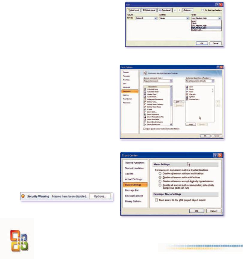
In order to sort a list according to this custom lists:
First Add your list into Custom lists
Then select your range, and click the Sort & Filter button from Home Editing to display the Sort dialog box
Select Column and Sort On combo boxes properly
Then, select Custom Lists from the Order Combo box
It will show you the Custom Lists Dialog box, Select your custom list and press OK.
8.7.6 Customize Ribbon and QAT
Ribbon doesn’t include all the commands that you can use in Excel. By using Customize you can change your Quick Access Toolbar, so that, you can add new commands that are not available in the ribbon or you commonly use but not easy to access from the ribbon.
You can also prepare your own tab in the Office 2010.
8.7.7 Trust Center
Because macros could be very dangerous, you needed to be very careful when opening Excel documents in earlier Excel versions. But now, developers of Excel made a lot of improvements. The most essential change is the Macro containing files’ extensions. If an Excel document contains macros, it is saved with .xlsm extension. The good side is that, in a way, if the extension is changed to .xlsx Excel will not open it and warn that this is not a recognized format.
In general, Trust Center is the essential window for security. By default, developers setup it quite secure. You just need to be careful when you see a warning message over Formula bar:
If you click the Options button, it’ll show the MS. Security Options dialog box. If you trust the sender of the file you can enable the macro. If you are not sure what to do, you should better protect yourself.
Figure 8.34b: Using Custom Lists
Figure 8.35: Customizing QAT
Figure 8.36: Trust Center Options
Extra Options |
149 |

Questions
1.………… validation criteria allow the user to enter anything in the cell.
6.When you ‘Highlight Changes’, which of the changes below is tracked?
a. Decimal |
b. Any value |
a. Change sheet names |
c. List |
d. Custom |
b. Insert or delete worksheets |
|
|
c. Add or change comments |
|
|
d. Changing the formula of a cell |
2.The ………… validation criteria allows you to enter your birthday to the cell.?
a. Decimal |
b. Date |
c. Time |
d. Text Length |
3.Which is the Excel Options button located?
a.In Home tab
b.In Office menu
c.In View tab
d.In QAT
According to the default Excel settings, choose the right one.
7. Gridlines are hidden.
TRUE FALSE NOT DEFINED
8.The resulting value of any formula can be seen in cells.
TRUE FALSE NOT DEFINED
4. You can change the comment shape.
TRUE |
FALSE |
5.If the manual option is selected from the calculation tab on the Options window, which key is used to recalculate the formulas?
a. F5 |
b. F8 |
c. F7 |
d. F9 |
9.The Horizontal scroll bar cannot be seen on this worksheet.
TRUE FALSE NOT DEFINED
10.This ‘View settings’ does not effect other sheets in the same workbook.
TRUE FALSE NOT DEFINED
11. Function screentips are visible.
TRUE FALSE NOT DEFINED
150 |
Microsoft Excel |