

ZAMBAK_IT_Excel2010
.pdf14.There is an international Informatics Olympiad in your country. They prepared a table after the exam. For some statistical purposes, they want to get some information from the table. Write the necessary formulas
In cell F18 to show the number of students who did not participate on the first day;
to show each student's total points in the column F
in cell F20, to show the number of students from the given country, in the cell B20.
A |
B |
C |
D |
E |
F |
1The Results of the Informatics Olympiad
2 |
Rank |
Name and |
Country |
1st |
|
2nd |
TOTAL |
|
|
Surname |
|
Day |
|
Day |
|
3 |
4 |
Slena Bainum |
England |
140 |
|
120 |
260 |
4 |
8 |
Geoff Bowers |
France |
150 |
|
80 |
230 |
5 |
3 |
Rab Brooks |
England |
120 |
|
150 |
270 |
6 |
9 |
Raymond Camden |
Switzerland |
|
|
210 |
210 |
7 |
6 |
Adam Churvis |
Germany |
150 |
|
100 |
250 |
8 |
12 |
Michael Dinowitz |
USA |
|
|
180 |
180 |
9 |
1 |
Shlomy Gants |
Germany |
180 |
|
155 |
335 |
10 |
14 |
Paul Hastings |
USA |
|
|
100 |
100 |
11 |
11 |
Alexandra Kim |
Korea |
52 |
|
150 |
202 |
12 |
9 |
Viktoria Shay |
Korea |
|
|
210 |
210 |
13 |
2 |
Olga Nam |
Korea |
85 |
|
200 |
285 |
14 |
7 |
Brendan Hara |
Spain |
|
|
240 |
240 |
15 |
13 |
Jeremy Peterson |
England |
50 |
|
120 |
170 |
16 |
14 |
Todd Rafferty |
Switzerland |
|
|
100 |
100 |
17 |
4 |
Kevin Schmidt |
England |
80 |
|
180 |
260 |
18 |
How |
many contestants are |
absent on the |
1st Day? |
6 |
||
19 |
How many contestants are there on the 2nd Day? |
15 |
|||||
20 |
Country |
Korea |
Number of the |
|
3 |
||
Contestants |
|
||||||
|
|
|
|
|
|||
|
|
|
|
|
|
|
|
15.A cellular base-station is located at the coordinates (x1, y1) and it has a transmit range of “r” . A person using a mobile phone is located at the coordinates (x2,y2).
Write a function that gets (x1,y1), (x2,y2) coordinates and the radius of the transmitter and then decides if the mobile phone is in use or not . If the phone works, the message will be “The phone is working in this location”, otherwise, “The phone is out of range”. Note: Use the If function.
|
A |
B |
C |
D |
1 |
x1: |
100 |
x2: |
60 |
2 |
y1: |
100 |
y2: |
40 |
3 |
r* |
50 |
The phone is out of rance |
|
16. In the following sheet, the actual username and password are stored in C1 and |
|
A |
B |
C2. If the correct user name and password are entered in B1 and B2, the |
1 |
User Name: |
admin |
message in A3 will be “Welcome to the Matrix”; otherwise, “Incorrect user name |
2 |
Password: |
x-man |
or password”. |
3 |
Welcome to |
The Matrix |
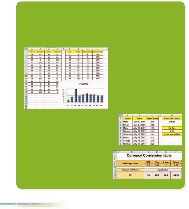
17.Prepare the frequency chart of the exam results of 4 Classes. You can use the CountIfs function to count the number of cells between low and high values.
18.In a sheet you keep the Extra work hours of your staff. Write a function in E5 that gives the total hours for the person written in E2 cell.
19.Prepare the following figure using the absolute reference formula in the cells C12:F12.
Note: Multiply the exchange rates in C9:F9 with A12 to produce the results.

DATA PROCESSING
In most cases, the vision and prestige of your company is much more important than the money you spend on technology. If you don’t spend enough money and time for data processing, or for technology, it will most probably cost more. The small mistakes that you make can damage your company image a lot. Especially, when working with huge lists and lots of numbers, fast and accurate results need proper investments.
6.1 Preparing Lists
Microsoft Excel is perfect when you have huge lists with lots of numbers and calculations. It has many fast and easy to use tools to analyze and process data. Sorting and Filtering are two examples of this.
A simple example that shows the advantage of sorting is the telephone guide. In telephone guides for many cities, you have hundreds of thousands of names. Can you imagine what would happen if the names in these guides were not in order? You would need to search, sometimes for many days, to find a single name. But since the names are in order you easily find a name in minutes.
For a good analysis of data, firstly, you need to prepare well organized data lists. This is called a Database. There are some important rules when preparing lists.
1.Before you start any other operation, perhaps the most important part is to think carefully and decide the titles of the list. After you start collecting data, it can be very difficult to add another field to your list.
2.The same type of information must be entered to each column. For example; for a travel agency's records, you may assign name, date of reservation, hotel, suite type, payment type, and total price, etc. as column titles.
3.It is better to prepare single purpose clear titles. Try avoiding mixed columns. For example, if you store hotel name and suit type in the same column, you might have difficulty later.
4.Try to avoid blank rows and columns.
6.2Sorting
Sorting means putting or arranging items in order, according to some criteria. Sorting is commonly used with lists. In many conditions, you prepare lists and put them in order.
6.2.1 Using Fast Sort
When you have a simple sort (sorting according to one field), first, you select the range using your mouse (or keyboard). Then, using your Tab and Enter keys, activate the column according to which you want your list to be sorted.
104 |
Microsoft Excel |
Finally, Select “Sort A to Z” (or “Sort Z to A”) button from Home Editing. You can also right click on the selected range and select an option from the Sort list. But, for a better and more accurate result, it is suggested to use the Custom Sort dialog box.
Example 6.1:
Put the list below in the Date order.
Class |
Name |
Surname |
Date |
Lesson |
Hours |
Motivated |
|
|
|
|
|
|
|
11A |
David |
Shadovitz |
2/19/2007 |
Math’s |
2 |
TRUE |
11A |
David |
Shadovitz |
3/2/2007 |
Chemistry |
2 |
FALSE |
11A |
David |
Shadovitz |
3/2/2007 |
Informatics |
1 |
TRUE |
11A |
David |
Watson |
2/26/2007 |
Physics |
2 |
TRUE |
11A |
Pablo |
Varando |
2/19/2007 |
Chemistry |
2 |
TRUE |
11A |
Todd |
Rafferty |
2/22/2007 |
Physics |
2 |
FALSE |
|
|
|
|
|
|
|
Figure 6.2: Attendance list
To do this:
Firstly select the list including the header row
Using your Tab and Enter keys activate the Date title
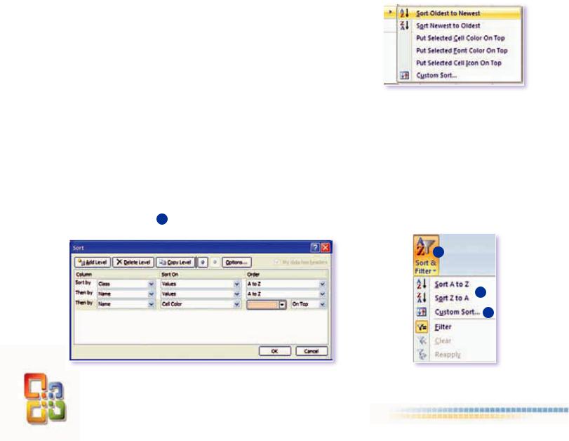
Then Right click on the list and select Sort Sort Oldest to Newest (Figure 6.1) from the popup menu
6.2.2 Custom Sort
Microsoft Excel provides an easy feature to put the items in order; the Sort dialog box.
Click on a cell in the range that you want to sort. Excel will automatically determine the extent of the list. If you don’t want to include the entire list, and you want to sort only a part of it; or, if somehow Excel cannot determine the exact range; Select the range of cells yourself
Click the Custom Sort 3 button from Home Editing Sort & Filter to display the Sort dialog box, Figure 6.4.
Figure 6.4: The Sort dialog box
Figure 6.1: Faster Sort
1
2
3
Figure 6.3: Sort & Filter commands
Data Processing |
105 |

Click on the Sort by down arrow to select the column you want (Class).
From the “Sort On” combo box (the second one), select either to sort according to cell values, or cell color etc. (Values)
From the Order combo box (the third one), select sorting order (A to Z)
If you want to use more than one criterion, you can use the Add Level button for more criteria.
Click “My Data has headers” to exclude/include the first row from the sort.
If you want to remove a sorting level, first activate it and use the Delete Level button
Using the Options button, for the column, selected in the Sort by box, you can also specify a case-sensitive sort and sort either from top to bottom or from left to right. In Excel 2003, we could use only 3 levels of sorting criteria. Now, it supports 64 levels of criteria and more options in every criterion.
Example 6.2:
Data is sorted according to the Date field. Put the list below in the Name order.
Class |
Name |
Surname |
Date |
Lesson |
Hours |
Motivated |
|
|
|
|
|
|
|
|
|
11A |
David |
Shadovitz |
2/19/2007 |
Math’s |
2 |
|
TRUE |
|
|
|
|
|
|
|
|
11A |
Pablo |
Varando |
2/26/2007 |
Chemistry |
2 |
|
TRUE |
|
|
|
|
|
|
|
|
11A |
Todd |
Rafferty |
2/26/2007 |
Physics |
2 |
|
FALSE |
|
|
|
|
|
|
|
|
11A |
David |
Watson |
2/26/2007 |
Physics |
2 |
|
TRUE |
|
|
|
|
|
|
|
|
11A |
David |
Shadovitz |
3/2/2007 |
Chemistry |
2 |
|
FALSE |
|
|
|
|
|
|
|
|
11A |
David |
Shadovitz |
3/2/2007 |
Informatics |
1 |
|
TRUE |
|
|
|
|
|
|
|
|
Firstly, if you sort it using ‘Quick Sort option’ by Name, you’ll get: |
|
||||||
|
|
|
|
|
|
|
|
Class |
Name |
Surname |
Date |
Lesson |
Hours |
Motivated |
|
|
|
|
|
|
|
|
|
11A |
David |
Shadovitz |
2/19/2007 |
Math’s |
2 |
|
TRUE |
|
|
|
|
|
|
|
|
11A |
David |
Watson |
2/26/2007 |
Chemistry |
2 |
|
TRUE |
|
|
|
|
|
|
|
|
11A |
David |
Shadovitz |
3/2/2007 |
Physics |
2 |
|
FALSE |
|
|
|
|
|
|
|
|
11A |
David |
Shadovitz |
3/2/2007 |
Physics |
1 |
|
TRUE |
|
|
|
|
|
|
|
|
11A |
Pablo |
Varando |
2/19/2007 |
Chemistry |
2 |
|
TRUE |
|
|
|
|
|
|
|
|
11A |
Todd |
Rafferty |
2/22/2007 |
Physics |
2 |
|
FALSE |
|
|
|
|
|
|
|
|
Figure 6.5: Before and after sorting
106 |
Microsoft Excel |
But as you see from the list above, just sorting according to one field will not resolve your problems in may cases. Here, David Watson’s absence is listed in the middle of the absences from David Shadovitz. So, it’s not the desired result. We should sort the list using two criteria, for this purpose: First by Name; then by Surname.
To do this:
Firstly select the list including the header row
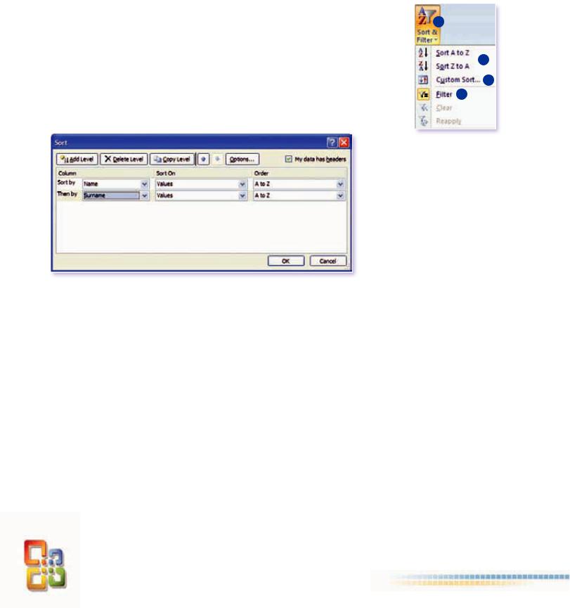
Then click “Custom Sort” from Home Tab Editing Sort&Filter (Figure 6.6)
It’ll open the Sort dialog box (Figure 6.7)
Figure 6.7: Sort Dialog Box
Select Name from the Column combo box then
Click the Add Level button this will open new level
Select the Surname field from the second column list
Press OK.
Class |
Name |
Surname |
Date |
Lesson |
Hours |
Motivated |
|
|
|
|
|
|
|
11A |
David |
Shadovitz |
2/19/2007 |
Math’s |
2 |
TRUE |
|
|
|
|
|
|
|
11A |
David |
Shadovitz |
3/2/2007 |
Chemistry |
2 |
FALSE |
|
|
|
|
|
|
|
11A |
David |
Shadovitz |
3/2/2007 |
Informatics |
1 |
TRUE |
|
|
|
|
|
|
|
11A |
David |
Watson |
2/26/2007 |
Physics |
2 |
TRUE |
|
|
|
|
|
|
|
11A |
Pablo |
Varando |
2/19/2007 |
Chemistry |
2 |
TRUE |
|
|
|
|
|
|
|
11A |
Todd |
Rafferty |
2/22/2007 |
Physics |
2 |
FALSE |
|
|
|
|
|
|
|
Figure 6.8: The sorted list: by Name and then by Surname
1
2
3
4
Figure |
Custom sort |
Data Processing |
107 |
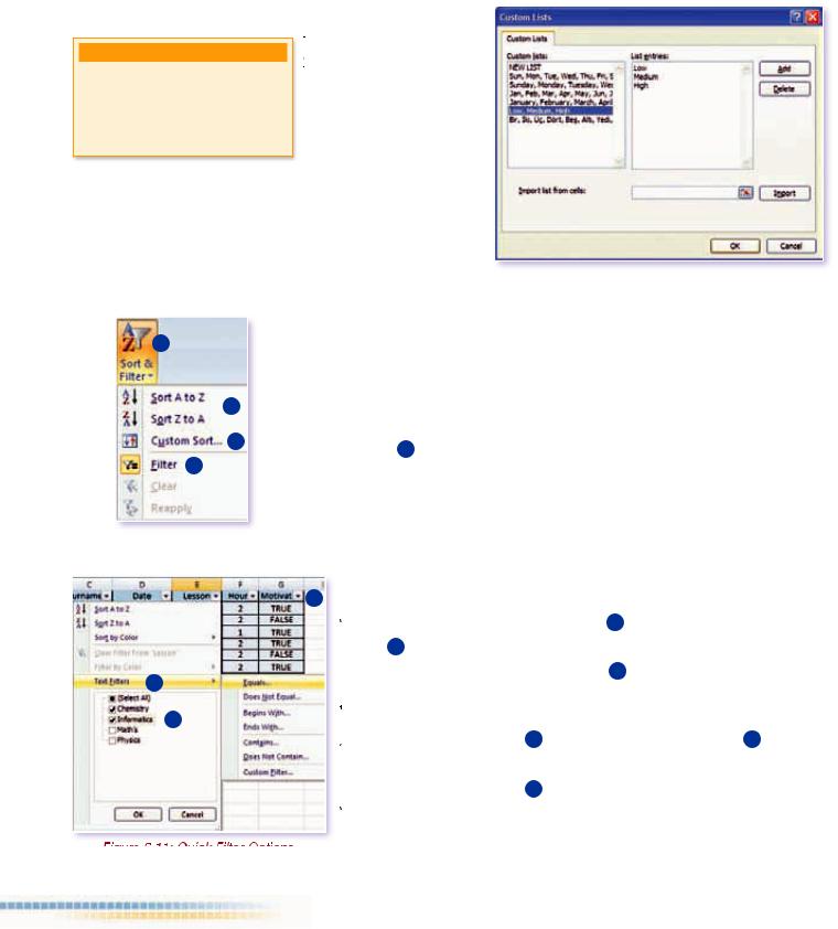
6.2.3 Custom Lists
You can show Custom Lists dialog box from
Excel Options Advanced Edit
Custom Lists ...
The Custom List option lets you specify a custom sort  order; such as Low, Medium, High; or Jan, Feb, Mar, so
  forth. You can write your list
  order in the List Entries
  column, and click on the Add button to add this to the Custom lists. Your Custom List is ready to be used in sorting orders now. Custom Lists is explained in Chapter 8.7.5.
Figure 6.9: Custom Lists dialog box
1
6.3 Filtering
Filtering is a quick and easy way to find and work with a subset in a data list.
2A filtered list displays only the rows that meet the criteria you specify for a list.
|
Microsoft |
|
provides two commands for filtering lists: |
|
3 |
|
4 |
simple criteria |
|
4 |
||||
Advanced Filtering in Data Tab, for more complex criteria |
||||
|
||||
|
Filtering does not rearrange a list; it temporarily hides rows which don’t meet |
|||
Figure 10: Filtering |
the |
|
Excel filters rows, you can edit, format, prepare charts, |
|
|
|
print your subset list without rearranging or moving. |
||
5 6.3.1 Quick Filter
|
|
When |
|
4 |
Home Editing, small |
|
|
|
|
|
|
list. If you click on these |
|
7 |
|
arrows, |
lists all unique |
|
you select the ones to be |
|
|
listed. (According to the figure, only Chemistry and Informatics lessons are |
|||||
|
|
|||||
|
6 |
to be listed.) |
|
|
|
|
|
|
|
6 |
|
|
|
|
|
Above the Filter by |
|
|
||
|
|
Here, you have many quick filter options, Like: Begins With…, Ends With…, |
||||
|
|
Contains…, etc. This |
7 |
|
|
|
|
|
we currently try to filter according to Lesson |
field, it |
Filters |
||
|
|
options. When you select |
it will show Date filter options, etc. |
|||
Figure 6.11: Quick Filter Options
108 |
Microsoft Excel |
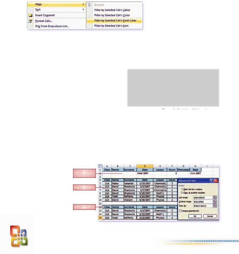
Figure 6.12: Popup menu, Filter options
Yet another faster way exists. Right click on the item that you want to filter and from the popup menu, select “Filter by selected cell’s value” or any other appropriate option. But with this method, you can filter according to one value. For more complex filtering, you should use the other methods.
6.3.2 Advanced Filter
The Advanced Filter command can filter a list in place like the AutoFilter command, but it does not display drop-down lists for the columns. Instead, you type the criteria by which you want to filter in a separate criteria range above the list. A criteria range allows for more complex criteria to be filtered.
The following wildcard characters can be used as comparison criteria for filters when filtering lists.
Example 6.3:
Operator |
Meaning |
|
|
? (question |
Any single character. For example, sm?th |
mark) |
finds “smith” and “smyth” |
* (asterisk) |
Any number of characters. For example, |
|
*east finds “Northeast” and “Southeast” |
~ (tilde) |
A question mark, asterisk, or tilde. For |
|
example, fy91~? finds “fy91?” |
|
Figure 6.13: Using Wildcards |
Your guidance teacher has a list of absences in a worksheet. He wants to analyze the list with questions like: show me the list of the students whose absences are between March and June and at the same time who have two hours from a lesson, etc. Help him to prepare the list.
Solution: You can apply an ‘Advanced filter’. You can write a condition for each column. After that, you can apply these conditions to your main range of data.
Advanced Filter can even copy the result onto another location. First, click the Advanced button from the Data tab, and then select your criteria range.
Finally click the “Copy to another location” radio button to activate the Copy to combo box, and then select the location where the result will be copied to.
Condition
Range
Data Range
Copy to
Figure 6.14: Advanced Filter
Data Processing |
109 |

6.4 Consolidating Worksheets
Consolidation means you summarize the information from several workbooks or worksheets using linked formulas into a worksheet. Here are two common examples of consolidation:
The budget for each department in your company is stored in a single workbook, with a separate worksheet for each department. You need to consolidate the data and create a company-wide budget on a single sheet.
Each department head submits a budget to you in a separate workbook file. Your job is to consolidate these files into a company-wide budget.
These types of tasks can be very difficult or quite easy. The task is easy if the information is laid out exactly the same in each worksheet. If the worksheets aren’t laid out identically, they may be similar enough. In the second example, some budget files submitted to you may be missing categories that aren’t used by a particular department. In this case, you can use a handy feature in Excel that matches data by using row and column titles using the Consolidate command in the Data Tab.
If the worksheets bear little or no resemblance to each other, your best bet may be to edit the sheets so that they correspond to one another. Better yet, return the files to the department heads and insist that they submit them using a standard format.
You can use any of the following techniques to consolidate information from multiple workbooks:
Use external reference formulas.
Copy the data and use Home Clipboard Paste Paste Link.
Use the Consolidate dialog box, displayed by choosing Data Data Tools Consolidate.
6.4.1 Consolidating worksheets by using formulas
Consolidating with formulas simply involves creating formulas that use references to other worksheets or other workbooks. The primary advantages of using this method of consolidation are
Dynamic updating—if the values in the source worksheets change, the formulas are updated automatically.
The source workbooks don’t need to be open when you create the consolidation formulas.
If you’re consolidating the worksheets in the same workbook and all the worksheets are laid out identically, the consolidation task is simple. You can just use standard formulas to create the consolidations. For example, to compute the total for cell A1 in worksheets named Sheet2 through Sheet10, enter the following formula:
=SUM(Sheet2:Sheet10!A1)
110 |
Microsoft Excel |