- •Preface
- •Contents
- •1 Introduction
- •1.1 Physics
- •1.2 Mechanics
- •1.3 Integrating Numerical Methods
- •1.4 Problems and Exercises
- •1.5 How to Learn Physics
- •1.5.1 Advice for How to Succeed
- •1.6 How to Use This Book
- •2 Getting Started with Programming
- •2.1 A Python Calculator
- •2.2 Scripts and Functions
- •2.3 Plotting Data-Sets
- •2.4 Plotting a Function
- •2.5 Random Numbers
- •2.6 Conditions
- •2.7 Reading Real Data
- •2.7.1 Example: Plot of Function and Derivative
- •3 Units and Measurement
- •3.1 Standardized Units
- •3.2 Changing Units
- •3.4 Numerical Representation
- •4 Motion in One Dimension
- •4.1 Description of Motion
- •4.1.1 Example: Motion of a Falling Tennis Ball
- •4.2 Calculation of Motion
- •4.2.1 Example: Modeling the Motion of a Falling Tennis Ball
- •5 Forces in One Dimension
- •5.1 What Is a Force?
- •5.2 Identifying Forces
- •5.3.1 Example: Acceleration and Forces on a Lunar Lander
- •5.4 Force Models
- •5.5 Force Model: Gravitational Force
- •5.6 Force Model: Viscous Force
- •5.6.1 Example: Falling Raindrops
- •5.7 Force Model: Spring Force
- •5.7.1 Example: Motion of a Hanging Block
- •5.9.1 Example: Weight in an Elevator
- •6 Motion in Two and Three Dimensions
- •6.1 Vectors
- •6.2 Description of Motion
- •6.2.1 Example: Mars Express
- •6.3 Calculation of Motion
- •6.3.1 Example: Feather in the Wind
- •6.4 Frames of Reference
- •6.4.1 Example: Motion of a Boat on a Flowing River
- •7 Forces in Two and Three Dimensions
- •7.1 Identifying Forces
- •7.3.1 Example: Motion of a Ball with Gravity
- •7.4.1 Example: Path Through a Tornado
- •7.5.1 Example: Motion of a Bouncing Ball with Air Resistance
- •7.6.1 Example: Comet Trajectory
- •8 Constrained Motion
- •8.1 Linear Motion
- •8.2 Curved Motion
- •8.2.1 Example: Acceleration of a Matchbox Car
- •8.2.2 Example: Acceleration of a Rotating Rod
- •8.2.3 Example: Normal Acceleration in Circular Motion
- •9 Forces and Constrained Motion
- •9.1 Linear Constraints
- •9.1.1 Example: A Bead in the Wind
- •9.2.1 Example: Static Friction Forces
- •9.2.2 Example: Dynamic Friction of a Block Sliding up a Hill
- •9.2.3 Example: Oscillations During an Earthquake
- •9.3 Circular Motion
- •9.3.1 Example: A Car Driving Through a Curve
- •9.3.2 Example: Pendulum with Air Resistance
- •10 Work
- •10.1 Integration Methods
- •10.2 Work-Energy Theorem
- •10.3 Work Done by One-Dimensional Force Models
- •10.3.1 Example: Jumping from the Roof
- •10.3.2 Example: Stopping in a Cushion
- •10.4.1 Example: Work of Gravity
- •10.4.2 Example: Roller-Coaster Motion
- •10.4.3 Example: Work on a Block Sliding Down a Plane
- •10.5 Power
- •10.5.1 Example: Power Exerted When Climbing the Stairs
- •10.5.2 Example: Power of Small Bacterium
- •11 Energy
- •11.1 Motivating Examples
- •11.2 Potential Energy in One Dimension
- •11.2.1 Example: Falling Faster
- •11.2.2 Example: Roller-Coaster Motion
- •11.2.3 Example: Pendulum
- •11.2.4 Example: Spring Cannon
- •11.3 Energy Diagrams
- •11.3.1 Example: Energy Diagram for the Vertical Bow-Shot
- •11.3.2 Example: Atomic Motion Along a Surface
- •11.4 The Energy Principle
- •11.4.1 Example: Lift and Release
- •11.4.2 Example: Sliding Block
- •11.5 Potential Energy in Three Dimensions
- •11.5.1 Example: Constant Gravity in Three Dimensions
- •11.5.2 Example: Gravity in Three Dimensions
- •11.5.3 Example: Non-conservative Force Field
- •11.6 Energy Conservation as a Test of Numerical Solutions
- •12 Momentum, Impulse, and Collisions
- •12.2 Translational Momentum
- •12.3 Impulse and Change in Momentum
- •12.3.1 Example: Ball Colliding with Wall
- •12.3.2 Example: Hitting a Tennis Ball
- •12.4 Isolated Systems and Conservation of Momentum
- •12.5 Collisions
- •12.5.1 Example: Ballistic Pendulum
- •12.5.2 Example: Super-Ball
- •12.6 Modeling and Visualization of Collisions
- •12.7 Rocket Equation
- •12.7.1 Example: Adding Mass to a Railway Car
- •12.7.2 Example: Rocket with Diminishing Mass
- •13 Multiparticle Systems
- •13.1 Motion of a Multiparticle System
- •13.2 The Center of Mass
- •13.2.1 Example: Points on a Line
- •13.2.2 Example: Center of Mass of Object with Hole
- •13.2.3 Example: Center of Mass by Integration
- •13.2.4 Example: Center of Mass from Image Analysis
- •13.3.1 Example: Ballistic Motion with an Explosion
- •13.4 Motion in the Center of Mass System
- •13.5 Energy Partitioning
- •13.5.1 Example: Bouncing Dumbbell
- •13.6 Energy Principle for Multi-particle Systems
- •14 Rotational Motion
- •14.2 Angular Velocity
- •14.3 Angular Acceleration
- •14.3.1 Example: Oscillating Antenna
- •14.4 Comparing Linear and Rotational Motion
- •14.5 Solving for the Rotational Motion
- •14.5.1 Example: Revolutions of an Accelerating Disc
- •14.5.2 Example: Angular Velocities of Two Objects in Contact
- •14.6 Rotational Motion in Three Dimensions
- •14.6.1 Example: Velocity and Acceleration of a Conical Pendulum
- •15 Rotation of Rigid Bodies
- •15.1 Rigid Bodies
- •15.2 Kinetic Energy of a Rotating Rigid Body
- •15.3 Calculating the Moment of Inertia
- •15.3.1 Example: Moment of Inertia of Two-Particle System
- •15.3.2 Example: Moment of Inertia of a Plate
- •15.4 Conservation of Energy for Rigid Bodies
- •15.4.1 Example: Rotating Rod
- •15.5 Relating Rotational and Translational Motion
- •15.5.1 Example: Weight and Spinning Wheel
- •15.5.2 Example: Rolling Down a Hill
- •16 Dynamics of Rigid Bodies
- •16.2.1 Example: Torque and Vector Decomposition
- •16.2.2 Example: Pulling at a Wheel
- •16.2.3 Example: Blowing at a Pendulum
- •16.3 Rotational Motion Around a Moving Center of Mass
- •16.3.1 Example: Kicking a Ball
- •16.3.2 Example: Rolling down an Inclined Plane
- •16.3.3 Example: Bouncing Rod
- •16.4 Collisions and Conservation Laws
- •16.4.1 Example: Block on a Frictionless Table
- •16.4.2 Example: Changing Your Angular Velocity
- •16.4.3 Example: Conservation of Rotational Momentum
- •16.4.4 Example: Ballistic Pendulum
- •16.4.5 Example: Rotating Rod
- •16.5 General Rotational Motion
- •Index
8.2 Curved Motion |
217 |
8.2 Curved Motion
We can use the insight from motion along a straight wire to understand curved motion, such as the circular motion of an atom in a rotating, rigid molecule or the motion of a roller-coaster car following its track.
Position
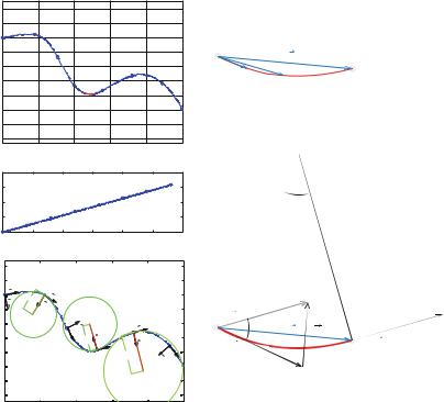
For a train running along a track as illustrated in Fig. 8.2 we can use the same description as we used above: We describe the position, r(s(t )), of the train by the distance, s(t ), travelled along the track. In Fig. 8.2 the train moves with constant speed along the track. A sequence of times at constant intervals, ti = i T , as shown with circles.
(A) |
40 |
|
|
|
|
|
|
|
|
|
|
|
|
|
|
|
|
|
20 |
|
|
|
|
|
|
|
|
(D) |
|
|
|
|
|
|
|
|
0 |
|
|
|
|
|
|
|
|
|
|
|
|
|
|
|
|
|
−20 |
|
|
|
|
|
|
|
|
|
|
|
|
r |
|
|
|
M] |
|
|
|
|
|
|
|
|
|
A |
|
|
|
|
|
|
|
−40 |
|
|
|
|
|
|
|
|
|
|
|
|
|
|
|
||
[ |
|
|
|
|
|
|
|
|
|
|
|
|
|
|
|
|
|
y |
−60 |
|
|
|
|
|
|
|
|
|
|
|
|
s |
|
A’ |
|
|
−80 |
|
|
|
|
|
|
|
|
|
|
|
|
|
|
|
|
|
|
|
A |
|
A’ |
|
|
|
|
|
|
|
|
|
|
|
|
|
|
|
|
|
|
|
|
|
|
|
|
|
|
|
|
||
−100 |
|
|
|
|
|
|
|
|
|
|
|
|
|
|
|
|
|
−120 |
|
|
|
|
|
|
|
|
|
|
|
|
|
|
|
|
|
−140 |
|
|
|
|
|
|
|
|
|
|
|
|
|
|
|
|
|
|
0 |
|
50 |
100 |
|
150 |
|
200 |
|
|
|
|
|
|
|
|
|
|
|
|
|
x [M] |
|
|
|
(e) |
|
|
|
B |
|
|
|
||
(b) 400 |
|
|
|
|
|
|
|
|
|
|
|
|
|||||
|
|
|
|
|
|
|
|
|
|
|
Δφ |
|
|
|
|||
[M] |
300 |
|
|
|
|
|
|
|
|
|
|
|
|
|
|
|
|
|
|
|
|
|
|
|
|
|
|
|
|
|
|
|
|
||
200 |
|
|
|
|
A’ |
|
|
|
|
|
|
|
|
|
|
|
|
s |
|
|
A |
|
|
|
|
|
|
|
|
|
|
|
|
|
|
|
|
|
|
|
|
|
|
|
|
|
|
|
|
|
|
||
|
100 |
|
|
|
|
|
|
|
|
|
|
|
|
|
|
|
|
|
00 |
|
5 |
10 |
|
15 |
20 |
25 |
|
30 |
|
|
|
|
|
|
|
|
|
|
|
|
t [S] |
|
|
|
|
|
|
|
|
|
|
|
|
(c) |
40 |
|
|
|
|
|
|
|
|
|
|
|
|
|
|
|
|
|
20 |
|
|
|
|
|
|
|
|
|
|
|
|
|
|
|
|
|
0 |
UT |
|
UT |
|
|
|
|
|
|
|
|
|
|
|
|
|
|
U |
ρ |
|
|
|
|
|
|
|
|
|
|
|
|
|
||
|
|
U |
|
|
|
|
|
|
|
|
|
|
|
|
|
|
|
|
−20 |
N |
|
|
|
|
|
|
|
|
|
t) |
|
|
|
|
|
|
|
N |
|
|
|
|
|
|
|
|
|
|
|
|
|
||
[M] |
|
|
|
|
|
|
|
|
|
|
|
(t+ |
|
|
|
|
|
−40 |
|
|
|
|
|
|
|
|
|
UT |
|
|
|
|
|
||
|
|
N |
|
|
|
|
|
|
|
Δφ |
r |
U |
|
|
|||
y |
|
|
|
U |
|
|
|
UT |
|
|
|
|
|
|
|
||
|
|
|
|
|
|
|
|
|
|
|
|
|
|
|
|
t) |
|
|
−60 |
|
|
U |
ρ |
UN |
|
|
|
A |
|
|
|
s |
T |
(t+ |
|
|
|
|
T |
|
U |
|
|
|
|
|
|
||||||
|
|
|
|
|
|
|
|
N |
|
|
U |
(t) |
|
|
UT |
|
|
|
−80 |
|
|
|
|
|
ρ |
U |
U |
|
|
|
|
A’ |
|
||
|
|
|
|
|
UT |
|
T |
|
|
|
|
||||||
|
|
|
|
|
|
|
|
N |
T |
|
|
|
|
|
|
|
|
|
−100 |
|
|
|
|
|
|
|
|
|
|
|
|
|
|
|
|
|
−120 |
|
|
|
|
|
|
|
|
|
|
|
|
|
|
|
|
|
−140 |
|
|
|
|
|
|
|
|
|
|
|
|
|
|
|
|
|
0 |
|
50 |
100 |
|
150 |
200 |
|
|
|
|
|
|
|
|
|
|
|
|
|
|
x [M] |
|
|
|
|
|
|
|
|
|
|
|
Fig. 8.2 Illustration of a motion along a curved path. a A train track. The train starts at r = 0 m at t = 0 s. Circles mark the positions at times ti . b Plots of the length s(t ) along the track. Circles indicate the times ti . c The velocity in A approaches a tangent to the line as the time interval t decreases. d Illustration of the change in tangential vector uˆ T . e Illustration of the velocity, acceleration, and normal vectors along the track, as well as the local curvature of the track illustrated
by the radius of the circles
218 |
8 Constrained Motion |
Velocity Vector
What is the velocity of the train? The velocity vector is the time derivative of the position vector:
v |
d r |
= |
lim |
|
r(t + |
t ) − r(t ) |
= |
lim |
|
r |
. |
(8.4) |
|||
|
|
|
|
||||||||||||
= d t |
0 |
|
t |
0 |
|
||||||||||
|
t |
→ |
|
t |
→ |
t |
|
||||||||
|
|
|
|
|
|
|
|
|
|
|
|
|
|
We see from Fig. 8.2c that as the time interval t decreases, the displacement r becomes tangential to the curve, just as we found in Chap. 6:
v(t ) = v(t )uˆ T , |
(8.5) |
where uˆ T (t ) is the unit tangent vector, uˆ T = v/|v|. We also see that as |
t becomes |
small, the arc length along the curve, s becomes approximately the same as the displacement r = | r|:
|
|
r → s when |
t → 0 . |
(8.6) |
||||||
The magnitude of the velocity therefore approaches |
|
|||||||||
|
= |
t |
= |
t |
→ |
t |
→ d t |
|
||
v |
|
| r| |
|
r |
|
s |
|
d s |
. |
(8.7) |
|
|
|
|
|
|
|
when t → 0. Now, we know both the direction and the magnitude of the velocity:
Velocity of motion along a curve: |
|
|
|
v(t ) = v(t ) uˆ T (t ) = |
d s |
uˆ T (t ) . |
(8.8) |
|
|||
d t |
Notice that the unit vector uˆ T is not a constant, but changes with time as the object moves: uˆ T = uˆ T (t ).
Acceleration Vector
The acceleration of the train can be found by taking the time derivative of the velocity vector:
a |
|
d |
v(t )u |
(t ) |
|
d v |
u |
|
v(t ) |
d uˆ T |
. |
(8.9) |
= d t |
|
+ |
|
|||||||||
|
ˆ T |
|
= d t ˆ T |
|
d t |
|
We recognize the first component as the rate of change of the magnitude of the velocity—this is how the speedometer changes as the train accelerates.
8.2 Curved Motion |
219 |
What about the second term? We have illustrated a small part of a motion in Fig. 8.2d. We are interested in the change in the tangent vector from the point A at r(t ) to the point A′ at r(t + t ). We have illustrated the tangent vectors, and in the small inset, we have illustrated the change in the tangent vectors, uˆ T . For a small increment t , we argue that the length of the uˆ T vector is approximately given as the length of the arc between the two tangent vectors, which is the angle Δφ between the two vectors multiplied by the length of the vectors, which is 1. Now, we can relate the angle Δφ to the local geometry of the curve by drawing a line A B normal to the tangent vector in A, and a line A′ B normal to the tangent vector in A′. This forms a triangle that is congruent with the small triangle formed by the tangent unit vectors, the angle spanned by the two lines A B and A B′ is therefore Δφ. The length of A B and A B′ is called the radius of curvature, ρ. The angle Δφ is also given as the arc
length from A to A′, which is the distance |
|
s along the trajectory, divided by the |
||
local radius ρ: |
|
|
|
|
Δφ = |
|
s |
. |
(8.10) |
|
|
|||
|
ρ |
The direction of the change in the unit tangent vector is toward the center of the circle, that is, toward the point B. We call this direction the normal direction, and we call the unit vector pointing in this direction for the unit normal vector, uˆ N . The change in the tangent vector is therefore:
|
|
s |
|
|
uˆ T = | |
uˆ T |uˆ N = Δφuˆ N = |
|
uˆ N . |
(8.11) |
ρ |
The time derivative of the tangent vector is therefore:
d uˆ T (t ) |
= |
lim |
|
u T |
= |
lim |
|
s |
u |
v(t ) |
1 |
u |
(t ) . |
(8.12) |
|||
d t |
0 |
t |
0 |
ρΔt |
ρ (t ) |
||||||||||||
t |
→ |
t |
→ |
ˆ N = |
|
ˆ N |
|
|
|||||||||
|
|
|
|
|
|
|
|
|
|
|
|
|
|
|
Now, we insert this expression back into the expression for the acceleration in (8.9), getting
a(t ) = |
d v |
uˆ T (t ) + |
v2(t ) |
uˆ N (t ) . |
(8.13) |
d t |
ρ (t ) |
||||
|
|
|
|
|
|
Here, we write that the radius of curvature, ρ (t ), is a function of time, because the radius of curvature is a function of the position along the curve, ρ (s), and the position along the curve for the object is a function of time, s = s(t ): ρ (t ) = ρ (s(t )).
We have therefore shown that the acceleration vector can be written as
a(t ) = aT (t ) uˆ T (t ) + aN (t ) uˆ N (t ) , |
(8.14) |
220 |
|
|
|
|
8 Constrained Motion |
where the tangential acceleration is |
|
|
|
|
|
|
d v |
|
|
|
|
aT (t ) = |
|
, |
(8.15) |
||
d t |
|||||
and the normal acceleration is |
|
|
|
|
|
aN (t ) = |
v2(t ) |
(8.16) |
|||
|
|
. |
|||
|
ρ |
The magnitude of the normal acceleration, aN = v2/ρ is often called the sentripetal acceleration of the object.
Uniform Circular Motion
These results can be simplified for uniform circular motion, where an object moves in a circle with a constant speed, v. In this case, the speed v(t ) does not change, and the radius of curvature is constant and equal to the radius, R, of the circle. The acceleration is therefore aN = v2/ R, directed in towards the center of the circle. This is illustrated by the motion diagram in Fig. 8.2.
Non-uniform Circular Motion
Figure 8.3 illustrates a motion diagram for a non-uniform circular motion: One case where the speed is increasing and one case where the speed is decreasing. In both cases, the radius of curvature is constant and equal to the radius, R, of the circle. The acceleration is therefore
|
d v |
v2 |
|
||
a = |
|
uˆ T + |
|
uˆ N . |
(8.17) |
d t |
R |
Angular Coordinates
We can also specify a position on the circle by the angle φ (t ) as illustrated in Fig. 8.3. How are the distance s(t ) and the angle φ (t ) related? The distance s(t ) corresponds to the arc length along the circle:
s(t ) = Rφ (t ) . |
(8.18) |
The two representations s(t ) or φ (t ) can both be used to represent the position, and you may use whatever representation you find most practical.
The speed can be related to the rate of change of the angle, φ, since
d s |
= |
d |
( Rφ (t )) = R |
d φ |
= Rω(t ) , |
(8.19) |
|
|
|
d t |
d t |
d t |