


96 |
5 Forces in One Dimension |
There are local variations of g along the Earth’s surface due to deviations of the spherical shape of the Earth, due to topographical variations, and due to differences in density in the Earth’s crust. In addition, there are variations in the effective g due to the rotation of the Earth. Surveys of variations in g due to density differences in the crust are used as a remote sensing technique that gives important information about the properties of rocks present in the Earth’s crust. This technique is routinely used for example for petroleum exploration.
5.6 Force Model: Viscous Force
You will often encounter objects that are in contact with a surrounding fluid such as a air or water. We therefore need a force model for the interaction between fluids and solid objects. Unfortunately, there is no fundamental law of nature for such an interaction. Instead, we must determine the force model from experiments or calculations based on an underlying model for fluid flow, and use this result as our model. Fortunately, experiments and calculations show that the force from the fluid has a simple form—it depends on the velocity of the object.
Drag Force at Low Velocities
If you pull a sphere through water, you expect a contact force FD from the water on the sphere counteracting the motion of the sphere relative to water because water is forced to flow around the sphere. Both experiments and theoretical models show that for low velocities the fluid flows smoothly around the object (see Fig. 5.7), and the force, FD , from the fluid is proportional to the velocity of the object relative to the fluid.
The viscous force on an object moving at a velocity v relative to a fluid is:
FD = −kvv , |
(5.17) |
where kv is a constant that depends on the objects size, shape and surface, as well as on the (dynamic) viscosity of the fluid. Stokes showed that at low velocities
kv = 6π η R , |
(5.18) |
where R is the radius of the sphere and η is the viscosity of the fluid. The viscosity of air is η = 1.82 × 10⁻⁵ Nsm−2 (at room temperature), and the viscosity of water is η = 1.00 × 10⁻³ Nsm−2 (at room temperature).

5.6 Force Model: Viscous Force |
97 |
y
2
1.5
u
1
0.5
Fv
0
-0.5
-1
-1.5
-2 |
|
|
|
|
|
|
-2 |
-1.5 -1 |
-0.5 0 |
0.5 |
1 |
1.5 |
2 |
x
y
2
1.5
u
1
0.5
0 |
Fv |
|
-0.5
-1
-1.5
-2
-2 |
-1.5 -1 |
-0.5 0 |
0.5 |
1 |
1.5 |
2 |
x
Fig. 5.7 Illustration of a drag force on an object due to the motion of the object relative to the surrounding fluid. At low velocities the fluid flow around the object is smooth, and the force is approximately proportional to the velocity. At higher velocities, the fluid flow becomes turbulent near the surface, the flow becomes irregular, and the force is approximately proportional to the square of the velocity
We call a force that is proportional to the velocity (of the object) a viscous force. If the force is a contact force from a fluid we also often use the term drag force to describe the interaction.
Drag Force at High Velocities
At larger velocities the fluid flow around the object becomes more irregular (see Fig. 5.7), and the drag force is not mainly related to the forces required to drag the fluid along the surface of the object, but instead depends on the under-pressure generated behind the object. In this case, the force is proportional to the square of the velocity, and we call this law the square law of air resistance.
The drag force on an object moving at a velocity v relative to a fluid is:
FD = −Dv2 , |
(5.19) |
acting in the direction opposite the velocity.
The minus sign shows that the force acts in the direction opposite the velocity. The prefactor D is a constant that depends on the objects size, shape and surface, and

98 |
5 Forces in One Dimension |
the density of the fluid. Experimental data gives an approximative value for D for a spherical object:
D 12.0 ρ R2 . |
(5.20) |
where ρ is the density of the fluid, and R is the radius of the sphere.
General Model for Fluid Drag
The behaviors for low and high velocities are special cases of a more general model for the drag force. Experiments show that the drag force can be written in the general form:
FD = |
1 |
ρ S C D (v, η, ρ , d)v2 , |
(5.21) |
2 |
where ρ is the density of the fluid. For air ρ = 1.293 kg/m3 at normal pressures and temperatures. S is the cross-sectional area of the object—that means the area of the object’s projection on a plane normal to the direction of motion. For a sphere with radius r the cross-sectional area is S = π r 2. The speed of the object relative to the fluid is v. The viscosity of the fluid is η, and d is a characteristic length scale, such as the diameter of a sphere. The coefficient C D (. . .) is called the drag coefficient and describes the details of the air resistance—the physics of drag is hidden in this function. For a given object type—such as a sphere of a given material—experiments show a remarkable feature: The drag coefficient only depends on one number, Re, called the Reynold’s number:
ρd |
v . |
(5.22) |
|
C D (v, η, ρ , d) = C D ( Re) , Re = |
|
||
η |
|||
This is a surprisingly compact description with many interesting implications. For example, if you increase the velocity by a factor 10 you get the same drag coefficient if you either reduce the radius by a factor 10 or increase the viscosity by a factor 10. The general function for the drag coefficient, C D ( Re), for a smooth sphere is shown in Fig. 5.8. (You can find the data-set for part (a) in cdreynolds.d5).
For small velocities, we expect to recover Stokes’ general result: FD = 6π η Rv, which implies that C D ( Re) Re−1 for small v (and Re). This is indeed what we observe in Fig. 5.8, where Re−1 is shown as a straight line. For large velocities, we see that the drag coefficient becomes approximately constant, and the force is therefore proportional to the square of the velocity. Our simplified models for small and large velocities are therefore consistent with the experimental results, and we
5http://folk.uio.no/malthe/mechbook/cdreynolds.
5.6 |
99 |
CD
103 |
|
|
|
|
|
|
|
|
|
|
|
|
|
Sphere |
|
|
|
|
|
|
Tilted cube |
||||
102 |
A |
|
|
|
|
|
|
|
|
|
|
|
|
|
|
|
|
|
|
||||||
|
|
|
|
|
|
|
|
|
|
|
|
|
|
|
|
|
|
||||||||
|
|
|
|
|
|
|
|
|
|
|
|
|
|
|
|
||||||||||
101 |
B |
|
|
|
|
|
|
|
|
|
|
|
CD ( v0 ) = 0.47 |
|
|
|
|
|
|
|
|||||
|
|
|
|
|
|
|
|
|
|
|
|
|
|
|
|
|
|
|
|||||||
|
|
|
|
|
|
|
|
|
|
|
|
|
|
|
|
|
CD ( v0 ) = 0.47 |
||||||||
100 |
|
|
C |
|
|
D |
|
|
|
|
|
|
|
|
|
|
|
|
|
|
|
|
|
|
|
|
|
|
|
|
|
|
|
|
|
|
|
|
|
|
|
|
|
|
|
|
|
|
|
|
|
10−1 |
|
|
|
|
|
E |
|
|
|
|
|
|
|
Cube |
|
|
|
|
|
|
|
|
|
Streamlined object |
|
|
|
|
|
|
|
|
|
|
|
|
|
|
|
|
|
|
|
|
|
|
|||||
|
|
|
|
|
|
|
|
|
|
|
|
|
|
|
|
|
|
|
|
||||||
10−2 |
|
|
|
|
|
|
|
|
|
|
|
|
|
|
|
|
|
|
|
|
|
|
|
|
|
|
|
|
|
|
|
|
|
|
|
|
|
|
|
|
|
|
|
|
|
|
|
|
|
|
|
|
|
|
|
|
|
|
|
|
|
|
|
|
CD ( v0 ) = 1.05 |
|
|
|
|
|
CD ( v0 ) = 0.04 |
||||||
10 |
0 |
2 |
10 |
4 |
10 |
6 |
|
|
|
|
|
|
|
|
|
|
|||||||||
|
|
|
|
|
|
|
|
|
|
|
|||||||||||||||
|
|
10 |
|
|
|
|
|
|
|
|
|
|
|
|
|
|
|
|
|
|
|
||||
Re
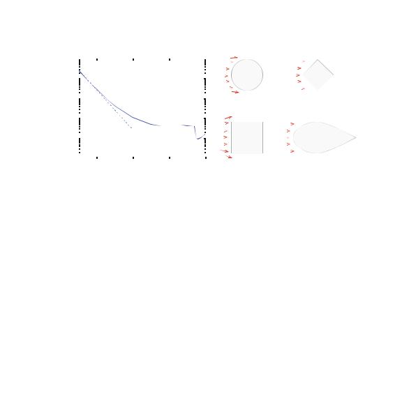
Fig. 5.8 a The drag coefficient C D as a function of Reynold’s number, Re = ρdv/η based on experimental data. b The drag coefficient C D at the same velocity for object with the same crosssectional area, but with different shapes
now also have a better understanding of what small and large means: Small means Re 1 and large means Re 1000.
Something strange happens when the Reynold’s number reaches Re = 3.2 × 10⁵: The drag coefficient drops significantly! A careful calculation (which you can program yourself) shows that not only the drag coefficient but also the fluid drag force falls. How can the drag force decrease when the velocity increases? This effect is due to boundary-layer turbulence (which we will not explain here). The transition point where this effect kicks in depends on surface properties of the object. For a rough surface, such as that of a golf ball, the transition occurs for a lower Reynolds number than for a smooth ball. This is the reason why golf balls have a rough surface: The air drag force for large velocities is reduced by this design.
What happened to aerodynamic design? This is also hidden in the drag coefficient. The value of the drag coefficient depends on the shape of the object, and more aerodynamic designs have lower drag coefficients for approximately the same crosssectional area, as illustrated in Fig. 5.8.
5.6.1 Example: Falling Raindrops
This example demonstrates how we can find the motion of an object subject to a constant force (gravity), and to a velocity-dependent force.
Raindrops are often as small as d = 1mm in diameter as they start falling. Here, we apply the structured problem-solving approach to find their velocity, first without air resistance, and then with a model for viscous drag.
Sketch and Identify: We always start addressing a problem through a sketch which should include the system, a raindrop, the environment, and a coordinate system (see Fig. 5.9). We describe the position of the raindrop by its vertical position y(t ) as a function of time t .

100
Fig. 5.9 Left Illustration of a raindrop falling down. Right Free-body diagram for the drop. (Notice that a real raindrop is neither perfectly spherical nor “drop-shaped”, it is pushed flat by the air resistance force)
5 Forces in One Dimension
y |
|
|
|
|
|
y |
|
FD |
||||||
|
|
|
|
|
||||||||||
y0 |
|
|
|
|
|
v |
= 0 |
|
|
|||||
|
|
|
|
|
|
|
|
|
|
|
|
|||
|
|
|
|
|
|
0 |
|
|
|
|
|
|
|
|
y1 |
|
|
|
d |
|
|
|
|
|
|
|
|
|
v |
|
|
|
|
|
|
|
|
|
|
|||||
|
|
|
|
|
|
|
|
|
|
|
|
|
||
|
|
|
|
|
|
|
v1 |
|
|
|
||||
|
|
|
|
|
|
|
|
|
|
|
||||
|
|
|
|
|
|
|
|
|
|
|
||||
|
|
|
|
|
|
|
|
|
|
|
||||
|
|
|
|
|
|
|
|
|
|
|
|
|||
|
|
|
|
|
|
|
|
|
|
|
G |
|||
|
|
|
|
t0 |
|
t1 |
t |
|||||||
|
|
|
|
|
|
|
|
|
||||||
Model: The motion of the raindrop is determined by the forces acting on it. We draw the forces in a free-body diagram, as illustrated in Fig. 5.9. The sketch shows that the raindrop is only in contact with the surrounding air, which gives rise to an air resistance force FD . In addition, the raindrop is affected by gravity, G, from the Earth.
We have force models for each of these forces. We know that gravity is G = −mgj, where m is the mass of the raindrop. For the air resistance FD we assume that we can use the viscous law:
FD = −kvv(t ) j , |
(5.23) |
where v(t ) is the velocity of the drop. You should check with yourself that this force indeed has the correct sign. Remember that when the drop falls downward its velocity is negative.
Newton’s second law: We apply Newton’s second law to find the acceleration of the drop:
Fnet = FD + G = −mg j − kvv(t ) j = ma j , |
(5.24) |
which corresponds to
− mg − kvv(t ) = ma . |
(5.25) |
We lack two of the numbers in this equation: m and kv. We can find the mass of the drop by assuming that it is spherical and made of water. The volume of a sphere is V = (4π /3)r 3, where r = d/2 is the radius of the sphere, and the mass density of water is ρ = 1000.0 kg/m3. The mass of the drop is therefore
3
m = ρ V = ρ 4π r 3 = ρ 4π d = 5.24 × 10⁻⁷ kg . (5.26)
33 2
We find kv from Stokes’ formula in (5.18): kv = 6π Rη. The radius of the raindrop
is r = 0.5 × 10⁻³ m, and the viscosity of the air is η = 1.82 × 10⁻⁵ Nsm−2. This gives kv = 1.85 × 10⁻⁷ Nsm−1.

5.6 Force Model: Viscous Force |
101 |
Finally, to calculate the motion of the drop, we need to know its initial conditions: It starts from y(0) = h at t = 0 s at rest, that is, with v(0) = 0 m/s.
Simplified model: No air resistance: First, what happens in the simplified case when we have no air resistance? In that case, kv = 0, and the acceleration is a constant
a = −g . |
(5.27) |
|
We find the velocity as function of time by direct integration: |
|
|
v(t ) − v(0) = |
t |
(5.28) |
a dt = −gt . |
||
0
This corresponds to a free fall, as we have seen previously. We expect this to only be a good approximation as long as the air resistance term is small, that is as long as kvv(t ) is much smaller than mg, that is when
k |
v |
|
mg |
|
v |
mg |
|
5.24 × 10⁻⁷ kg 9.8 m/s2 |
|
27.8 m/s. |
(5.29) |
||
|
|
|
|
|
|
||||||||
|
|
kv |
= |
1.85 × 10⁻⁷ Nsm−1 |
|
||||||||
v |
|
|
|
|
|
||||||||
We will check how good this approximation is further on.
Simplified model: Constant velocity: What will happen as the drop starts to fall? It starts from zero velocity, hence the initial acceleration will be a = −g − (kv/m)v = −g. As the drop falls, the velocity becomes a negative number, but with increasing magnitude. The acceleration, a = −g − (kv/m)v will therefore approach zero. However, if the acceleration becomes zero, the velocity will no longer change, and the drop will have reached a stationary velocity—a velocity that does not change with time. This occurs when
kv |
|
|
|
kv |
mg |
|
||||
a = −g − |
|
v = 0 |
−g = |
|
v v = − |
|
. |
(5.30) |
||
m |
m |
kv |
||||||||
We call this velocity the terminal velocity, vT : |
|
|
|
|
||||||
|
|
|
mg |
|
|
|
(5.31) |
|||
|
|
|
vT = |
|
. |
|
|
|
||
|
|
|
kv |
|
|
|
||||
We therefore expect the drop to approach the velocity v = −vT as time increases.
Full model: Numerical solution: We now know both the initial behavior, a = −g, and the asymptotic behavior, a → 0 m/s2, v → −vT . We can find the velocity by solving
a = |
dv |
= −g − |
kv |
v , |
(5.32) |
|
|
dt m
102 |
5 Forces in One Dimension |
with initial conditions v(t0) = 0 m/s using Euler’s method:
v(ti + t ) = v(ti ) + t · a(ti , v(ti )) . |
(5.33) |
This method is implemented in the following program:
from pylab import *
#
# Physical variables g = 9.81
kv = 1.85e-7 # Nsmˆ-2 m = 5.2e-7 # kg time = 20.0
dt = 0.001
#Initial conditions v0 = 0.0
#Numerical initialization n = int(round(time/dt))
v = zeros(n,float) a = zeros(n,float) t = zeros(n,float)
#Set initial values
v[0] = v0
# Integration loop for i in range(n-1):
a[i] = -g - (kv/m)*v[i] v[i+1] = v[i] + a[i]*dt t[i+1] = t[i] + dt
Analysis of numerical solution: The resulting plot of v(t ) and a(t ) is shown in Fig. 5.10. We see that both v(t ) and a(t ) behaves as we expected. The drop starts with zero velocity and an initial acceleration of −g. The acceleration reduces as the velocity increases and the drop reaches a stationary state where it moves with constant velocity. We compare with the two simplified models. The behavior without air resistance is plotted as a dashed line, and it is indeed a reasonable approximation for small velocities, that is when |v| vT = 27.5 m/s. For long times the velocity approaches v → −vT , which is illustrated by the dotted line in the plot. The simplified solutions are therefore useful to check if our numerical solution is correct.
Full model: Analytical solution: Now that we have both found the simplified and the numerical solution, we are ready to attempt an analytical soultion. In this case
Fig. 5.10 Plot of v(t ) and a(t ) for the drop
a [m/s2] v [m/s]
0 |
|
|
|
|
-10 |
|
|
|
|
-20 |
|
|
|
|
-30 |
|
t [s] |
|
|
0 |
|
|
|
|
-5 |
|
|
|
|
-10 |
|
|
|
|
0 |
5 |
10 |
15 |
20 |
t [s]
5.6 Force Model: Viscous Force |
103 |
we are fortunate, since the particular equation in (5.32) can be solved analytically using separation of variables. We simplify the equation by writing:
dt |
= −g − m v = −g − vT v = −g |
1 + vT |
, |
(5.34) |
||||
dv |
|
kv |
|
g |
|
v |
|
|
with initial condition v(0) = 0 m/s. We separate v and t on each side of the equation:
|
|
|
|
|
|
|
|
|
|
|
|
|
|
|
|
dv |
|
|
= −gdt , |
|
|
|
|
(5.35) |
|||||
|
|
|
|
|
|
|
|
|
|
|
|
|
|
|
|
|
|
|
|
|
|||||||||
|
|
|
|
|
|
|
|
|
|
|
|
|
1 + v/vT |
|
|
|
|
|
|||||||||||
and integrate each side from t0 = 0 to t : |
|
|
|
= − |
|
|
|
|
|
|
|||||||||||||||||||
|
|
|
|
|
|
|
|
|
|
|
v(t ) |
1 |
|
dv/v |
|
|
|
t |
gdt . |
|
|
(5.36) |
|||||||
|
|
|
|
|
|
|
|
|
|
|
|
|
|
|
|
|
|
v |
|
|
|
|
|
|
|
|
|
|
|
|
|
|
|
|
|
|
|
|
|
|
v0 |
|
|
|
|
+ |
|
|
T |
0 |
|
|
|
|
|
|
|||
We introduce u = 1 + v/vT , du = dv/vT , dv = vT du: |
|
= −gt , |
|
||||||||||||||||||||||||||
1 |
+ |
|
|
|
vT |
u |
= −g(t − 0) |
vT ln 1 + vvT |
(5.37) |
||||||||||||||||||||
|
1 |
|
|
v(t )/vT |
du |
|
|
|
|
|
|
|
|
|
|
|
|
|
|
|
|
(t ) |
|
|
|
||||
ln 1 |
|
|
v |
|
|
|
v |
|
|
, 1 |
|
|
|
vv |
|
|
|
|
|
e−gt /vT |
|
|
v(t ) |
|
vT e−gt /vT |
1 . |
|||
|
+ |
|
v(t ) |
|
= − |
gt |
+ |
|
(t ) |
= |
|
|
= |
|
− |
||||||||||||||
|
|
|
|
T |
|
T |
|
|
T |
|
|
||||||||||||||||||
(5.38) Full model: Symbolic solution: You can solve (5.34) using the symbolic solver in Python. First, we define the variables g, u (corresponding to VT ) and v(t)
>>from sympy import *
>>v = Function(’v’)
>>from sympy.abc import t
>>from sympy.abc import g
>>from sympy.abc import u
Python can then solve the equation with the initial condition by
>> dsolve(Derivative(v(t),t)+g+g/u*v(t),v(t)) v(t) == C1*exp(-g*t/u) - u
This corresponds to the solution
v(t ) = vT e−gt /vT − 1 . |
(5.39) |
In most cases, machines are much better than humans at integration. In your career as a physicist it is therefore more important to be able to formulate problems so that they can be solved numerically or symbolically than to be able to solve them analytically yourself.
Test your understanding: What would happen if the drop started with a velocity v0 = −2vT ?