

reading / British practice / Vol D - 1990 (ocr) ELECTRICAL SYSTEM & EQUIPMENT
.pdfElectrical system monitoring and interlocking schemes
11 kV STATION BOARD 7B (88)
.m=m1=7■==
El3 |
11;3 3kV |
|
CHLORINATION |
|
|
TRANSFORMERPLANT |
7 (8) |
KEY EXCHANGE BOX |
|
|
°9 |
]‘/NITr |
Y |
C A |
Y |
3.3kV CHLORINATION(LIPLANT BOARD 7 (8) Ell A rf
1133.3kV/ 415V CHLORINATION
PLANT TRANSFORMER 7 (8)
415V CHLORINATION PLANT BOARD 7 (8)
Jic5
3.3kV CHLORINATION
PLANT BOARD 8 (7)
FIG. 1.59 Typical coded-key maintenance interlocking scheme
at least one of the Type A2 keys to satisfy the Safety Rule earthing requirements.
(h)Reinstatement of supplies will be established in the reverse order.
Note: It has been assumed that the Chlorination Plant Electrolysers are 'dead end feeders' in the above procedure.
8.6 Other safety interlocking
During normal operation it is imperative that all
equipment which contains live metal must be designed such that access is denied at all times whilst the equipment is energised. Typical examples of this are switchgear cubicles where internal access is not possible when the isolator is 'on', which is done by ensuring that in this position the door cannot be opened. Although these requirements are written in the equipment specification, there are several ways to achieve the objective. The choice must be one of a balanced design, preventing defeat from the unintentional act but at the same time not building in complications which makes normal operation more difficult.
83

CHAPTER 2
Electrical system analysis
1 Principles of electrical system analysis
1.1Introduction
1.2System design assessments
1.3Analysis program developments
1.4Analysis techniques
1.4,1 Reliability evaluation
1.4.2 Power system performance analysis 1.5 Quality assurance of analysis programs
2 Reliability evaluation of power systems
2.1Introduction
2.2Quantitative reliability evaluation
2.2.1Choice of numerical indices
2.2.2Scope of reliability evaluation assessments
2.3Computer programs for reliability evaluation
2.3.1Batch program — RELAPSE
2.3.2Interactive program — GRASP (Version 11
2.3.3Interactive program — GRASP (Version 21 2.4 Data requirements
2.4.1Active failure rate
2.4.2Passive failure rate
2.4.3Total failure rate
2.4.4Average repair time
2.4.5Switching time
2.4.6Maintenance rate
2.4.7Maintenance time
2.4.8Stuck probability
2.4.9Time limit of a limited energy source
2.4.10Common mode failure rate
2.5 Techniques employed
2.5.1 Graphical representation of the station electrical System
2.5.2Component and branch numbering
2.5.3Branch definition
2.5.4Criteria of failure
2.5.5Analysis control procedures
2.5.6Deduction of minimal paths
2.5.7Deduction of minimal cut sets 2.5,8 Types of failure/restoration event
2.5.9Switching effects of component active failure
2.5.10Markov state-space models
2.5.11Evaluation techniques (busbar indices)
2.5.12Evaluation techniques (system indices)
2.5.13Presentation of results
2.6Quality assurance
2.7Typical applications
2.7.1Example of the calculation and use of busbar indices
2.7.2Example of the calculation and use of system indices
3 Power system performance analysis
3.1Load flow analysis
3.1.1Introduction
3.1.2Program construction [4,5]
3.1.3Use of programs
3.2Fault level analysis
3.2.1Introduction
3.2.2Program construction
3.2.3Use of programs
3.3Stability analysis
3.3.1Introduction
3.3.2Analytical and programming considerations
3.3.3Use of programs
3.4Future developments of electrical analysis programs
4 References
1 Principles of electrical system analysis
1.1 Introduction
The assessment and validation of electrical power systems in terms of their predicted performance and comparative levels of reliability and availability are essential tasks in the early design phases for all major projects. This is particularly important in respect of those aspects of the design and performance necessary for ensuring the safe and satisfactory integration of various types of power station into the CEGB grid supply system.
Broadly, the primary functional design objectives of electrical system analysis are to:
• Ensure that the designs for plant and system net-
works comply with specified operating performance and safety criteria.
•Evaluate the comparative performance and cost effectiveness of alternative plant designs and system configurations.
•Determine and optimise plant and system parameters for technical performance specification purposes.
•Provide the electrical characteristics necessary for the design of electrical protection systems.
•Define system and plant constraints for operational and maintenance procedural purposes.
System and plant parameters are Currently fully represented by mathematical models in the design process
84
|
|
Principles of electrical system analysis |
|
|
|
|
|
a nd, with the evolution of digital computer aided design |
• Data tables are generated automatically from the |
||
diagram information for each of the plant com- |
|||
|
facilities over the past fifteen years, the scope and |
||
detailed representation of Dower system simulation |
ponents and system connections. |
||
studies has increased significantly in comparison with |
• Self-explanatory help and option menus are dis- |
||
earlier analysis techniques. Also, with the increasing |
|||
played on the screen and, where necessary, specific |
|||
involvement of computers, there are continuing pos- |
|||
error messages or warnings are displayed. |
|||
sibilities for the development and enhancement of the |
|||
• Display options allow key results to be displayed |
|||
computer programs described later in this chapter. |
|||
|
|
either directly on the network diagram or in tabular |
|
|
|
and graphical form. |
|
|
1 1 System design assessments |
The programs' user-friendly' operating procedures |
|
The design and operation of power systems require |
|||
are particularly enhanced by the extensive application |
|||
comprehensive analysis in order to evaluate the per- |
|||
of computer graphics for the input of system and |
|||
|
formance under normal and abnormal conditions of |
||
|
plant data, results output and control functions. Typi- |
||
operation, whilst recognising the defined system per- |
|||
cal examples of system network diagrammatic and |
|||
|
formance and safety criteria discussed in Chapter 1. |
||
|
graphical output displays that are capable of being |
||
|
In this regard, both power system performance and |
||
|
copied by means of a hard copy unit directly from |
||
reliability evaluation analysis play equally important |
|||
the computer terminal screen are shown in Figs 2.1 |
|||
roles in achieving a high standard of overall power |
|||
and 2.2. |
|||
system integrity and ensuring the optimal utilisation of |
|||
Experience in the collaborative development of com- |
|||
capital investment in power station plant and systems. |
|||
puter aided system analysis programs, has demonstrated |
|||
System integrity is particularly important for nuclear |
|||
that the final quality is particularly influenced by how |
|||
power stations, for which nuclear safety and district |
|||
well the design concepts, needs objectives, and organ- |
|||
hazard assessments have to be made in support of the |
|||
isational and responsibility arrangements are jointly |
|||
application for an operating licence. |
|||
established at the inception of the development project. |
|||
|
The design assessments must necessarily involve the |
||
|
Particular emphasis is therefore placed on the design |
||
reliability evaluation and power system performance |
|||
concepts and objectives being formulated on a sound |
|||
analysis of the interface connections between the grid |
|||
technical basis, while ensuring that associated important |
|||
system and the power station, together with the station |
|||
design functions, such as program structure, controls, |
|||
electrical systems which provide electrical power to the |
|||
mathematical models, calculation routines, data-base |
|||
boiler/reactor, turbine-generator auxiliaries and station |
|||
management, etc., are clearly defined. To assist further |
|||
services plant. The station electrical systems comprise |
|||
in the definition and understanding of the overall |
|||
many supply systems of the radial type, including |
|||
program logic, flow charts (typically as depicted in |
|||
transformers, switchgear, motors, gas turbine and diesel |
|||
Fig 2.3) are produced at the commencement of each |
|||
generators, cables and connections. |
|||
development project. The chart displays all the activities |
|||
|
|
||
|
|
which need to be considered in the development of a |
|
1.3 Analysis program developments |
new program and provides the starting point for the |
||
computer software program designer. |
|||
Power system analysis involves some very complex |
The further development of computer aided analysis |
||
numerical processes which, together with the entry of |
programs is an ongoing task in order to keep abreast |
||
system data and the extraction of essential results, |
with the rapid technological advances being made in |
||
constitute a very substantial workload on the design |
plant and system designs, e.g., the introduction of |
||
engineer in making assessments of system performance. |
modern electronic speed and voltage controllers for |
||
It is important, therefore, that aspects of computing |
governors and automatic voltage regulators (AVRs), |
||
organisation such as operating procedures and com- |
thyristor drive controllers, vacuum switches, fast op- |
||
mands are removed, as far as practicable, from the |
erating electronic protection equipment, etc. |
||
design engineer's tasks to enable him to concentrate |
|
||
on the quality of the system design and performance. |
|
||
|
To this end, separate suites of batch mode and |
1.4 Analysis techniques |
|
interactive computer programs have been specifically |
Prior to the development of the computer analysis |
||
developed to incorporate the following 'user-friendly' |
|||
facilities described in the previous section, hand calcula- |
|||
features: |
|||
tions formed the main method of analytical solution; |
|||
• System networks are drawn on the computer ter- |
|||
these were supported, whenever possible, by AC and |
|||
|
minal screens in diagrammatic form, thereby pro- |
DC analyser facilities for system load flows, fault levels |
|
|
viding a familiar framework for the engineer to |
and transient fault performance. |
|
|
identify the correctness of the system for analysis |
Such analysis techniques were inherently time con- |
|
|
purposes. |
suming and permitted only simplified representations |
|
|
|
||
85
Electrical system analysis |
Chapter 2 |
|
|
LOAD |
rLow |
RESULTS - BUSBAR PU VOLTS & LINE MVP |
|
|
|
|
|||||||||||||||||||||||||||||
|
|
|
LOCOING |
||||||||||||||||||||||||||||||||
|
|
|
|
|
|
|
|
|
|
|
|
|
|
|
|
|
|
|
|
|
|
|
|
|
|
|
|
|
42 |
|
|
e ileev |
|||
|
|
|
|
|
|
|
|
|
|
|
|
|
|
|
|
|
L511„ |
|
|
|
|
||||||||||||||
|
|
|
|
|
|
|
|
132KV |
|
|
|
|
|
|
|
|
|
|
|
|
|
|
|||||||||||||
|
|
|
|
|
|
|
|
|
|
|
|
|
|
|
|
|
|
|
|
|
|||||||||||||||
|
|
|
|
|
|
|
|
1.008 |
|
|
|
|
|
|
|
|
|
|
|
|
|
|
|
|
|
|
|
|
|
|
82.6, |
||||
|
|
|
|
|
|
|
|
|
|
|
|
|
|
|
|
|
|
|
|
|
|
|
|
|
|
|
|
|
|
|
|||||
|
|
|
|
|
|
|
|
233 4 |
|
|
|
|
|
|
|
|
|
|
|
|
|
|
|
|
|
|
|
145 |
|
|
|
|
|
|
|
|
|
|
|
|
|
|
|
|
|
|
|
|
|
|
|
|
|
|
|
|
|
|
|
|
|
|
|
|
|
|
|
|
|
|
|
|
|
|
|
|
|
|
|
|
|
|
|
|
|
|
|
|
|
|
|
|
|
|
|
|
|
|
|
|
|
|
|
|
|
|
|
|
|
|
|
|
|
|
|
|
|
|
SI |
|
|
|
|
|
|
|
|
|
|
|
|
|
|
|
|
|
|
|
|
|
|
|
|
|
|
|
|
|
|
|
|
|
|
|
|
|
341 |
|
|
|
|
|
|
|
|
|
|
|
|
|
|
|
|
|
|
|
|
|
|
|
|
|
|
|
|
|
|
|
|
|
|
|
|
|
|
|
|
|
|
|
|
|
|
|
|
|
|
|
|
|
|
|
|
|
|
|
|
|
|
|
|
|
|
|
|
|
|
|
1.052 |
|
|
|
|
|
|
|
|
|
|
|
|
|
|
|
|
|
|
|
|
|
|
|
|
|
|
|
|
|
|
|
|
|
|
|
|
|
|
J2 |
|
|
|
|
|
|
|
|
|
|
|
|
|
|
|
|
|
|
|
|
|
|
|
|
|
|
|
|
|
|
|
|
|
|
|
1.021 |
|
|
|
|
|
|
|
|
|
|
|
|
|
|
|
|
|
|
|
|
|
|
|
|
|
|
|
|
|
|
|
|
|
|
|
|
|
|
|
|
|
|
|
|
|
|
|
|
|
|
|
J3 |
|||
|
BSA |
28 |
1,... |
|
|
|
|
|
|
|
|
21' |
|
|
|
|
|
|
|
|
|
|
|
|
|
|
|
|
1.005 |
|
|||||
|
|
|
|
|
|
|
|
|
|
|
|
|
|
|
|
|
|
|
|
, |
|
|
|
|
|||||||||||
|
|
|
|
|
|
|
|
|
|
|
|
|
|
|
|
|
|
|
|
|
|
|
|
|
|
|
|
|
|||||||
|
1.011 |
|
|
|
... |
|
|
|
|
|
|
BSB |
|
|
|
|
.., |
|
|
|
|
|
|
|
|
|
|
BSC |
|||||||
|
|
|
|
|
|
|
|
|
|
|
|
|
|
|
|
|
|
|
|
|
|
|
|
|
|
|
|
|
|
||||||
|
' |
|
|
,---67-e------- ,,, |
|
|
|
|
6 . |
|
|
|
|
|
|
|
|
- |
,..... 7.. --S. -24. --•■•■•••!... |
|
1.003 |
||||||||||||||
I3 |
|
.---, |
|
—G |
|
|
|
. |
|
|
|
|
e.1 |
—pp, G — 6.7 |
|
|
|
|
4. |
|
|
|
|||||||||||||
|
7 |
.."--.. |
|
|
|
G - |
2.54 |
6.3-2.a |
|
|
0.i' |
|
|
|
|
|
|
|
|
|
|
|
|
|
|||||||||||
|
|
|
|
|
|
|
|
|
|
|
|
|
|
|
|
|
|
|
|
|
|
|
|
|
|
||||||||||
|
|
|
|
|
|
|
|
|
|
|
|
|
|
|
|
|
|
|
|
|
|
|
|
|
|
|
|
|
|
|
|
||||
|
|
|
|
Len |
7 |
|
|
|
J6 |
2.24 |
|
1.020 °•Sq 1.020 |
|
e.4 |
|
|
|
|
|
||||||||||||||||
|
|
|
|
|
|
|
|
|
|
|
|
|
1.020 G — |
|
|
|
|
|
|
|
|||||||||||||||
|
|
|
|
|
|
|
|
|
|
|
|
|
|
|
|
|
|
|
|
|
|
|
|
|
|
|
|
|
|
|
|
|
|||
|
|
|
|
|
|
|
|
|
|
|
|
|
|
|
|
|
|
|
|
|
|
|
|
|
|
|
|
|
|
|
|||||
|
|
|
|
|
|
|
|
|
|
|
|
|
|
|
|
|
|
|
J13 |
|
|
|
|
|
|
|
|
|
|
|
|
||||
|
|
, JI2 |
|
|
|
|
|
|
|
|
|
|
|
|
|
|
|
|
|
|
|
|
|
|
|
||||||||||
|
|
|
|
|
|
|
|
|
|
|
|
|
|
|
|
|
|
9 J14 |
|
|
|||||||||||||||
|
|
|
|
|
|
|
|
|
|
|
|
|
|
|
|
|
|
|
|
|
|
|
|
||||||||||||
|
|
|
|
|
|
|
|
|
|
|
|
|
|
|
|
|
|
|
1.006 |
|
|
|
|
|
|
|
|
||||||||
|
|
|
|
8.999 |
|
|
|
|
|
|
|
|
|
|
|
|
|
|
B6C |
1- . 011 |
|
|
|||||||||||||
|
|
|
|
|
|
|
|
|
|
|
|
|
|
|
|
|
|
|
|
||||||||||||||||
|
|
|
|
|
|
|
|
|
|
|
|
|
|
|
|
|
|
|
|||||||||||||||||
|
|
|
|
|
|
|
|
|
|
|
|
|
|
|
|
|
|
|
|
|
|
|
|
|
|
1.809 |
|
|
|
|
|
|
|
|
|
|
|
|
|
|
|
|
|
|
|
|
|
|
|
|
|
|
|
|
|
|
|
|
|
|
|
|
|
|
|
|
|
|
|
|
|
|
|
|
|
|
|
|
|
|
|
|
|
|
|
|
|
|
|
|
|
|
|
|
|
|
|
|
|
2.41 |
|
|
|
|
|
||
|
|
P/136AX |
86AY |
868Y |
|
BGBX |
|
|
0.998 |
|
|||
|
|
, |
8.998 |
.7.40.---44.11.4143154 |
74 |
1.008 |
|
|
|
|
mr■p. |
||
|
|
|
|
|
|
I |
|
|
|
|
|
|
|
• e.40 |
|
8 |
|
• * 0• |
||
|
|
|
|
|
||
|
|
|
. |
|
||
|
|
8 |
|
|||
|
|
|
|
|
||
|
|
|
ES |
|||
|
|
|
|
|
|
|
DSL |
|
|
|
|
||
0.998 1 |
|
|
|
|
|
|
|
|
|
|
|
|
|
|
|
|
4151.19 |
|||
|
|
|
|
|
|
|
|
|
|
|
0.54 |
|
|
|
|
|
!MCI' |
|
|
|
|
|
|
|
||
|
|
|
|
|
|
B6CX |
||||||
|
|
|
|
|
|
|
|
|
||||
|
|
|
1 i |
|
|
1.0113 |
||||||
|
|
■Lt' fl. |
|
|
|
|
|
|||||
|
|
|
|
|
|
|
||||||
,-- |
0 4. |
/) |
|
|
|
|
|
|
|
|
||
|
|
|
|
0 |
|
|
|
|
|
|||
, , r" |
|
|
e |
|
0.4 |
|
|
|||||
E — |
8,V' |
|
|
|
|
|
|
|||||
|
|
|
|
|
|
|
||||||
|
|
|
|
|
|
|
|
|
|
|
|
|
|
|
/ EN |
|
|
|
|
|
|
|
|||
Q.9 |
|
|
|
|
|
|
|
|
|
|
||
|
|
|
|
|
|
|
|
|
|
|
|
|
|
|
|
|
|
|
1151/0 |
|
|
|
|
|
|
|
|
|
|
4 |
1.035 |
|
|
|
|
|
||
|
|
|
|
0.7 . |
|
|
|
|
|
|
|
|
|
|
|
|
|
|
|
|
|
|
|
|
|
|
|
|
|
|
|
|
|
|||||||
|
|
|
|
|
|
|
|
|
|
|
66 % |
|
JU |
|
|
|
|
|
|
||||||||
|
|
|
|
|
|
|
|
|
|
|
|
|
|
|
|
|
|
|
|
|
|
|
|
|
|
|
|
660, |
|
|
|
|
|
|
|
|
|
|
|
|
|
|
|
|
|
|
|
||||||||
|
|
|
|
|
|
|
|
|
|
|
|
|
|
|
|
|
|
|
|
|
|
|
|
|
|
|
|
|
|
|
|
|
|
23.5KV |
|
|
|
|
|
|
|
|
|
|
|
|
|
|
|
|
|
||||
|
|
|
|
|
1,905 |
|
|
|
|
|
|
|
|
|
|
|
|
|
|
|
|
|
|||||
|
|
|
|
|
|
|
|
|
|
|
|
|
|
|
|
|
|
|
|
|
|
|
|
|
|
||
25 |
|
|
|
|
|
|
|
|
|
|
|
|
|
|
|
|
|
|
|
|
|||||||
|
|
|
|
|
|
|
|
|
|
|
|
|
|
|
|
|
|
|
|
|
|
|
|
|
|
|
|
|
|
|
|
|
|
|
|
|
|
|
|
|
|
9 |
|
|
J4 |
|
|
|
|
|
|||||
|
|
|
|
|
|
|
|
|
|
|
|
|
|
|
|
|
|
1.019 |
|
|
|
|
|
|
|||
|
|
|
|
|
|
|
|
|
|
|
|
|
|
|
|
550 |
|
|
|
|
|
|
|
|
|||
|
|
|
|
|
|
|
|
|
|
|
|
|
|
|
|
.01 |
|
|
|
|
|
|
|
11KV |
|||
|
|
|
|
|
|
|
|
|
|
|
|
|
|
|
|
|
|
|
|
|
|
|
|
|
|
|
|
|
|
|
|
|
|
|
|
|
|
|
|
|
|
|
|
|
|
r |
—c |
|
|
|
|||||
|
|
|
|
|
|
|
|
|
|
|
|
|
|
|
|
|
|
|
|
|
|
|
|
|
|
||
|
|
|
|
|
|
|
|
|
|
|
|
|
|
|
|
|
|
|
|
|
|
|
|||||
|
|
|
|
|
|
|
|
|
|
|
|
|
|
|
|
|
|
|
|
0 |
|
J11 |
|||||
|
|
|
1.A |
|
|
|
|
|
|
|
|
||||||||||||||||
|
|
|
|
|
|
|
|
|
|
|
|
|
|
|
|
|
|
1.018 |
|
||||||||
|
|
|
|
|
|
|
|
|
|
|
|
|
|
|
|
|
|
|
|
|
|
|
|
|
|||
|
|
|
|
|
|
|
|
|
|
|
|
|
|
|
|
|
|
|
|
|
|
|
|||||
|
|
|
|
|
|
|
|
|
|
|
|
|
|
|
|
|
|
|
|
|
|
|
|
||||
|
|
|
|
|
|
|
|
|
|
|
|
|
|
|
|
|
|
|
|
|
|
|
|
||||
|
|
J15 |
|
|
|
|
|
|
|
|
|
|
|
|
|
|
|
|
|
||||||||
|
|
0 |
|
|
|
|
|
BGD |
2 |
|
|
|
|
|
|
|
|
|
|||||||||
|
. 1.806 |
|
|
|
|
|
|
|
|
|
|
|
|
|
|
|
|
|
3 3KV |
||||||||
|
|
|
|
|
|
|
|
|
|
|
|
|
|
|
|
||||||||||||
|
|
|
|
|
|
|
.000 |
|
|
|
|
|
|
|
|
|
|
||||||||||
|
|
|
|
|
|
|
|
|
|
|
|
|
|
|
|
|
|
|
|
|
|
|
|||||
|
|
|
|
|
|
|
|
|
|
|
|
|
|
|
|
|
|
|
|
|
|
|
|
|
|
|
|
|
|
|
|
|
|
|
|
|
|
|
|
|
|
|
|
|
|
|
|
|
|
|
|
|
|
|
|
|
|
|
|
|
|
|
|
|
|
|
|
|
|
|
|
|
|
|
|
|
|
|
|
||||
|
|
|
|
|
|
|
|
|
|
|
|
|
|
|
1.20- 0.9 |
|
|
|
|
|
|
||||||
|
|
|
|
|
|
|
|
|
|
|
|
|
|
|
|
|
|
|
|
|
|
||||||
. |
7e |
|
|
|
|
|
|
|
|
|
|
|
|
|
|
|
|
|
|||||||||
|
|
|
|
|
|
|
|
|
|
|
|
|
|
|
|
|
|
|
|
||||||||
|
|
860X |
|
|
|
|
|
|
|
|
|
|
|
|
|
|
|
|
|||||||||
|
|
|
|
|
|
|
|
|
|
|
|
|
B6DY |
|
|
|
|
3 3 KV |
|||||||||
1.806. |
|
|
|
|
|
|
|
|
|
1.005 |
|
|
|
|
|||||||||||||
|
|
|
|
|
|
|
|
|
|
|
|
|
|
|
|
|
....... |
|
|
|
|
||||||
|
|
|
|
|
|
|
0 |
|
|
|
|
|
|
|
, |
|
|
|
|
|
|
|
|
||||
|
|
|
|
|
|
|
|
|
|
|
|
|
|
|
|
|
|
|
|
|
|
|
|
|
|||
17 |
|
|
|
|
|
|
|
|
|
|
|
|
|
|
|
|
|
|
|
|
|
|
|
|
|
||
, r 1) |
|
|
|
|
|
|
|
|
|
|
|
|
|
|
|
|
|
|
|
|
|
||||||
0 |
|
|
|
|
|
|
|
|
|
|
|
|
|
|
|
|
|
|
|
|
|
|
|
|
|
|
|
415V
IPSA84H 158336 on 08 FEB 19B9
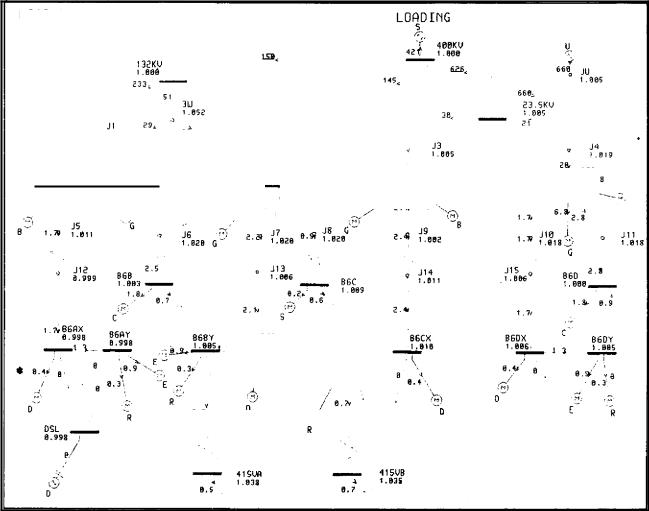
FIG. 2.1 Load flow results for a power station electrical auxiliary system and grid supply system interface connections. The load flows are expressed in terms of MVA loadings with system voltage profile levels in pu values.
of electrical auxiliary systems and associated plant. They involved network reduction techniques, with many design performance approximations and assumptions; sensitivity and iterative studies, invoking permissible system and plant design tolerances, were necessarily of an extremely constrained nature.
With present day computer programs and computing facilities, the analysis techniques are vastly more comprehensive, efficient and precise than older methods. Batch mode and interactive analysis programs enable the predictive performance of station electrical system designs to be optimised on an iterative basis, with much more detail and a higher degree of accuracy than previously, in an extremely short time.
Batch mode computing systems are capable of analysing the performance of more than one power system at a time and are primarily suitable for processing the extensive amounts of information and results associated with the dynamic transient analysis of large systems. Such studies may, for example, involve a computational time of about 10 minutes for a single
short term transient condition of 5 seconds, but they can of course be submitted for analysis during computer off-peak periods at night times and weekends.
Interactive on-line computing, by comparison, allows the design engineer to interface with, and directly control, the analysis process from a computer terminal in respect of the network representation, type of study required, system parameters, corrective actions and output result displays. While interactive computing is highly user orientated and consequently more time demanding at the terminal for the design engineer, it is much faster than batch mode analysis systems in the overall turn round time of producing results, especially for steady state power system studies.
The availability of separate suites of batch mode and interactive computer programs, when coupled with their respective databases, enables a series of specific power system performance or reliability evaluation analysis studies to be undertaken in a uniform manner, by varying the system parameters and the type of study. As a consequence of the ability to control the type
86

Principles of electrical system analysis
' |
1 |
10 |
1.0 |
|
|
0 |
1 |
08 |
|
|
|
|
|
|
|||
|
|
1 05 |
|
|
|
6 - |
|
|
|
|
|
|
|
|
|
|
|
|
1 |
00 |
08 |
|
|
0 9 - |
|
|
1 00 - |
|
|
|
1 |
04 |
|
||
|
|
|
|
||
0 8 - |
1 |
02 |
0 6 |
|
|
4 - |
|
|
0.95 - |
|
|
|
|
|
|
|
|
07 - |
1 00 |
|
|
|
|
3 - |
|
|
0.90 - |
|
|
|
|
|
|
|
|
0.9804
0 6 -
2 " |
096 |
0.85 - |
|
4.01. |
|
|
|
||
|
|
4.111. |
|
|
|
||||
|
|
|
|
|
.11%. |
|
|
|
|
5 — |
|
|
|
|
|
|
|
|
|
|
|
|
|
|
|
|
|
|
|
|
094 |
0.2 |
|
I0 |
|
|
|
.... |
|
|
|
|
|
|
|
|
|
||
s- |
|
0 80 |
|
|
|
|
|
||
1:1 4-- |
0 92 |
|
|
|
|
|
|
|
|
. |
|
|
|
|
|
|
|
||
- 00- |
090 |
00 |
0.75 |
5 |
10 |
15 |
210 |
25 |
|
|
|
|
|
||||||
|
|
|
|
GENERATOR TERMINAL VOLTAGE IPU ON 3.3 kV) |
|
|
|
||
|
|
|
|
■ •• ■P |
GENERATOR OUTPUT POWER (PU ON RATING) |
|
|
|
|
|
|
|
|
|
GENERATOR SPEED (PU ON 50 Hz - 1000 r(min) |
|
|
|
|
|
|
|
|
|
PONY MOTOR SPEED (PU ON 50 Hz H$ OR LS) |
|
|
|
|
|
|
|
|
"-•••••• |
PONY MOTOR CURRENT (PU ON RATING) |
|
|
|
|
FIG. 2.2 Gas circulator pony motor speed change study
of study and sequence of studies from within a suite of programs, the efficiency and speed of response in producing assessments of large complex systems has increased significantly.
For example, having entered all the system and plant data, the design engineer is able to produce the results of a power system steady state analysis or reliability evaluation study within a matter of seconds for a complete power station electrical system, including the grid interface connections. It is also a relatively simple exercise to undertake sensitivity studies to identify the system components and parameters having a critical impact on the overall system performance.
One should not, however, overlook the considerable design effort and time that is involved in setting up the system networks and the collation, checking and entry of the system plant and connection data for modelling and simulating complete station electrical systems fully. This may amount to something in excess of eight man weeks for a large power system.
1.4.1 Reliability evaluation
A reliability evaluation study forms the normal starting point for comparing the effectiveness of alternative
interface connection arrangements between the grid system, the turbine-generator units and the associated station electrical supply systems. The extent of the system evaluation undertaken, using interactive computing programs, incorporates the following analysis features:
•Failure rates.
•Outage durations.
•Outage times.
•Common mode failures.
•Limited energy sources.
•Time dependent reliability.
The basic techniques required to analyse and evaluate the reliability of the systems include the simulation of realistic failure events, restoration procedures, switching actions, maintenance events and operational constraints.
For multiple turbine-generator power stations with identical unit and station systems, it is more efficient to divide the systems into subsystems. This technique, as explained in detail later, is not only efficient and
87

Electrical system analysis |
|
Chapter 2 |
|
|
|
|
|
|
SYSTEM |
|
2 |
|
|
CONSTRUCT A NEW SYSTEM |
SYSTEM |
|||
DRAWING AND |
||||
2 - RETRIEVE A SYSTEM |
RETRIEVAL |
|||
MODIFYING |
|
|||
3 - EXIT FROM THE PROGRAM |
|
ROUTINE |
||
ROUTINE |
|
|||
|
|
|
||
|
|
|
|
|
|
|
|
|
ty |
|
|
|
|
|
||
|
|
|
|
00 YOU WANT TO QUIT PROGRAM Y7N .> |
|
|
|
|
|
|||
|
|
1,4 |
|
|
|
|
|
2 |
|
|
||
|
|
|
|
|
IN |
|
|
|
|
|
|
|
|
|
|
|
|
MAN OPTIONS |
|
|
|
|
|
||
|
|
|
|
- CONSTRUCT A NEW SYSTEM |
|
|
|
|
|
|||
FILING |
3 |
|
2 - RETRIEVE A SYSTEM FROM FILE |
|
|
.4111www...•■■110- |
EDITING |
|||||
|
4 - MODIFY THE PRESENT SYSTEM |
|
|
|||||||||
SYSTEM |
|
3 FILE THE PRESENT SYSTEM DIAGRAM |
|
5 |
DATA |
|||||||
ROUTINE |
|
|
5- EDIT THE PRESENT NETWORK DATA |
|
|
|
ROUTINE |
|||||
|
|
|
|
|
|
|
|
|
||||
|
|
|
|
6 - OUTPUT PROCESS |
|
|
|
|
|
|||
|
|
|
|
7 - EXIT FROM THE PROGRAM |
|
|
|
|
|
|||
|
|
|
|
|
|
|
|
|
|
|
|
|
|
|
|
|
|
|
|
|
|
|
|
|
|
OPTIONS
DISPLAY NETWORK DIAGRAM
DISPLAY FULL LIST OF INPUT DATA
PRINTING OF INPUT DATE
FiG. 2.3 Time dependent reliability analysis program — flow chart
precise but reduces the design engineering effort involved in the preparation and input of system component data.
1.4.2 Power system performance analysis
Batch mode and interactive computing programs are used to assess the performance of integrated and isolated power systems in respect of:
•Load flows, voltage regulation and transformer tapchanger optimisation.
•Short-circuit (symmetrical and asymmetrical) fault levels.
•Dynamic motor starting performance.
•Transient fault stability performance of systems and motors.
•Fast transient switching of systems and motors.
•Transient recovery voltage levels.
•Controller modelling of AVRs, governors and prime movers.
•Power system protection co-ordination of relays and fuses.
Power system performance analysis is largely based on load flow, short-circuit and transient stability studies. The analysis, using nominal plant parameters, commences with the calculation of the steady state power
88

Reliability evaluation of power systems
flows, voltage distributions and short-circuit fault levels throughout the system during no load, minimum load, start-UP and CMR sequence loading (block loading) conditions of the turbine-generator unit operation. During this stage of the analysis, transformer tap changer positions are adjusted, as appropriate, to achieve the optimum system voltage profiles for these conditions of operation. Dynamic motor starting and system transient fault .tability performance evaluation studies are also intro& during this process for the optimisation
of system and plant parameters.
Further stcady state, dynamic response and transient fault stability sensitivity analyses are then performed, selectively invoking permissible plant manufacturing tolerances, defined system operating ranges of voltage and frequency, and credible system and plant outage operating conditions. Calculation of system dynamic responses uses a step-by-step approach, starting from a specified balanced steady state operating condition produced by a load flow study.
Analysis programs contain a number of models for the representation of synchronous machines and induction motors; they automatically select the most suitable model, according to the amount of data provided by the user in terms of the machine model parameters. The most detailed models of a synchronous machine include the transient and sub-transient and saturation function parameters, together with the excitation and speed governor controller model block diagram transfer function elements. Other loads are represented as fixed impedances, while the transformers, transmission and cable connections are represented by their equivalent circuit parameters.
Inclusion of the effects of instantaneous voltage and frequency deviations into the calculations, produces a more realistic assessment of system behaviour under transient conditions. The widely used diesel or gasturbine generator supported essential supply systems in nuclear power stations are examples of such operating situations and a special purpose transient analysis program has been developed for assessing their dynamic performance. This program recalculates the plant and s,stern parameters throughout the transient variations of instantaneous voltage and frequency, thereby enabling the systems and plant to be designed and operated closer to their limits, coupled with the ability to define the settings of the associated protective devices more accurately.
Detailed descriptions of power system reliability ev aluation and performance analysis are given in the following Sections 2 and 3 respectively. These descriptions are comprehensively illustrated by authentic computer printouts generated by the software programs under discussion, i.e., they have not been subjected to any form of artistic licence.
1.5 Quality assurance of analysis programs
Particular emphasis is placed on achieving the highest
possible standard of quality by instituting rigorous verification and validation testing disciplines from the inception of a program up to the stage when it is formally released in a production status version. Test systems, representative of the wide spectrum of the electrical systems encountered within power stations, are used for the quality assurance of all program versions and enhancements.
Each development and production version of a program is identified with a unique identification reference, which is displayed on the VDU during analysis and is subsequently printed automatically on the system input, network diagrams, graphical and output data sheets.
At an early period in the development process, an appropriate level of verification and validation testing is initiated and formally recorded with respect to program source codes, models, calculations and control routines. Verification activities are progressively increased during the development, involving extensive testing and comparison of the source codes with the mathematical models by the specialist software programmer.
The verification and validation tasks are the responsibility of the design engineer, who undertakes a comprehensive comparison of the mathematical models and program results with manual calculations, field measurements of plant and system performance tests and, whenever applicable, with earlier versions of the program and alternative validated analysis programs. The widespread utilisation of a program by many design engineers for the analysis of various types of integrated and isolated power systems is an additional i mportant contribution to the verification and validation process.
Notwithstanding the procedures and disciplines outlined it is recognised that the verification, validation and modification of computer programs may continue for many years following their formal introduction at a production status level. Rigid quality control disciplines must continue to be exercised in this regard in accordance with the procedures outlined.
2 Reliability evaluation of power systems
2.1 Introduction
The reliability of larger turbine-generator units (500 MW and above) in modern power stations is assuming increasing significance in terms of system security and the economics of supply, since they are used in the main to meet the base load requirements of the grid system.
It follows that all the supporting auxiliary plant and systems within each station must have a similar high degree of reliability, in order to minimise the impact of their failure on the overall reliability of the main units.
89
Electrical system analysis |
Chapter 2 |
|
|
The Station Electrical System (SES) is an example of one such internal system: it can be considered to have three constituent parts:
•The MAIN system, the principal function of which is to distribute a sufficient supply of electrical power of the required quality to all the drives and auxiliary plant associated with the boilers/reactors and turbine-generators. Failure of all or even part of this system could have a direct impact on the availability of a main generator, causing either the total loss or reduction of output from the generator to the grid system.
•The GUARANTEED system which supplies power of guaranteed quality to computers, instruments, etc., necessary for the operational control and monitoring of the power station. Sometimes this is referred to as the No-break system and is required to continue to function during large system disturbances, unit start, shutdown, etc.
•The ESSENTIAL system which comprises standby generators and associated electrical connections and drives (some of which are common with the MAIN system). This is sometimes called the Short-break system and is generally used (with or without the standby generators) to supply power to all those auxiliaries necessary for the safe operation and posttrip cooling requirements of nuclear stations and for black starting of fossil-fired stations.
It is important, therefore, that a reliability assessment of all three parts of the SES is performed during, and as an integral part of, the design process and should cover all the system operating configurations and station running modes.
Reliability assessment, as such, is not a new requirement. Engineers have always striven to design systems that will continue to operate in a safe and reliable manner. In the past, this reliability has generally been achieved by drawing on the experience of design and operational staff and using purely engineering and qualitative criteria. Quantitative assessment, due mainly to the sheer tedium of the calculations involved, tended to be limited to the evaluation of relatively small systems (comprised of few components).
2.2 Quantitative reliability evaluation
It is clear that a quantitative evaluation of the SES reliability is of considerable help in decision making during the design phases of any power station project. It consists of the calculation of a set of numerical indices which provides a measure of the 'goodness' of the system and can be used during the design phase to compare one system with another.
2.2.1 Choice of numerical indices
There are many reliability indices that could be cal-
culated and used as a measure of the 'goodness' of a SES. The following are typical examples of suitable indices:
FR |
Failure Rate, the expected average |
|
number of failures in a specified period |
MTBF |
The Mean Time Between Failures |
MTTR |
The Mean Time To Repair |
AOD |
The Average Outage Duration or average |
|
down time |
OT or OD The total Outage Time or total Outage Downtime in a specified period
LOG |
The total Loss Of Generation in a spe- |
|
cified period due to system unreliability |
LOR |
The total Loss Of Revenue in a specified |
|
period due to system unreliability |
ER |
The Encounter Rate for operation in |
|
various derated states (see (b) below). |
The interactive computer programs developed specifically for the quantitative reliability evaluation of power station electrical systems (described in Section 2.3 of this chapter) calculate, list and/or display the reliability indices. The following indices have been selected as the most useful and appropriate in the iterative process of system design:
(a)For a particular load point or node of a SES:
F R Expected average number of failures of supply to the load point in a year (failures/year)
AOD Average outage duration or downtime — average time for which no supply is available at the load point (hours)
AOT Total annual outage time — total time in a year when no supply is available at the load point — (hours/year).
(b)For the SES as a whole:
ER |
Expected frequency of operation of the |
|
power station or main generator unit in |
|
various derated states in a year (occasions/ |
|
year) |
AD |
Average duration of operation in each of |
|
the derated states (hours) |
AOT Total time of operation in each of the derated states in a year (hours/year)
LOG Expected loss of generation in a year due to the unreliability of the SES (MWh/year).
2.2.2 Scope of reliability evaluation assessments
The availability of very powerful modern mainframe computers led to the development of efficient computer
90
|
|
|
Reliability evaluation of power systems |
|
|
|
|
||
|
programs containing algorithms which facilitate the |
2.3.1 Batch program — RELAPSE |
||
|
probabilistic assessment of the reliability of very large |
During the first development project, the techniques, |
||
|
electrical systems (systems containing a very large num- |
|||
|
which are described in more detail in Section 2.5 of |
|||
|
ber of components). With such computing facilities, |
|||
|
this chapter, were incorporated into a computer pro- |
|||
|
the system design engineer is provided with a very |
|||
|
gram designed to run in batch mode but capable of |
|||
|
powerful design aid. |
|||
|
analysing only small systems (containing up to about |
|||
|
|
Such assessments facilitate the following design |
15 load point busbars or nodes). |
|
|
|
|
||
|
activities: |
This first batch program (called RELAPSE — |
||
|
• |
The corn larison of alternative designs of SES with |
Reliability Evaluation of Electrical Systems) was not |
|
|
very 'user friendly'. The data preparation stage was |
|||
|
|
regard to the reliability of supply to corresponding |
||
|
|
extremely laborious, requiring the completion of nu- |
||
|
|
nodes or 1 aad point busbars in each system to which |
||
|
|
merous data sheets from which sets of punched cards |
||
|
|
it is proposed to connect certain critical plant. |
||
|
|
were produced. It was necessary for these to be checked |
||
|
|
|
||
|
• |
Indication of how a system may fail, assessing the |
thoroughly for accuracy and arranged in the correct |
|
|
|
consequences of such failures and providing suffi- |
order in a deck suitable for computer input via a card |
|
|
|
cient information to enable the quality of a system |
reader. The turnaround for each study took anything |
|
|
|
to be related to agreed reliability standards or tar- |
up to three days. |
|
|
|
gets. Where the agreed standards/targets are not |
|
|
|
|
achieved, sensitivity calculations can be undertaken |
2.3.2 interactive program — GRASP (Version 1) |
|
|
|
during the design phase to enable the design engineer |
||
|
|
The main objective of the next development project |
||
|
|
to decide what improvements to the system should |
||
|
|
was an interactive version of the RELAPSE program, |
||
|
|
be made and whether the capital cost of such im- |
||
|
|
suitable for running under a time sharing system (TSO) |
||
|
|
provements (if any) is acceptable. |
||
|
|
from a remote graphics terminal. Briefly, this work |
||
|
|
Quantitative assessments of the loss of generation |
||
|
• |
entailed the improvement of the RELAPSE algorithms |
||
|
|
(in MWh/year) resulting from the unreliability of |
to make them more efficient and the development of |
|
|
|
the SES. The unreliability of the SES can thus be |
new algorithms for the graphics drawing routines, |
|
|
|
expressed in financial terms by applying the current |
data entry and editing, file storing and retrieval, etc., |
|
|
|
figure for the marginal cost of replacement genera- |
all of which were designed to make the program more |
|
|
|
tion (running alternative plant which is more ex- |
'user friendly'. |
|
|
|
pensive in terms of cost per unit output). |
With this interactive program (called GRASP — |
|
|
• Checking that, for a nuclear station, the proposals |
Graphic/interactive Reliability of Auxiliary Systems |
||
|
of Power stations), once having set up the system to |
|||
|
|
for the provision of local (on-site) standby generation |
be evaluated and entered the appropriate data, full |
|
|
|
and the methods of connecting this to the SES, |
'on-the-spot' control of the analysis study is available |
|
|
|
ensures that the contribution of the SES to the total |
to the user. Not only can the basic assessment of the |
|
|
|
probability of a degraded core does not exceed the |
system be undertaken but, due to the flexibility built |
|
|
|
agreed design target. |
into the program, a whole range of sensitivity studies |
|
• Inclusion of the effects of common mode failure |
can very easily and quickly be undertaken by changing |
|||
the system topology and/or data and re-running the |
||||
|
|
(CM F) in an assessment of the SES (if suitable data |
||
|
|
study to obtain instant results. Various options are |
||
|
|
is available) when the proposed physical disposition |
||
|
|
built into the program, which can be exercised by the |
||
|
|
of the various components is known. Alternative- |
||
|
|
user to control both the precision and objectives of |
||
|
|
ly (even without such CMF data), the sensitivity |
each study. |
|
|
|
of the system reliability indices to the CMF of cer- |
Part of this development also included increasing |
|
|
|
tain groups or sets of system components can be |
the array dimensions within the program to enable |
|
|
|
examined. |
much larger systems (containing up to about 50 nodes) |
|
|
|
|
||
|
|
|
to be evaluated and inserting full protection against |
|
2.3 Computer programs for reliability |
malfunctioning of the program, together with appro- |
|||
priate error message displays. |
||||
evaluation |
The interactive drawing routines developed for the |
|||
The CEGB has undertaken, over many years, the |
GRASP program are very similar (as perceived by the |
|||
user) to those of the Interactive Power Systems A nalysis |
||||
de‘,.elopment of computer analysis programs specifi- |
||||
cally for power system reliability evaluation, by adapt- |
(IPSA) programs described elsewhere in this chapter. |
|||
|
||||
ing and enhancing any techniques that can be applied |
2.3.3 Interactive program — GRASP (Version 2) |
|||
to the numerical evaluation of reliability and incor- |
||||
|
||||
porating these techniques in computer programs for |
During the development and use of GRASP1, it |
|||
use in system design. |
was recognised that the scope and efficiency of re- |
|||
|
|
|
||
91
Electrical system analysis |
Chapter 2 |
|
|
liability assessments could be significantly enhanced by the introduction of subsystem concepts, common mode failure evaluation and limited energy sources representation.
Subsystem concepts'
Due to the fact that, for a reliability evaluation, the graphical input of a system had to be performed on a component-by-component basis, it became apparent that this was now the most tedious part of the work required of the user of the interactive program.
Recognising that, in general, the SES for a typical power station could be broken down into four or five broadly similar subsystems, the next development project included (amongst other things) the provision of an improved graphics drawing system. The system developed is known as the Subsystem Drawing Routine.
With this system, implemented in the GRASP2 interactive computer program, it is only necessary to input the system and data for, say, the SES associated with one generator unit of a four-unit station and then use the computer to reproduce this three times and store as separate subsystems. It is possible, of course, to retrieve each of the individual subsystems and make minor changes in the normal way. For a complete representation and subsequent analysis of the complete SES for a four-unit station, it is then necessary to draw the remainder of the SES, i.e., the Station System, separately as the fifth subsystem and use the Interconnector Drawing Facility to interconnect all five subsystems, as necessary.
The result of this development is to reduce to about one-third, the effort required of the user to input a large system, compared with that previously required with GRASP I.
Common mode failure evaluation
The batch computer program RELAPSE and the first interactive program GRASP I only included overlapping independent failure events and maintenance events.
It is a requirement in laying out a power station that segregation is maintained between the components of each power system, and those of all other systems. This is not easily achievable due to space limitations, and can be very costly. The close proximity of components, such as can occur within cable tunnels, switchrooms, etc., suggests that certain groups of components are susceptible to common mode failure.
To add more precision to the assessment of the reliability of a SES, this development included the extension of the algorithms, drawing routines and models and equations within the GRASP2 interactive program, so that events involving the common mode failure of certain user specified groups/sets of components could be included in the evaluation.
Limited energy sources
Although the techniques developed and incorporated within the RELAPSE and GRASP I programs included restoration modes which made use of local standby generators, no account was taken of the fact that such standby plant may only be capable of supplying the required system power for a limited time. Under circumstances where, for example, a time limit was imposed by the size of on-site fuel storage tanks, the assessment of the SES reliability would not be correct, if the restoration mode involved the use of the standby plant.
New algorithms were therefore developed for the GRASP2 program to take account of this time limit and thereby permit a more realistic representation and assessment of the real system.
2.4 Data requirements
The methods of reliability evaluation used within the GRASP interactive computer programs require a selection of the following component reliability data, according to the purpose and wider objectives of each study.
2.4.1 Active failure rate
The average number of times per year that a component fails actively.
A component active failure is defined as one which results in the operation of protective devices to isolate the entire zone around the failed component automatically, e.g., a short-circuit.
2.4.2 Passive failure rate
The average number of times per year (failures/year) that a component fails passively.
A component passive failure is defined as one which does not result in the operation of any protective device but would nevertheless cause loss of supply to the busbar under consideration, e.g., an open-circuit or the false opening of a circuit-breaker.
2.4.3 Total failure rate
The average of the total number of failures per year (for which records are available) that require the removal of the component from service for repair due to either of its failure modes (active and passive).
2.4.4 Average repair time
The average time (hours/failure) taken to repair all failures (active and passive), for each component.
2.4.5 Switching time
Following a component active failure, the average ti me (hours) taken to isolate manually the failed com-
92