

plc advanced functions - 16.22
16.5 DESIGN TECHNIQUES
16.5.1 State Diagrams
The block logic method was introduced in chapter 8 to implement state diagrams using MCR blocks. A better implementation of this method is possible using subroutines in program files. The ladder logic for each state will be put in separate subroutines.
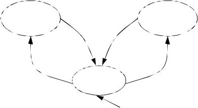
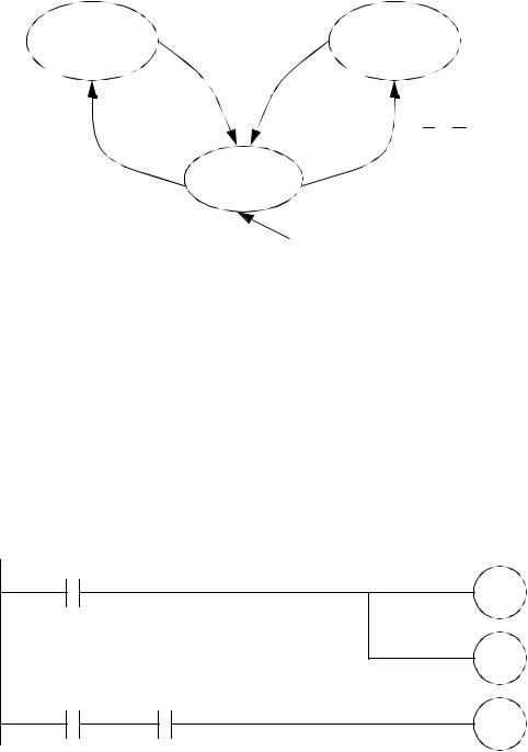
Consider the state diagram in Figure 16.23. This state diagram shows three states with four transitions. There is a potential conflict between transitions A and C.
STA |
STC |
B |
D |
A |
C |
|
STB |
|
first scan |
Figure 16.23 A State Diagram |
|
O:000/00 = STA O:000/01 = STB O:000/02 = STC
The main program for the state diagram is shown in Figure 16.24. This program is stored in program file 2 so that it is run by default. The first rung in the program resets the states so that the first scan state is on, while the other states are turned off. Each state in the diagram is given a value in bit memory, so STA=B3/0, STB=B3/1 and STC=B3/2. The following logic will call the subroutine for each state. The logic that uses the current state is placed in the main program. It is also possible to put this logic in the state subroutines.
plc advanced functions - 16.23
S2:1/15 - first scan
L B3/1 - STB
U B3/0 - STA
U B3/2 - STC
B3/0 - STA
JSR program 3
B3/1 - STB
JSR program 4
B3/2 - STC
JSR program 5
B3/0 - STA
L O:000/0
B3/1 - STB
L O:000/1
B3/2 - STC
L O:000/2
Figure 16.24 The Main Program for the State Diagram (Program File 2)
The ladder logic for each of the state subroutines is shown in Figure 16.25. These blocks of logic examine the transitions and change states as required. Note that state STB includes logic to give state C higher priority, by blocking A when C is active.
plc advanced functions - 16.24
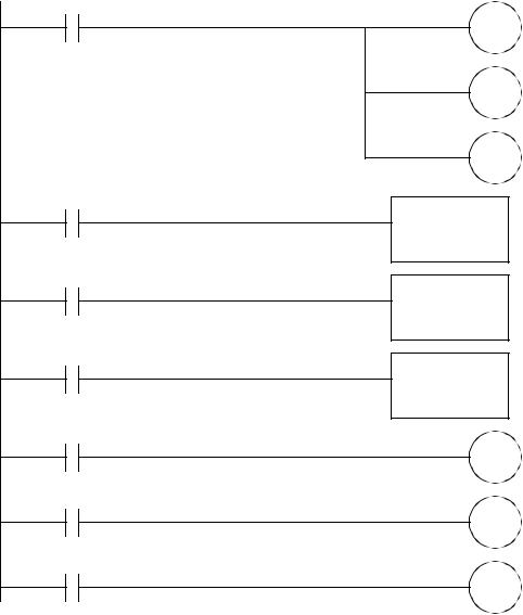
Program 3 for STA
B
U B3/0 - STA
L B3/1 - STB
Program 4 for STB
C
U B3/1 - STB
L B3/2 - STC
A C
U B3/1 - STB
L B3/0 - STA
Program 5 for STC
D
U B3/2 - STC
L B3/1 - STB
Figure 16.25 Subroutines for the States
The arrangement of the subroutines in Figure 16.24 and Figure 16.25 could experience problems with racing conditions. For example, if STA is active, and both B and C are true at the same time the main program would jump to subroutine 3 where STB would be turned on. then the main program would jump to subroutine 4 where STC would be turned on. For the output logic STB would never have been on. If this problem might occur, the state diagram can be modified to slow down these race conditions. Figure 16.26 shows a technique that blocks race conditions by blocking a transition out of a state until the transition into a state is finished. The solution may not always be appropriate.
plc advanced functions - 16.25
STA |
|
|
|
|
|
STC |
|
|
|
|
D*C |
||||
B*A |
|||||||
|
|
||||||
|
|
|
|
||||
|
|
|
|
|
C*(B + D) |
|
A*(B + D) |
||||||
|
||||||
|
|
|
|
|
STB |
|
first scan
Figure 16.26 A Modified State Diagram to Prevent Racing
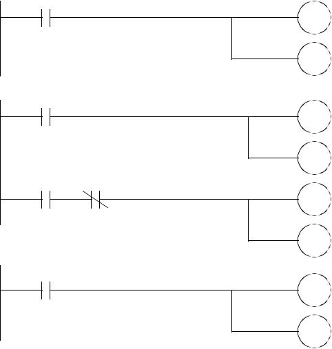
Another solution is to force the transition to wait for one scan as shown in Figure 16.27 for state STA. A wait bit is used to indicate when a delay of at least one scan has occurred since the transition out of the state B became true. The wait bit is set by having the exit transition B true. The B3/0-STA will turn off the wait B3/10-wait when the transition to state B3/1-STB has occurred. If the wait was not turned off, it would still be on the next time we return to this state.
Program 3 for STA
B3/10 - wait
U B3/0 - STA
L B3/1 - STB
B B3/0 - STA
B3/10 - wait
Figure 16.27 Subroutines for State STA to Prevent Racing