

continuous sensors - 23.32
23.2.9 Others
A number of other detectors/sensors are listed below,
Combustion - gases such as CO2 can be an indicator of combustion
Humidity - normally in gases
Dew Point - to determine when condensation will form
23.3 INPUT ISSUES
Signals from sensors are often not in a form that can be directly input to a controller. In these cases it may be necessary to buy or build signal conditioners. Normally, a signal conditioner is an amplifier, but it may also include noise filters, and circuitry to convert from current to voltage. This section will discuss the electrical and electronic interfaces between sensors and controllers.
Analog signal are prone to electrical noise problems. This is often caused by electromagnetic fields on the factory floor inducing currents in exposed conductors. Some of the techniques for dealing with electrical noise include;
twisted pairs - the wires are twisted to reduce the noise induced by magnetic fields. shielding - shielding is used to reduce the effects of electromagnetic interference. single/double ended inputs - shared or isolated reference voltages (commons).
When a signal is transmitted through a wire, it must return along another path. If the wires have an area between them the magnetic flux enclosed in the loop can induce current flow and voltages. If the wires are twisted, a few times per inch, then the amount of noise induced is reduced. This technique is common in signal wires and network cables.
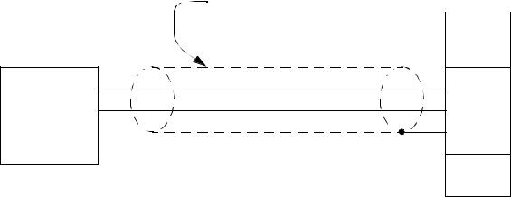
A shielded cable has a metal sheath, as shown in Figure 23.32. This sheath needs to be connected to the measuring device to allow induced currents to be passed to ground. This prevents electromagnetic waves to induce voltages in the signal wires.
Analog voltage source
+
-
continuous sensors - 23.33
A Shield is a metal sheath that |
Analog Input |
|
surrounds the wires |
|
|
|
|
|
IN1
REF1
SHLD
Figure 23.32 Cable Shielding
When connecting analog voltage sources to a controller the common, or reference voltage can be connected different ways, as shown in Figure 23.33. The least expensive method uses one shared common for all analog signals, this is called single ended. The more accurate method is to use separate commons for each signal, this is called double ended. Most analog input cards allow a choice between one or the other. But, when double ended inputs are used the number of available inputs is halved. Most analog output cards are double ended.

device +
#1 -
device +
#1 -
continuous sensors - 23.34
|
|
|
|
device |
+ |
|
|
|
|
Ain 0 |
|
|
|
||
|
|
|
|
|
|||
|
|
|
#1 |
- |
|
|
|
|
|
|
|
|
|
||
|
|
Ain 1 |
|
|
|
|
|
|
|
|
|
|
|
|
|
|
|
|
|
device |
+ |
|
|
|
|
Ain 2 |
|
|
|||
|
|
|
|
|
|||
|
|
|
#1 |
- |
|
|
|
|
|
|
|
|
|
||
|
|
Ain 3 |
|
|
|
|
|
|
|
|
|
|
|
|
|
|
|
|
|
|
|
|
|
|
|
Ain 4 |
|
|
|
|
|
|
|
|
|
|
|
|
|
|
|
Ain 5 |
|
|
|
|
|
|
|
|
|
|
|
|
|
|
|
Ain 6 |
|
|
|
|
|
|
|
|
|
|
|
|
|
|
|
Ain 7 |
|
|
|
|
|
|
|
|
|
|
|
|
|
|
|
COM |
|
|
|
|
|
|
|
|
|
|
|
|
|
|
|
|
|
|
|
|
|
Ain 0
Ain 0
Ain 1
Ain 1
Ain 2
Ain 2
Ain 3
Ain 3
Single ended - with this arrangement the signal quality can be poorer, but more inputs are available.
Double ended - with this arrangement the signal quality can be better, but fewer inputs are available.
Figure 23.33 Single and Double Ended Inputs
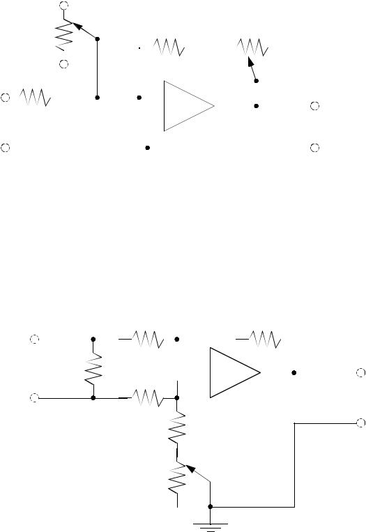
Signals from transducers are typically too small to be read by a normal analog input card. Amplifiers are used to increase the magnitude of these signals. An example of a single ended signal amplifier is shown in Figure 23.34. The amplifier is in an inverting configuration, so the output will have an opposite sign from the input. Adjustments are provided for gain and offset adjustments.
Note: op-amps are used in this section to implement the amplifiers because they are inexpensive, common, and well suited to simple design and construction projects.
When purchasing a commercial signal conditioner, the circuitry will be more complex, and include other circuitry for other factors such as temperature compensation.
continuous sensors - 23.35
+V |
|
|
|
|
|
|
|
|
|
|
|
|
|
|
|
|
|
|
Ro |
offset |
|
Rf |
|
|
|
Rg |
|||||||||||
|
|
|
|
|
|
|
|
|
|
|
|
|
|
|
|
|
||
|
|
|
|
|
|
|
|
|
|
|
|
|
|
|
|
|
|
|
-V |
|
|
|
|
|
|
|
|
|
- |
|
|
|
gain |
||||
|
|
|
|
|
|
|
|
|
||||||||||
|
|
|
|
|
|
|
|
|
|
|
|
|
|
|
|
|
|
|
|
|
|
|
|
|
|
|
|
|
|
|
|
|
|
|
|
|
|
|
|
|
|
|
|
|
|
|
|
|
|
|
|
|
|
|
||
Ri |
|
|
|
|
|
|
|
|
|
+ |
|
|
|
|
|
|
|
|
|
|
|
|
|
|
|
|
|
|
|
|
|
Vout |
|||||
|
|
|
|
|
|
|
|
|
|
|
|
|
|
|
||||
Vin |
|
|
|
|
|
|
|
|
|
|
|
|
|
|
|
|||
|
|
|
|
|
|
|
|
|
|
|
|
|
|
|
|
|
|
|
|
|
|
|
|
|
|
|
|
|
|
|
|
|
|
|
|
|
|
|
|
|
|
|
|
|
|
|
|
|
|
|
|
|
|
|
|
|
|
|
|
|
|
|
|
|
|
|
|
|
|
|
|
|
|
|
|
Vout = |
Rf |
+ Rg |
+ offset |
----------------- Vin |
|||
|
|
Ri |
|
Figure 23.34 A Single Ended Signal Amplifier
A differential amplifier with a current input is shown in Figure 23.35. Note that Rc converts a current to a voltage. The voltage is then amplified to a larger voltage.
|
|
|
R1 |
|
|
- |
Rf |
|
|
|
Iin |
Rc |
|
|
|
|
|
||||
|
|
|
|
|||||||
+ |
|
|
|
|
||||||
|
R2 |
|
|
|
|
|||||
|
|
|
|
|
|
|
||||
|
|
|
|
|
|
|
|
|
||
Vout
R3
R4
Figure 23.35 A Current Amplifier
continuous sensors - 23.36
The circuit in Figure 23.36 will convert a differential (double ended) signal to a single ended signal. The two input op-amps are used as unity gain followers, to create a high input impedance. The following amplifier amplifies the voltage difference.
-
+
Vin |
|
|
- |
|
|
||||
|
+ |
|||
|
||||
|
|
|||
|
|
|
|
|
Vout
-
+
CMRR adjust
Figure 23.36 A Differential Input to Single Ended Output Amplifier
The Wheatstone bridge can be used to convert a resistance to a voltage output, as shown in Figure 23.37. If the resistor values are all made the same (and close to the value of R3) then the equation can be simplified.