Экзамен зачет учебный год 2023 / Stoter, 3D Cadastre

9.5. Generalisation of the integrated TIN

(a)

(b)

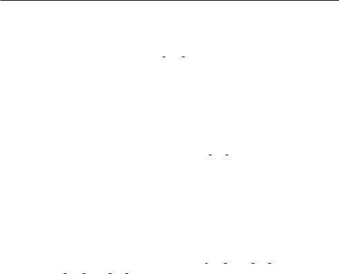
Figure 9.11: Conforming TIN in which point heights and 2D planar partition of parcels are integrated, before (above) and after (below) filtering.

should participate in the generalisation. Therefore the integrated height and object model could be further generalised by taking into account both the elevation aspect and the 2D objects at the same time. It is already possible to separate generalisation of the terrain model [14, 18, 88, 164] and 2D objects [33, 134, 141, 166, 177, 192, 235]. However, the integrated generalisation of the height and object model makes this model also well suitable for other resolutions (scales) or even in a multi-resolution context.

Starting with the detailed-to-coarse approach one could identify the following steps:

Step 0: Integrate raw elevation model (AHN) and objects (parcel boundaries) in a (conforming or refined constrained) TIN, see section 9.3.

205

Chapter 9. Integrating 2D parcels and 3D objects in one environment

Step 1: Improve the e ciency of the TIN created in step 0 by removing AHN points from the TIN until this is not longer possible given the maximum tolerance value in the vertical direction: eps vert 1 (as described in section 9.5.1). Note that this tolerance could be adjusted for di erent circumstances, but the initial value should be the same size as the accuracy of the input data.

Step 2: Now also start generalisation of the object boundaries, for example with the Douglas-Peucker line generalisation algorithm, by removing those boundary points which do not contribute significantly to the shape of the boundary. This can be done in 2D (standard Douglas-Peucker), but it is better to apply this algorithm in 3D. Keep on removing points until this is impossible within the given tolerance in the horizontal direction: eps hor 1. After this line generalisation of the constraints, re-triangulate the TIN according to the rules as in step 0 (of a conforming or refined constrained TIN).

Step 3: Finally, for multi-resolution purposes, also start aggregating the objects, for example in our case: parcels to sections (and the next aggregation level would be sections to municipalities, followed by municipalities to provinces, etc.). In fact this is removing some of the constrained edges (original parcel boundaries) from the input of the integrated model. Repeat step 1 and 2 with other values for the epsilon tolerances at every aggregation level with their own tolerances in the vertical and horizontal direction: eps vert 2, eps hor 2 (at the section level), eps vert 3, eps hor 3 (at the municipality level), ....

9.6Generalisation prototype

The first steps (step 0 and step 1) of the generalisation method have been implemented in a prototype. The fundamental idea of the implemented filtering method is to detect characteristic points (detailed-to-coarse approach). Points that are not characteristic, i.e. they do not contribute significantly to the height surface, will be removed. The question whether points are characteristic, is in the prototype dependent on the following conditions:

•A point is characteristic if the slope of two neighbouring triangles of the point are significantly di erent [18]. To detect this, the normal vectors for the neighbouring triangles are determined and compared. If the di erence is bigger than a given threshold angle, the point will be defined as characteristic and not be removed from the TIN.

•Local minima and maxima are also characteristic points of a TIN. If two neighbouring triangles are in the same direction in the first condition, the change in angle is less important than where the change in angle demarcates a top or a valley. Therefore, a smaller threshold angle is used when the specific point is a local minimum or maximum. A minimum or maximum is the case when the azimuths of the slope of two neighbouring triangles are opposite of each other, which can be determined by calculating the di erences in the azimuths. If the di erence is bigger than a given threshold value, a smaller threshold angle is used in the first condition.

206

9.6. Generalisation prototype

Based on these conditions a point is maintained or removed. If two neighbouring triangles of one point already fulfil one of the criteria, the point will be maintained. The next step is to look if the removal of a point can be justified. This test is done by calculating the height di erence at the location of the removed point between the original TIN and the new TIN (which is generated based on the reduced data set). If this di erence is bigger than a threshold value the removed point is re-added. After this step the data reduction is performed again, i.e. the data reduction is an iterative process until the process is stopped on user request, preferably when a more or less stable data set is obtained (e.g. when all points have been found to be characteristic).

The prototype has been implemented in the 3D Analyst extension of ArcView (ESRI) using the macro language of ArcView (avenue). In ArcView the TIN is recognised as an object and therefore the TIN data structure can be used directly in the reduction algorithm and in addition the results can easily be visualised. This prototype shows already the possibility of data reduction on a TIN, but should be implemented as part of the database in the future, once a TIN data structure is supported as data type in a geo-DBMS.

For our initial test, the data reduction is performed on the unconstrained TIN. This means that the 2D objects and the point heights are kept separately during the data reduction process in order to get a first impression of the achievable results. Incorporating the constraints at this stage would have made the data reduction process more complex. Figure 9.11 shows the conforming TIN of our test data set, after filtering. We did experiments with di erent parameters. The parameters that showed best results were:

•minimum angle between two neighbouring triangles to be a characteristic point if a point is not a top or a valley: 4.5 degrees;

•minimum angle between two neighbouring triangles to be a characteristic point in case of a top or valley: 3 degrees;

•di erence in azimuth between two neighbouring triangles to determine if two triangles are opposite of each other: 120 degrees;

•maximum allowed di erence in height to determine if a removed point should be re-added: 0.25 meters.

Apart from the minimum angle, the chosen parameters are based on previous research [167].

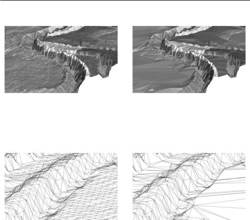
The data set used in this example covers an area of 1450 by 800 meters and contains 44,279 AHN points (maximum z-value 14.2 meters, minimum z-value 6.7 meters, mean 9.5 meters). Three iterations steps were used to filter the data set. Figures 9.12 and 9.13 clearly illustrate how the filtering maintains all terrain shapes but reduced the number of points substantially (height is exaggerated ten times).

In the first iterative step, 34,457 AHN points were removed (9,822 were considered to be characteristic). The average height di erence between the original and the new TIN was 0.09 meter. 3,243 points were re-added since they exceeded the height di erence of 0.25 meter, which resulted in 13,065 points after the first step. After the second iteration step 8,697 points were determined as characteristic, the average height di erence between the new and the original point was again 0.09 meter, 3,469

207

Chapter 9. Integrating 2D parcels and 3D objects in one environment

Figure 9.12: Detail of filtering results: before (left) and after (right) data reduction.

Figure 9.13: Detail of filtering results: before (left) and after (right) data reduction.

points were re-added and this all resulted in 12,166 points. After the third iteration step, 8,455 points were considered to be characteristic (average height di erence 0.09 meter) and 3,529 points were re-added. After this step the data reduction process was stopped. The results of the data reduction process are listed in the following table:

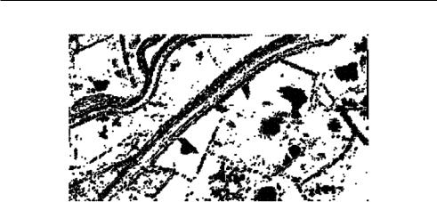
After the total data reduction process 11,984 points from the original 44,279 points were maintained. This is a reduction of 73%. As can be seen from figure 9.14, points were removed from areas with little height variance, while density of point heights in areas with high height variance (e.g. on the dikes) is still high.

The experiments with the prototype on the selected data set yielded a number of conclusions. The minimum angle needs to be adjusted to characteristics of the terrain:

208

9.7. Conclusions

Figure 9.14: Result of data set after data reduction (points not removed are black).

in case of many points in relative flat area, the minimum angles needs to be small in order to avoid clusters of removed points being re-added since they exceed the maximum allowed height di erence. A small minimum angle avoids removing at least one of the points in the cluster. In this case the new TIN is more equal to the original TIN, therefore removed points do not exceed the maximum height di erence condition and they are not re-added. In terrain with more height variance, larger minimum angles are needed in order to remove more points. In mixed terrain (with both areas with low height variance and areas with high height variance, which will often be the case), a balance should be found. In the future one could think of an implementation that can di er the parameters during one data reduction process based on the local height variance.

9.7Conclusions

A basic aspect of a 3D cadastre is to combine 3D objects with parcels in the DBMS. This combination makes it possible to indicate where a 3D object is located with respect to the surface level (what is the depth/height of a 3D object at this location?) and with respect to parcels on the surface.

It was concluded that defining 3D objects with absolute z-coordinates (instead of using z-coordinates with respect to the surface) is the most sustainable way of defining 3D objects. Using absolute values for 3D objects, height surfaces of parcels are needed to be able to combine the parcels and the 3D objects.

Incorporating the planar partition of 2D objects, e.g. the cadastral map, into a height surface makes it possible to extract the 2.5D surfaces of 2D objects and to visualise 2D maps in a 3D environment by using 2.5D representations.

As described and discussed in section 9.3 it is not easy and straightforward to create a good integrated elevation and object model. Several alternatives were investigated, unconstrained Delaunay TIN, constrained TIN, conforming TIN, and finally refined

209

Chapter 9. Integrating 2D parcels and 3D objects in one environment

constrained TIN. After some analyses, the most promising solution, the refined constrained TIN, was selected and applied with success to our test case with real world data: AHN height points and parcel boundaries.

The integrated model however, contains too many AHN points, which do not contribute much to the actual terrain description. Therefore we proposed a method to generalise the integrated model. This method takes both the elevation aspect and the 2D objects into account at the same time. We implemented the first step of this method into a prototype. In this prototype non-characteristic points are removed from the (unconstrained) TIN in an iterative generalisation process. As can be concluded from experiments with the prototype, it is possible to determine important terrain characteristics by using a simple criterion (di erence in angle of neighbouring triangles). With this method it is possible to reduce the data set considerably. The test data contained about 4 times less points after filtering, but still within the epsilon tolerance of the same size as the quality of the original input data sets. On the other hand significant information on the height surface is still available in the TIN. The initial filtering yielded therefore a much-improved integrated model. Improvements can be expected when removed points are not re-added collectively but one-by-one or when the used parameters can di er during one data reduction process, based on local terrain characteristics.

The integrated model is a good basis to obtain a 2.5D representation of 2D parcels (2D parcels draped over a height surface). This is required when combining 3D objects and 2D parcels in one environment.

210

Part III

Models for a 3D cadastre

211

Chapter 10

Conceptual model for a 3D cadastre1

In the previous chapters the need for a 3D cadastre and the conceptual and technical framework for modelling 2D and 3D situations were studied. These chapters sketched the juridical, cadastral and technical frameworks where a 3D cadastre, to some extent, should fit in.

Based on the theory and findings in the previous chapters, this chapter will come to a design of a conceptual schema for a 3D cadastre. Three possible concepts (with several alternatives) have been distinguished to register 3D situations. These three concepts will be introduced in section 10.1. The three conceptual models for 3D cadastral registration with their alternatives are further completed in sections 10.2 to 10.4.

The solutions proposed in this chapter are considered both using (Dutch) cadastral criteria and technological criteria in section 10.5. Based on these considerations the best concepts for 3D registration are selected.

The chapter ends with conclusions.

10.1Introduction of possible solutions

The term ‘3D cadastre’ can be interpreted in many ways ranging from a full 3D cadastre supporting volume parcels, to the current cadastre in which limited information is maintained on 3D situations. Here three fundamental concepts are distinguished (with several alternatives): the most advanced solution, the most simple solution and one in between in which 3D situations are still registered within the current cadastral and technical framework:

• Full 3D cadastre:

1Part of this chapter is based on [202].

213

Chapter 10. Conceptual model for a 3D cadastre

–Alternative 1: combination of infinite parcel columns and volume parcels, (i.e. combined 2D/3D alternative)

–Alternative 2: only parcels are supported that are bounded in three dimensions (volume parcels)

•Hybrid cadastre:

–Alternative 1: registration of 2D parcels in all cases of real property registration and additional registration of 3D legal space in the case of 3D property units

–Alternative 2: registration of 2D parcels in all cases of real property registration and additional registration of physical objects

•3D tags linked to parcels in current cadastral registration

1.A full 3D cadastre

This means introduction of the concept of (property) rights in 3D space. The 3D space (universe) is subdivided into volume parcels partitioning the 3D space. The legal basis, real estate transaction protocols and the cadastral registration should support the establishment and conveyance of 3D rights. The 2D cadastral map does not lay down any restrictions on 3D rights, i.e. rights that entitle persons to volumes are not related to the surface configuration. Rights and restrictions are explicitly related to volumes. Apartment units will be real estate objects defined in 3D, on which a subject can have a right in rem. The full 3D cadastre requires a change in the juridical way of thinking as well as in the cadastral and technical framework. For a full 3D cadastre, the same UML model as described in section 2.2 applies. However, the real estate object may now also be defined in 3D. Two alternatives are distinguished for the full 3D cadastre. In the first alternative volume parcels (bounded parcels) are only established in 3D situations and therefore it is still possible to establish parcels that are defined with boundaries on the surface. The first alternative starts with the conversion of the conventional representation of parcels into the third dimension: a parcel defined by the boundary on the surface is converted into an infinite (or actually indefinite) parcel column that intersects with the surface at the location of the parcel boundary. In the first alternative, two types of real estate objects are distinguished: infinite parcel columns (which still apply in ‘classic’ 2D situations) and volume parcels. In a complete implementation of a full 3D cadastre (second alternative), the only real estate objects that are recognised by the cadastre are volume parcels (bounded in all dimensions) and the volume parcels form a complete partition of space. In the second alternative of the full 3D cadastre, it is no longer possible to entitle persons to infinite parcel columns defined by boundaries on the surface, but only to well-defined, totally bounded and surveyed volumes.

2. A hybrid solution

This means preservation of the 2D cadastre and the integration of the registration of the situation in 3D by registering 3D situations integrated and being part of the 2D cadastral geographical data set. This results in a hybrid solution of the legal registration (2D parcels) and a registration of the 3D situation. The separate registration of the legal and the 3D situation are combined and integrated. The cadastral registration of the 3D situation gives insight, but is not juridically binding: the exact legal situation has still to be derived from authentic documents (deeds, survey sheets) recorded in the land registration. In those deeds, both the buyers and sellers

214