2891

• Temperature: This field controls the temperature of the run. If the Temperature list box shows Linear the format is:

<high> [, <low> [, <step> ] ]

The default value of <low> is <high>, and the default value of <step> is <high> - <low>.

If the Temperature list box shows List the format is:

<tl> [, <12> [, <t3> ] [,...]]

where tl, t2,.. are individual values of temperature.

All values are in degrees Celsius. One analysis is done at each specified temperature, producing one set of waveforms for each.

•Maximum Change %: This value controls the frequency step used when Auto is selected for the Frequency Step method.

•Noise Input: This is the name of the input source to be used for noise calculations. If the INOISE and ONOISE variables are not used in the expression fields, this field is ignored.

Noise Output: This field holds the name(s) or number(s) of the output node(s) to be used for noise calculations. If the INOISE and ONOISE variables are not used in the expression fields, this field is ignored.

Waveform options

The Waveform options are located below the Numeric limits and to the left of the Expressions. Each waveform option affects only the waveform in its row. The options function as follows:

The first option toggles the X-axis between a linear and a log plot. Log plots require positive scale ranges.

The second option toggles the Y-axis between a linear and a log plot. Log plots require positive scale ranges.

139

The option activates the color menu. There are 64 color choices for an individual waveform. The button color is the waveform color.

The option prints a table showing the numeric value of the waveform. The values printed are those actually calculated. The table is printed to the Numeric Output window and saved in the file CIRCUITNAME.ANO.

A number from 1 to 9 in the Plot (P) column is used to group the curves into different plots. All curves with like numbers are placed in the same plot. If the P column is blank, the curve is not plotted.

Expressions

The Expressions field specifies the horizontal (X) and vertical (Y) scale ranges and expressions. The expressions are treated as complex quantities. Some common expressions are F (frequency), db(v(l)) (voltage in decibels at node 1), and re(v(l)) (real voltage at node 1). Note that while the expressions are evaluated as complex quantities, only the magnitude of the Y expression vs. the magnitude of the X expression is plotted. If you plot the expression V(3)/V(2), MC6 evaluates the expression as a complex quantity, then plots the magnitude of the final result. It is not possible to plot a complex quantity directly vs. frequency. You can plot the imaginary part of an expression vs. its real part (a Nyquist plot), or you can plot the magnitude, real, or imaginary parts vs. frequency (a Bode plot).

The scale ranges specify the scales to use when plotting the X and Y expressions. The range format is:

<high> [, <low>]

<low> defaults to 0.0. When using a log scale, <low> must be specified as a positive value. You may also use the text word AUTO to have MC6 determine the scale range automatically.

140

Clicking the right mouse button in the Y expression field invokes the Variables list. It lets you select variables, constants, functions, and operators, or expand the field to allow editing long expressions. Clicking the right mouse button in the other fields invokes a simpler menu showing suitable choices.

Options

•Run Options

•Normal: This runs the simulation without saving it to disk.

•Save: This runs the simulation and saves it to disk.

•Retrieve: This loads a previously saved simulation and plots and prints it as if it were a new run.

•State Variables: These options determine what happens to the time domain state variables (DC voltages, currents, and digital states) prior to the optional operating point.

•Zero: This sets the state variable initial values (node voltages, inductor currents, digital states) to zero or X.

•Read: This reads a previously saved set of state variables and uses them as the initial values for the run. Normally the values read in are from a prior operating point run in AC or transient analysis, and are the desired bias conditions about which to linearize and do the AC analysis. If so, you would want to disable the Operating Point option when you use this Read feature.

•Leave: This leaves the current values of state variables alone. They retain their last values. If this is the first run, they are zero. If you have just run an analysis without returning to the Schematic editor, they are the values from that run.

•Frequency step

•Auto: This method uses the first plot of the first group as a pilot plot. If, from one frequency point to another, the plot has a vertical change of greater than [maximum change %] of full scale, the frequency step is reduced, otherwise it is increased, [maximum change %] is the value from the fourth numeric field of the AC

Analysis Limits dialog box. Auto is the standard method because it 141

uses the fewest number of data points to produce the smoothest plot.

•Linear: This method uses a frequency step that produces horizontally equidistant data points on a linear scale. The number of data points is controlled by the Number of Points field.

•Log: This method uses a frequency step that produces horizontally equidistant data points on a log scale. The number of data points is controlled by the Number of Points field.

•Operating Point: This calculates a DC operating point, changing the state variables as a result. If an operating point is not done, the time domain variables are those resulting from the initialization step (zero, leave, or read). The linearization for AC analysis is done using the state variables after this optional operating point. In a nonlinear circuit where no operating point is done, the validity of the smallsignal analysis depends upon the accuracy of the state variables read from disk, edited manually, or enforced by device initial values or

.1C statements. Calculating an operating point may, and usually does, change the initial state variables.

•Auto Scale Ranges: This sets all ranges to Auto every time a simulation is run. If disabled, the values from the range fields are used.

All options affect simulation results. To see their effect, you must do a run by clicking on the Run command button.

Experimenting with options and limits

The small squares on the plots in Figure 5-3 mark the actual points calculated by MC6. We can produce a smoother plot at the expense of more data points by reducing the Maximum change % value from 5% to 1%. Display the AC Analysis Limits dialog box with F9. Double-click the mouse in the Maximum Change % field and type "1". Press F2 to run the analysis. It looks like this:

142

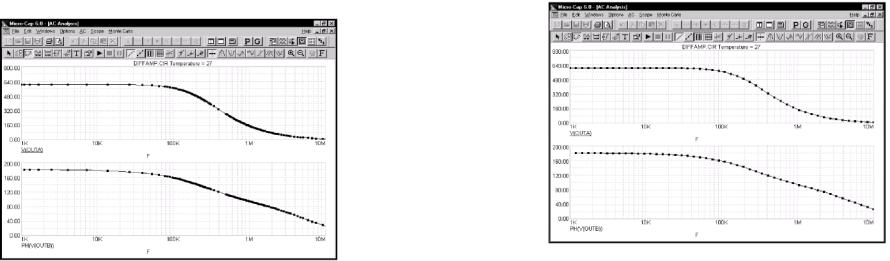
Figure 5-4 The plot with Maximum change % set to 1%

The lower value of 1% produces a smoother plot by calculating more data points. The current Frequency Step method is Auto. In this mode, the frequency step is automatically adjusted to restrain the point-to-point change of both the vertical value and the angle of the plot itself to less than the specified maximum change. The Auto method produces the smoothest plot at the lowest computation price for most curves.

This analysis uses 1% and generates about three times the number of data points as the 5% analysis. Since the analysis time increases in direct proportion to the number of data points, it is wise to keep the Maximum change % as large as possible. A value of 1 to 5 is usually suitable. If the first waveform is very flat, you may want to try a fixed frequency step method.

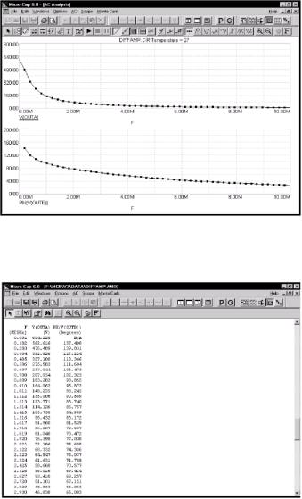
Let's try one of these methods. Press F9 to display the Analysis Limits dialog box. Click in the Frequency Step list box. When the list drops down, click on the Log option. Press F2 to start the run. The result looks like Figure 5-5.

143

Figure 5-5 The plot using the log option

The constant horizontal distance between data points is achieved by making each new frequency a product of the prior frequency and a fixed multiplier. Since the lowest frequency forms the base that is multiplied, it must not be zero.

The Linear option is only used when the X axis is linear. To illustrate, press F9 and edit the Frequency Range field to 1E7,0. Change the Frequency Step method to Linear and change the X Log/Linear button states of the first two waveforms to linear. Press F2 to run. The result looks like Figure 5-6.

Numeric output

To obtain a tabulation of the numerical values simply click the Numer-

ic Output button for each waveform for which numeric output is desired. Do that now for the first two waveforms. Press F9, then click the buttons. Press F2 to run the analysis. All text or numeric output is directed to the Numeric Output window and to a disk file with the name DIFFAMP.ANO. Press F5 to see the window. The first part

144

shows the results of the DC operating point. Scroll down to see the numeric values for the waveforms.

Figure 5-6 The plot using the linear option

The display should look like this:

Figure 5-7 Numeric output

145

A printout of the data in the Numeric Output window may be obtained from the Print option of the File menu.

To display the Analysis Plot window, press F4, or click on the Analysis

Plot button .

To display the Output window, press F5, or click on the Numeric Output button .

Noise plots

MC6 models three types of noise; thermal, shot, and flicker noise. Thermal noise is produced by the random thermal motion of electrons and is always associated with resistance. Discrete resistors and the parasitic resistance of active devices contribute thermal noise.

Shot noise is caused by a random variation in the production of current from a variety of sources including recombination and injection. It is usually associated with dependent current sources. All semiconductor devices generate shot noise.

Flicker noise comes from a variety of sources. In BJTs, the source is contamination traps and other crystal defects that randomly release their captured carriers.

Noise analysis computes the contribution from all these sources as seen at the input and output. Output noise is calculated at the output node specified in the Noise Output field. To plot it, specify ONOISE as the Y expression. Input noise is calculated at the same output node(s) specified in the Noise Output field, but is divided by the gain from the node(s) specified in the Noise Input field to the output node. To plot or print input noise, specify INOISE as the Y expression.

Press F9 and edit the analysis limits to match Figure 5-8. Be sure to disable numeric output for the first two waveforms and to select the Log option.

146

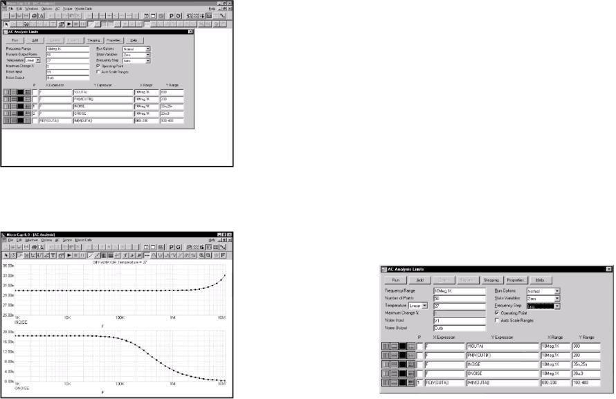
Figure 5-8 The Analysis Limits for Noise plots

Press F2 to run the analysis. The results look like this

Figure 5-9 Plots of input and output noise

In this circuit, thermal noise is generated by the resistors. Shot and flicker noise is generated by the transistors.

Because the equations are structured differently for noise, it is not possible to simultaneously plot noise variables and other types of variables such as voltage and current. That is why we disabled the other waveforms by placing a blank in their P fields. If you attempt to plot both noise and other variables, the program will issue an error message.

Noise is an essentially random process and as a result carries no phase information. For this reason, noise is defined as an RMS quantity. Thus the phase (PH) and group delay (GD) operators will not produce meaningful results when plotting noise. With noise, only magnitudes are meaningful.

The units of noise are V / sqrt(Hz).

Nyquist plots

A Nyquist plot is easy to generate. Edit the analysis limits to look like these. Here we have enabled the last curve and disabled the other curves and selected log stepping.

Figure 5-10 Analysis limits for the Nyquist plot

Press F2 to run the analysis. The result looks like this:

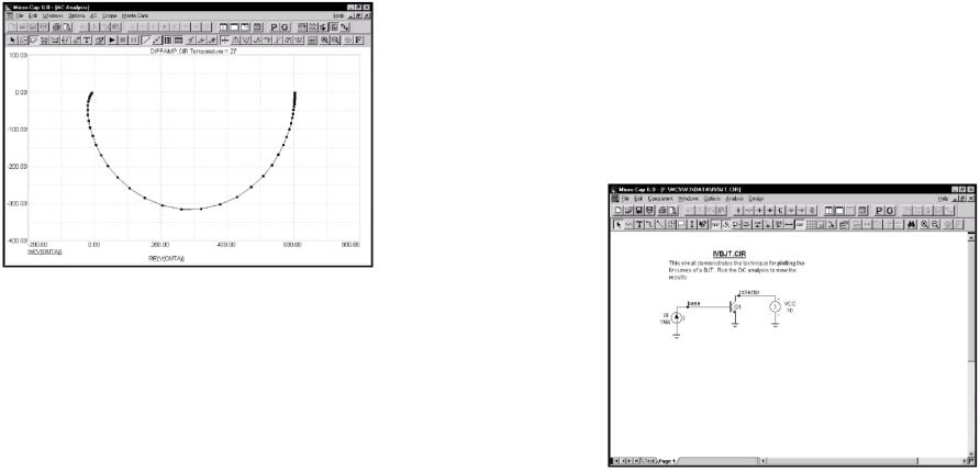
148

Figure 5-11 The Nyquist plot

Note that the X expression in this case was RE(V(OUTA)), not F as it usually is. In general, it can be any expression involving any AC variable

Chapter 6 DC analysis

What's in this chapter

DC analysis is the topic for this chapter. It is a short tutorial covering these subjects:

•What DC analysis does

•What the DC analysis limits do

•A simple circuit for generating IV-curves

DC analysis

In DC analysis, the program treats capacitors as open circuits and inductors as short circuits. It sweeps the specified Variable 1 and solves for the steady-state DC node voltages and branch currents. Two stepping loops are provided for easy creation of parametric

149

plots such as device IV curves. The variable for either loop can be a voltage or current source value, temperature, a model parameter, or a symbolic variable. As in the other analysis routines, the complete set of variables are available for printing and plotting, with the obvious exceptions of charge, flux, capacitance, inductance, В field, and H field. These variables are not provided since flux and charge are ignored in DC analysis. To explore DC analysis, load the file IVBJT. It looks like this:

Figure 6-1 The IVBJT circuit

This circuit is used to plot the I-V characteristics of a bipolar transistor. It can be easily adapted to other device types, such as GaAsFets, MOSFETs, and JFETs. There is a voltage source for the collector voltage sweep and a current source for the base current sweep.

After loading the circuit, select DC Analysis from the Analysis menu. When the DC Analysis Limits dialog box comes up, it looks like Figure 6-2.

150

Figure 6-2 The DC Analysis Limits dialog box

The dialog box instructs MC6 to step the value of the current source IB from 0 to 5 ma, using a maximum step size of 0.5 ma. For each value of the current source, IB, the voltage source, VCC, is to be swept from 0 to 5 volts, using a maximum step size of 1 volt. The step size may be varied during the run to optimize convergence and to conform to the <Maximum change %> constraint, but it is never to be larger than 1 volt. Click on the Run command button and the results look like this:

Figure 6-3 DC analysis plot of I-V characteristics

151

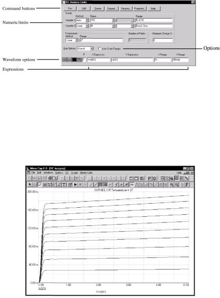
The DC Analysis Limits dialog box

The Analysis Limits dialog box is divided into five major areas: the Command buttons, Sweep group, Waveform options, Expression fields, and Options.

Command buttons. Command buttons provide these commands. Run: This command starts the analysis run. Clicking the Tool bar

Run button or pressing F2 will also start the run.

Add: This command adds another Waveform options field and Expressions field line after the line containing the cursor. The scroll bar to the right of the Expressions field scrolls through the waveforms when needed.

Delete: This command deletes the Waveform option field and Expressions field line where the text cursor is.

Expand: This command expands the working area for the text field where the text cursor currently is. A dialog box is provided for editing or viewing. To use the feature, click in an expression field, then click the Expand button.

Stepping: This command calls up the Stepping dialog box. Stepping is reviewed in a separate chapter.

Properties: This command invokes the Properties dialog box which lets you control the analysis plot window and the way waveforms are displayed. See the Plot Properties dialog box article in Chapter 4, "Transient Analysis".

Help: This command calls up Help information for DC analysis.

Sweep group. The definition of each field in this group is as follows:

• Variable 1: This row specifies the Method, Name, and Range fields for Variable 1. Its value is usually plotted along the X axis. The column fields for this variable are:

• Method: This field specifies one of four methods for sweeping or stepping the variable: Auto, Linear, Log, or List.

152

•Auto: In this mode the rate of step size is adjusted to keep the point-to-point change less than Maximum Change % value.

•Linear: This mode uses the following syntax from the Range column for this row:

<start> [,<end> [,<step>] ]

Start defaults to 0.0. Step defaults to (start - end)/5Q. Variable 1 starts at start. Subsequent values are computed by adding step until end is reached.

• Log: This mode uses the following syntax from the Range column for this row:

<start> [,<end> [,<step>] ]

Start defaults to end/10. Step defaults to exp(ln(end/start*)/Щ.

Variable 1 starts at start. Subsequent values are computed by multiplying by step until end is reached.

• List: This mode uses the following syntax from the Range column for this row:

<vl> [,<v2> [,<v3>] ...[,<vn>] ]

The variable is simply set to each of the values vl, v2, .. vn.

•Name: This field specifies the name of Variable 1. The variable itself may be a source voltage, temperature, a model parameter, or a symbolic parameter (one created with a .DEFINE statement). Model parameter stepping requires both a model name and model parameter name.

•Range: This field specifies the numeric range for the variable. The range syntax depends upon the Method field described above.

•Variable 2: This row specifies the Method, Name, and Range fields for Variable 2. The syntax is the same as for Variable 1, except that the stepping method options include None and exclude Auto. Each

153

discrete value of Variable 2 from the range field produces one complete branch.

• Temperature: This controls the temperature of the run. The fields are:

• Method: This field specifies one of two methods for stepping the temperature: Linear or List.

• Linear: This mode uses the following syntax from the Range column for this row:

<start> [,<end> [,<step>] ]

Start defaults to 0.0. Step defaults to (start - end)/5Q. Variable 1 starts at start. Subsequent values are computed by adding step until end is reached.

• List: This mode uses the following syntax from the Range column for this row:

<vl> [,<v2> [,<v3>] ...[,<vn>] ]

Temperature is simply set to each of the values vl, v2, .. vn. One run is produced for each temperature. Note that when temperature is selected as one of the stepped variables (Variablel or Variable 2) this field is not available.

•Range: This field specifies the range for the temperature variable. The range syntax depends upon the Method field described above.

•Number of Points: This is the number of data points to be interpolated and printed if numeric output is requested. This number defaults to 51 and is usually set to an odd value to produce an even print interval. Its value is:

(<finall> - <initiall> ) l(<Number of points> - 1)

<Number ofpoints> values are printed for each value of the Input 2 source.

154

• Maximum Change %: This value is only used if Auto is selected as the step method for Variable 1.

The Waveform options are located below the Numeric limits and to the left of the Expressions. Waveform options affect the waveform in the same row. The definition of each option is as follows:

The first option toggles the X-axis between a linear and a log plot. Log plots require positive scale ranges.

Waveform options

The second option toggles the Y-axis between a linear and a log

plot. Log plots require positive scale ranges.

The option activates the color menu. There are 64 color choices for an individual curve. The button color is the curve color.

The option prints a table showing the numeric value of the curve. The number of values printed is controlled by the Number of Points value. The table is printed to the Numeric Output window and saved in the file CIRCUITNAME.DNO.

A number from 1 to 9 is used in the Plot (P) column to group the curves into different plots. All waveforms with like numbers are placed in the same plot. If the P column is blank, the waveform is not plotted.

Expressions

The Expressions field is used to specify the horizontal (X) and vertical

(Y) scale ranges and expressions. Some common expressions used are VCE(Ql) (collector to emitter voltage of transistor Ql) or IB(Q1) (base current of transistor Ql). The scale ranges specify the scales to be used when plotting the X and Y expressions. The range format is:

<high> [, <low>]

155

<low> defaults to zero. You may also enter "AUTO" and the program determines the scale range automatically.

Clicking the right mouse button in the Y expression field invokes the Variables list which lets you select variables, constants, functions, and operators, or expand the field to allow editing long expressions. Clicking the right mouse button in the other fields invokes a simpler menu showing suitable choices.

Options

The Options are to the right of the Numeric limits. The Auto Scale Ranges option has a check box. Clicking the mouse in the box will toggle the options on or off with an X in the box showing that the option is enabled. The options available from here are:

•Run ptions

•Normal: This runs the simulation without saving it to disk.

•Save: This runs the simulation and saves it to disk.

•Retrieve: This loads a previously saved simulation and plots and prints it as if it were a new run.

•Auto Scale Ranges: This sets the X and Y range to auto every time a simulation is run. If it is disabled, the values from the range fields will be used.

Press F3 and unload the IVBJT circuit without saving it.

156

Учебное издание

Каширский Сергей Николаевич Литвиненко Владимир Петрович Токарев Антон Борисович

Система схемотехнического моделирования

Micro-Cap 6.0

Пособие для обучения переводу и чтению на английском языке

для радиоэлектронных специальностей

Часть 1

Компьютерный набор В.П. Литвиненко

ЛР № 066815 от 25.08.99. Подписано к изданию 28.10.03. Уч.-изд. л. 5,3

394026 Воронеж, Московский просп., 14

НОУ ШКОЛА «ДРИМ-DREAM»

для ВСЕХ!!!

Лицензия г653288 ГУО-168АВО

Админ. Вор. обл. от 16 апреля 2002г.

- Бизнесменам – Выезжающим за рубеж - Аспирантам – Школьникам – Малышам –

Вузовские педагоги

Лондонские, Оксфордские, Кембриджские аудиокурсы

Приемлемые цены

Быстро и качественно

Занятия проводятся в филиалах города.