2891

This moves the insertion point. Press CTRL + V to paste the contents of the clipboard to the insertion point. Your circuit should now look like this:

Figure 3-18 After pasting the clipboard contents

The saved region has been copied, or pasted, from the clipboard to the schematic.

Selection

Single objects or entire regions may be selected for editing, deleting, moving, rotating, mirroring, stepping, or copying. They may be selected or deselected individually or as a group. Clicking on an object or region while the SHIFT key is down toggles the selection state. If the object or region was formerly selected, it becomes deselected. If it was formerly deselected, it becomes selected.

To illustrate, press the SHIFT key and hold it down. Click on the Q7 transistor in the selected group. Be careful not to click on the name Q7 as that will select the PART attribute rather than the part itself. Release the SHIFT key and the circuit looks like this:

99

Figure 3-19 Partial selection using SHIFT + mouse click

The left transistor is now deselected. If you press the Del key, the transistor will remain but the rest of the selected region will be deleted. Press the SHIFT key and click the same transistor and it is again selected. If you now press the Del key, the entire selected region will be deleted.

By using partial selection, virtually any subset of a schematic can be selected for editing, copying, deleting, or moving.

To complete this part of the tutorial, click on the Revert button to restore the DIFFAMP circuit.

Drag copying

Ordinarily, when you drag a selected object or group of objects, the entire group moves with the mouse. However, if you hold down the CTRL key while you drag, MC6 leaves the original selected objects in place, makes a copy, and drags the copy along with the mouse. It's like tearing off a sheet from a pad of printed copies. As with stepping and clipboard pasting, the part names are incremented. Grid text is incremented only if the Options / Preferences / Common Options / Text Increment option is enabled.

100

To illustrate with the DIFFAMP circuit, click on the Select button, and drag a region box around the V2 battery at the upper right. Release the button. Press CTRL. Click within the selected region and drag it to the right. Notice that a copy of the selected region is created as shown below.

Figure 3-20 Drag copying

Drag copying is usually more convenient than clipboard cut and paste when you need to make only one copy. Its one step operation is easier and simpler to use than copying and pasting from the clipboard.

If you plan to paste more than one copy, then copying and pasting from the clipboard is usually faster.

Pan means to move the window view.

Navigating large schematics

How do you navigate a large a schematic?

1.Use the schematic scroll bars. This is slow but sure.

2.Use the Zoom-Out or Zoom-In buttons in the Tool

bar.

101

3.Use the keyboard or the right mouse button to pan. Keyboard panning usesCTRL + <any cursor key> to move the view in the direction of the arrow. Mouse panning involves clicking and holding down the right mouse button, while dragging the mouse. It's like sliding a piece of paper across a desktop.

3.Use the SHIFT + click method to relocate and change views. While holding down the SHIFT button, click the right mouse button at the point youwant centered in the window. Clicking toggles the scale between 1:1 and .5:1 and centers the schematic at the mouse position.

4.Place flags at locations you expect to revisit. Then select a flag from the list by clicking on the flag icon in the lower right corner of the window.

5.Use the Page scroll bar if the desired area is on another page. You can also use CTRL + PAGE UP and CTRL + PAGE DOWN to navigate the pages.

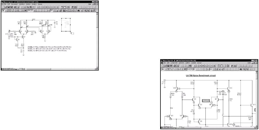
Figure 3-21 The UA709 circuit

To illustrate these methods, load the circuit UA709. It looks like Figure 3-21. At a resolution of 600 X 800, it's too large to see at the default scale, so shrink its scale by clicking twice on the Zoom-Out button. At 102

this scale the circuit looks like this:

Figure 3-22 After clicking the Zoom-Out button

The Zoom-In button increases the image size

The Zoom-Out button decreases the image size

Simultaneously press the SHIFT key and click the right mouse button in the lower right, near the two transistors. This centers the schematic at the mouse position and redraws it at normal scale.

Figure 3-23 The UA709 after repositioning

103

Another SHIFT + click redraws the circuit at .5:1 scale. A final SHIFT + click near the upper left corner returns the schematic to 1:1 scale.

Panning uses the keyboard cursor keys or a right button mouse drag to move the schematic.

Panning is probably the easiest and most powerful method of moving around most schematics. To pan, drag anywhere on the schematic using the right mouse button. While holding the button down, drag the mouse and move the schematic. When the mouse is at or near a window edge, release the mouse button. Repeat the procedure until the schematic is in the desired position. Pan the UA709 circuit by clicking near the center and dragging left. This moves the schematic to the left, exposing more of the right-hand portion.

Finally, you can use flags to navigate the schematic. This method is most useful for very large schematics where panning might take many attempts to span the entire schematic. In this method you place flags in the schematic where you expect to want to visit in the future. Then simply picking the flag from the list centers the schematic view around the selected flag. To illustrate, click on the Flag icon, and from the list that pops up, select the 'DIFFPAIR' flag. This redraws the schematic, centered on the flag, as shown below.

Figure 3-24 Navigating with flags

104

Note that there is a Flag button in the Tool bar and a Flag icon in the

lower right corner of the window. The Flag button activates the Flag mode which lets mouse clicks place flags in the schematic. The Flag icon displays a list from which a flag is selected for viewing.

Close the UA709 file without saving it.

Creating and editing SPICE text files

MC6 can create and analyze SPICE text file circuit descriptions as well as schematics. SPICE text files may be created externally with a word processor or text editor, or internally using the MC6 text editor. To illustrate the procedure for creating a text file, select the New option from the File menu. This presents a dialog box where you specify the type of file to create. Click on the SPICE/Text option, then on the OK button. This opens a new text window and positions the text cursor at the upper left.

Type in the following:

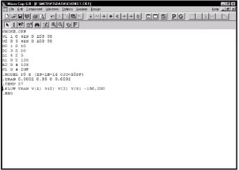
CHOKE.CKT

VI 1 0 SIN (0 100 50)

V2 0 3 SIN (0 100 50) DO 1 2 DO

D132DO LI 4 25 Rl 0 210K

R2 0 4 10K

C2 0 4 2UF

.MODEL DO D (IS=1E-14 CJO=10PF)

.TRAN 0.0002 0.05 0 .0002

.TEMP 27

.PLOT TRAN V(l) V(2) V(3) V(4) -150, 200

.END

105

Save the circuit under the name CHOKEl.CKT using the Save As option from the File menu. Note that SPICE circuit file names do not require or assume an extension. There is no default extension. Any extension except "CIR" can be used. The "CIR" extension is reserved for schematic files. By convention, MC6 uses "CKT" for SPICE files, but any extension, except "CIR", will do.

New SPICE/Text files are created in the same way as schematics, by using the New command from the File menu.

Figure 3-25 The sample SPICE circuit

Your circuit should look like Figure 3-25. Press ALT + 1 to run a transient analysis. When the Analysis Limits dialog box is displayed, press F2 to run the analysis. The results should look like Figure 3-26.

After the analysis the program automatically determines suitable scales if needed and plots the requested waveforms as specified in the

.PLOT statement.

Exit the analysis by pressing F3, then close the file with CTRL + F4

106

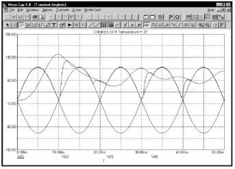
Figure 3-26 Transient analysis of the SPICE circuit

.

Summary

The most important ideas and methods covered in this chapter are:

•To open a new schematic use the New item on the File menu, or use the one automatically opened when the program first starts.

•Change the default component if it is different from the one you want to\ add. Default components are selected from the Component menu, a Component palette, or one of the part buttons in the Tool menu.

•To add a component, press CTRL + D or click the Component mode button. Select the component you want from the Component menu, User palette, or Tool bar button. Click the mouse on the schematic and drag it into place. If necessary, change its orientation with the right mouse button.

•Press CTRL + W or click the Wire item in the Tool bar to add wires.

107

•Components are connected with wires. To add a wire, click at one endpoint, drag the mouse to the other endpoint, then release it. Crossing wires do not connect.

•Press CTRL + Т or click the Text button in the Tool bar to add text.

•Add text to nodes to name them for easy reference or use the node numbers. Nodes with the same name are connected.

•To edit, move, copy to the clipboard, or delete an object, it must first be selected. To select an object, press CTRL + E to enter the Select mode, then click the object. To select a region, drag the mouse over the region. Use SHIFT + click to deselect an object in a selected group.

•Selected objects are copied to the clipboard with CTRL + С and pasted to the cursor location with CTRL + V.

•CTRL + drag copies and renames selected objects.

Navigating a schematic is done by scrolling, panning, changing the scale, positioning with SHIFT + click, using flags, and page scrolling.

108

Chapter 4 Transient Analysis

Ответьте на вопросы:

1.Что необходимо сделать для составления графика различных форм волн?

2.Скажите в каком абзаце текста говорится о:

а) рабочей точке б) операции Zero

в) автодиапазонах шкалы

3.Скажите, что говорится в тексте о: а) числовых пределах б) списке переменных

в) диалоговом окне Plot Properties

4.Найдите примеры, которые доказывают следующие утверждения:

а) чтобы вызвать диалоговое окно для графика нажмите

F10

б) кнопка “продвижения” вызывает диалоговое окно

Stepping

в) команда “сохранение” выполняет моделирование и сохраняет данные на диске (файл с именем

CIRCUITNAME.TSA)

What's in this chapter

Transient analysis is the topic of this chapter. Using the MIXED4 circuit, the capabilities of the time domain simulator are explored. The goal is to introduce and build a sound understanding of these basic subjects:

•Controlling the analysis through the Analysis Limits dialog box

•Selecting waveforms to plot or print

•State variables and initialization

•State Variables editor

109

The Transient Analysis Limits dialog box

Load the MIXED4 circuit file and select Transient from the Analysis menu. MC6 extracts the necessary circuit information directly from the schematic. More information is needed before the analysis can begin, and that information is supplied by the Analysis Limits dialog box.

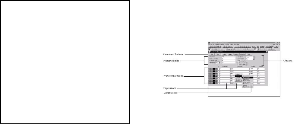
The Analysis Limits dialog box is divided into five areas: the Command buttons, Numeric limits, Waveform options, Expression fields, and Options.

Figure 4-1 The Analysis Limits dialog box

Command buttons

The Command buttons, located just above the Numeric limits field, contain seven commands.

Run: This command starts the analysis run. Clicking the Tool bar Run

button or pressing F2 will also start the run.

Add: This command adds another Waveform options field and Expression field line after the line containing the cursor. The scroll bar to the right of the Expression field scrolls through the waveforms when there are more than can be displayed.

Delete: This command deletes the Waveform option field and Expression field line where the text cursor is.

110

Expand: This command expands the text field where the text cursor is into a large dialog box for editing or viewing. To use the feature, click the mouse in the desired text field, and then click the Expand button.

Stepping: This command invokes the Stepping dialog box. Stepping is reviewed in a separate chapter.

Properties: This command invokes the Properties dialog box which lets you control the analysis plot window and the way waveforms are displayed.

Help: This command invokes the Help Screen. The Help system provides information by index and topic.

Numeric limits

The Numeric limits field provides control over the analysis time range, time step, number of printed points, and the temperature(s) to be used.

•Time Range: This field determines the start and stop time for the analysis.

The format of the field is:

<tmax> [,<tmin>]

The run starts with time set equal to <tmin>, which defaults to zero, and ends when time equals <tmax>.

•Maximum Time Step: This field defines the maximum time step that the program is allowed to use. The default value, (<tmax>- <tmin>)/50, is used when the entry is blank or 0.

•Number of Points: The contents of this field determine the number of printed values in the numeric output. The default value is 51. Note that this number is usually set to an odd value to produce an even print interval. The print interval is the time separation between successive printouts. The print interval used is:

print interval = (<tmax> - <tmin>)/([number of points] - 1)

•Temperature: This field specifies the global temperature of the run. This temperature is used for each device unless individual device temperatures are specified. If the Temperature list box shows Linear the format is:

111

<high> [, <low> [, <step> ] ]

The values are in degrees Celsius. The default value of <low> is

<high>, and the default value of <step> is <high> - <low>.

If the Temperature list box shows List the format is:

<tl> [, <t2> [, <tf> ] [,...]] where tl, t2,.. are individual values of temperature.

One run is produced for each requested temperature, producing multiple branches of each waveform.

Waveform options

The Waveform options field is located below the Numeric limits field and to the left of the Expressions field. Each waveform option affects only the waveform in its row. The options function as follows:

The first option toggles the X-axis between a linear and a log plot. Log plots require positive scale ranges.

The second option toggles the Y-axis between a linear and a log plot. Log plots require positive scale ranges.

The option activates the color menu. There are 64 color choices for an individual waveform. The button color is the waveform color.

The option prints a table of the waveform's numeric values. The number of values printed is set by the Number of Points value. The table is printed to the Numeric Output window and saved in the file CIRCUITNAME.TNO.

A number from 1 to 9 in the Plot (P) column is used to group the waveforms into different plots. All waveforms with like numbers are placed in the same plot. If the P column is blank, the waveform is not plotted.

112

Expressions

The X Expression and Y Expression fields specify the horizontal (X) and vertical (Y) expressions. MC6 can evaluate and plot a wide variety of expressions for either scale. Usually these are single variables like Т (time), V(10) (voltage at node 10), or D(OUT) (digital state of node OUT), but the expressions can be more elaborate like V(2,3)*I(Vl)*sin(2*PI*lE6*T).

Variables list

Clicking the right mouse button in the Y expression field invokes the Variables list which lets you select variables, constants, functions, and operators, or expand the field to allow editing long expressions. Clicking the right mouse button in the other fields invokes a simpler menu showing suitable choices.

The X Range and Y Range fields specify the numeric scales to be used when plotting the X and Y expressions.

The format is:

<high> [,<low>]

<low> defaults to zero. Use the word "AUTO" in the scale range to have MC6 determine an individual range automatically, or you can select the Auto Scale Ranges option to scale all ranges after the run and copy the values to the X Range and Y Range fields. The Auto Scale (F6) command can be used to scale all waveforms after the run, but it doesn't overwrite the Analysis Limits range values, letting you restore them with CTRL+HOME if needed.

These options include the following:

•Run Options

•Normal: This runs the simulation without saving it.

•Save: This runs the simulation and saves it to disk, using the same format as in Probe. The file name is CIRCUITNAME.TSA.

113

•Retrieve: This loads a previously saved simulation and plots and prints it as if it were a new run. The file name is CIRCUITNAME.TSA.

•State Variables

These options determine the state variables at the start of the next run.

•Zero: This sets the state variable initial values (node voltages, inductor currents, digital states) to zero or X.

•Read: This reads a previously saved set of state variables and uses them as the initial values for the run.

•Leave: This leaves the current values of state variables alone. They retain their last values. If this is the first run, they are zero. If you have just run an analysis without returning to the Schematic editor, they are the values at the end of the run. If the run was an operating point only run, the values are the DC operating point.

•Operating Point: This calculates a DC operating point. It uses the initial state variables as a starting point and calculates a new set that represents the DC steady state response of the circuit to the T=0 values of all sources.

•Operating Point Only: This calculates a DC operating point only. No transient run is made. The state variables are left with their final operating point values.

•Auto Scale Ranges: This sets the X and Y range to AUTO for each new analysis run. If it is not enabled, the existing scale values from the X and Y Range fields are used.

The Run, State Variables, and Analysis options affect the simulation results. To see the effect of changes of these options you must do a run by clicking on the Run command button or pressing F2.

Selecting waveforms to plot or print

Note: MC6 initially selects the voltage waveforms of the first two named nodes for plotting.

114

MC6 automatically creates a set of analysis limits for newly created circuits. It tries to guess what waveforms you may want to look at and what plot and analysis options you may want. Usually, it is necessary to change these initial guesses. Changes you make to any entry in the Analysis Limits dialog box are saved with the circuit file, so you don't need to enter these each time you run.

Click on the Run button to do the transient analysis of the MIXED4 circuit.

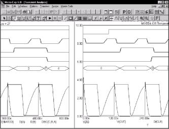
The first five waveforms are digital and show the CLR input, clock input, the state outputs of the first two flip-flops, and the decimal value of the three flip-flop outputs. The next two waveforms are plots of the voltage at the input pulse source and the output of the analog section. In general, V(A) plots the voltage on an analog node A. D(B) plots the state of a digital node B.

Figure 4-2 Transient analysis of MIXED4

Plotting other waveforms

You can plot expressions using a variety of variables such as node voltage or device terminal voltage or current. To plot different 115

waveforms, you can add new waveform fields or you can change existing waveform fields. To illustrate, press F9 to display the Analysis Limits dialog box. Click in any column of the last waveform row. Click the Add button in the upper part of the dialog box. This adds a new waveform row and moves the text cursor to the P column of the new row. It also duplicates the contents of all fields of the row above. Click the Delete button. This deletes the waveform just added. Click the Add button to add the waveform row back. Since we want the new waveforms to be placed on a separate plot, change the Т in the P column to '2'. Press the Tab key twice or click the mouse in the Y Expression field. Type in the following:

"IC(Q4)*VCE(Q4)"

Press the Tab key twice to move the cursor to the Y Range field and type "Auto". This tells the program to determine the Y scale range automatically, after the run. During the run, MC6 uses a default scale to plot the waveform. This sometimes means that the waveform can't be seen during the run. When the run is complete, MC6 determines the scale necessary to show the complete waveform, plots it, and enters the new scales into the X and Y range fields.

What if you can't remember the variable or function name you want? Use the Variables list. To illustrate, click the Add button again. Click in the new Y Expression field with the left mouse button and drag select the entire Y expression. Click on the selected Y expression with the right mouse button. This invokes the Variables list, a small pop-up menu that lets you select variables, functions, and operators. It also lets you expand the limited text editing area to a full size text edit dialog box. This is handy for complex expressions with many parentheses. Click on Variables and then on Device Currents. This displays a dialog box with a list of the available device currents in the circuit. Click on I(VCC). Click the OK button. The text "I(VCC)" is entered in the Y Expression field and the cursor is placed to the right of the text. The Y expression will now look like this:

116

I(VCC)

Type "*". Click the right mouse button and select Variables / Device Voltages / V(VCC). Click OK. The Y expression should now look like this:

I(VCC)*V(VCC)

Press the Home key to move the cursor to the start of the field. Click the right mouse button and click Functions / Calculus / SUM. SUM is the integration operator. It integrates the expression to the right of the text cursor, with respect to the X expression variable, T. Press the End key to put the cursor at the end of the field and type "/T". This produces an expression for the average power supplied by the VCC battery. The Y expression should now look like this:

SUM(I(VCC) * V(VCC),T)/T

Since the new waveform was created with AUTO in the Y Range field we do not need to edit that field. After the run, MC6 will determine the actual waveform range and calculate a suitable Y scale. Because there are two waveforms sharing the same plot group, it can do this two ways; 1) by finding a common scale large enough to show all of both graphs, or 2) by finding an individual scale for each waveform and printing two Y scales. The choice is determined by the Same Y Scales option on the Scope menu. If this option is checked, then all waveforms in each plot group will share a common scale large enough to plot all parts of each waveform. This is true regardless of whether auto or user-specified scales are used. If you select this option, MC6 draws a single scale using the largest of the specified or calculated scales. Click the Run button. Here is how the new run looks when the option is disabled.

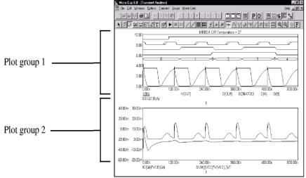
Figure 4-3 Transient analysis with two plot groups

Group 1 contains the original waveforms. Group 2 contains the new waveforms: the instantaneous collector power of the output transistor Q4, and the average power supplied by the VCC battery. Plot grouping is specified by the P column number. All waveforms with the same number are plotted in the same group.

Analog and digital waveforms may be grouped together or separately. When grouped together, digital waveforms are plotted in the same order they occur in the dialog box, starting at the top of the graph. Analog waveforms are plotted using the range scales, which only apply to analog waveforms. This can cause the waveforms to overlap. Overlap can be minimized by compressing the analog waveforms with a large Y Range value. Separating analog and digital into groups avoids overlap but is less convenient when comparing the two sets of waveforms at the same time value