

2891
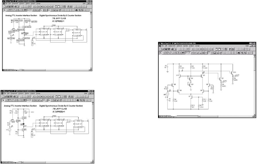
.pdfFigure 2-1 The MIXED4 sample circuit
The circuit employs an analog TTL inverter to drive a digital three-stage synchronous divide-by-five counter. The digital clock input to the first JK flip-flop is driven by the analog TTL output, while the CLRB initializing pulse for the flip-flops is provided by a digital source, U2. The CLKB inputs are tied together with a .TIE command. The flip-flop preset nodes are connected together by a wire and the node is labeled PREB with grid text. This node is initialized to a T state with an .1C command. The digital source states are specified in a .DEFINE command statement located in the schematic text area. The text area is a private cache in each schematic for storing text. You can toggle the display between the drawing and text areas by pressing CTRL + G or by clicking on the Text tab in the lower page scroll bar. This combination of analog and digital circuitry is easily handled by the program, since it contains a native, event-driven digital simulation engine, internally synchronized with its SPICE-based analog simulation engine. Mi- cro-Cap 6 is a true mixed-signal simulator.
19
Transient analysis display
Select Transient from the Analysis menu. MC6 presents the Analysis Limits dialog box. Here you specify the simulation time range, choose plot and simulation options, and select waveforms to be plotted during the run.
Figure 2-2 The Analysis Limits dialog box
Here we have chosen to plot the analog voltage waveforms at the input pulse source, the output of the analog section, and several of the digital waveforms. In general, MC6 can plot any expression using as variables any node voltage or state or any device terminal voltage or current. Here are a few examples of expressions that could be plotted.
There are a great many other variables available for plotting. Click the right mouse button in the Y Expression field to see a list of variables available for plotting or printing. Click outside of the menu to remove it.
20
Now let's run the actual simulation. Click on the Run button  or press F2 to start the simulation. MC6 plots the results during the run.
The run can be stopped at any time by clicking the Stop button  or by pressing ESC.
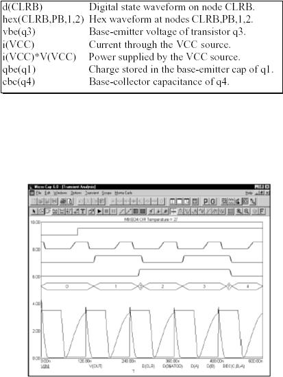
Figure 2-3 Transient analysis of the circuit
The final waveforms look like Figure 2-3. Each waveform can have its own token, width, pattern, and color. These options are set from Options / Default Properties for New Circuits for new circuits and 21
can be changed for the current circuit from the Properties (F10) dialog box. Waveforms can be grouped into one or more plots. Grouping is controlled by the plot number assigned to each waveform. The plot number is the number in the P column of the Analysis Limits dialog box. You can assign all the waveforms to a single plot, or group them into as many plots as will fit on the screen. To assign several waveforms to the same plot, give them all the same plot number. To create several plots, use different plot numbers. To disable plotting a waveform, enter a blank for the plot number.
In this example, all waveforms in the plot group share a common vertical scale. You can use different scales by 1) disabling the Scope / Same Y Scales option and 2) specifying the scales you want in the Y Range field. All waveforms in a plot group always share the same horizontal or X scale.
Digital and analog waveforms may be mixed or separated. Separated digital waveforms show the expression on the left, adjacent to the plot. Mixed digital waveforms display the expression at the bottom of the plot along with the analog expressions in the order of their occurrence in the Analysis Limits dialog box.
Zooming in on a waveform
Place the mouse near the top middle of the waveform plot group. Press the left mouse button and while holding it down, slide the mouse down and to the right to create an outline box as shown in the figure below.
Release the mouse button and MC6 magnifies and redraws the box region.
If you make a mistake, press CTRL + HOME and try again.
Press F3 to quit the analysis. Select Dynamic DC from the Analysis
menu. This runs a DC operating point. Click on the  button to display the node voltages and digital states like this:
22
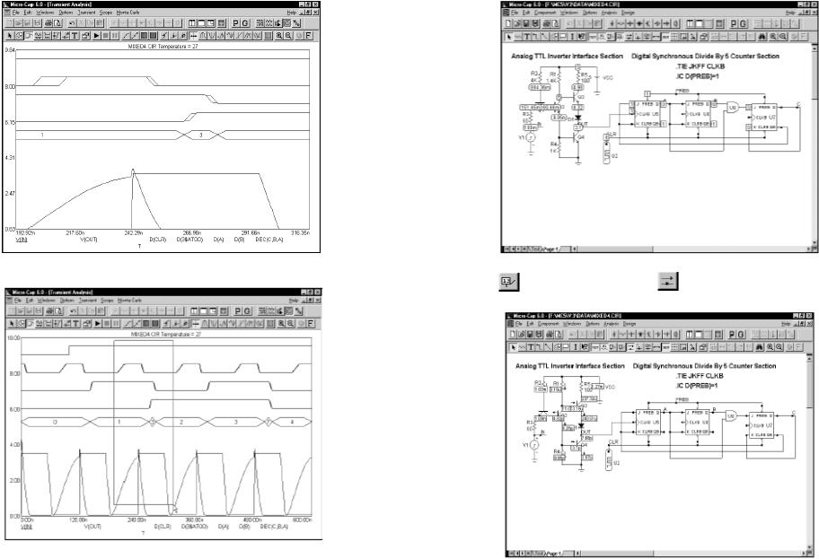
Figure 2-4 Using the mouse to magnify a waveform |
Figure 2-6 Operating point node voltages and states |
|
Click |
to turn off voltages and |
to display currents like this: |
Figure 2-5 The magnified region
Figure 2-7 Operating point DC currents
23 |
24 |
Click  to turn off currents and
  to display power terms like this:
Figure 2-8 Operating point DC power terms
Click  to turn off power and
  to display conditions like this:
Figure 2-9 Operating point DC conditions
25
The voltage, current, power, and condition displays show present time-domain values, which are usually the result of a DC operating point.
AC analysis
Turn off the Dynamic DC analysis mode from the Analysis menu. Remove the MIXED4 circuit by choosing Close from the File menu. Load a new file by choosing Open from the File menu. Type RCA3040 for the name. Click Open.
Figure 2-10 The RCA3040 circuit
Select AC from the Analysis menu. As before, an analysis limits dialog box appears. We have chosen to plot the voltage of the two nodes, Outl and Out2, in dB. Click on the Run button, and the analysis plot looks like this:
26
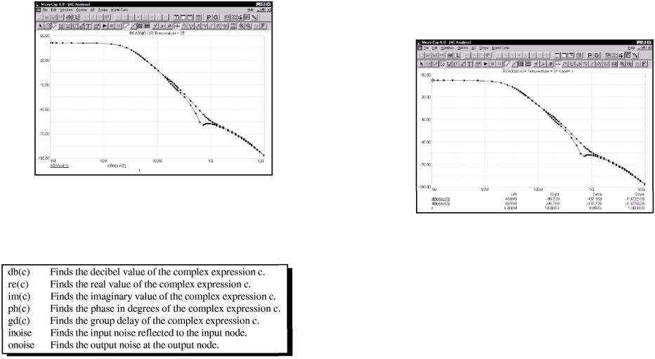
Figure 2-11 AC analysis plot
The same rich set of expressions available in transient analysis is also available in AC analysis. In addition, these operators are very useful:
Scope in Cursor mode
Click on the Cursor mode button  in the Tool bar or press F8. In this mode, two cursors are placed on the graphand may be moved about. The table below the plots show the waveform values at each of the two cursors, the difference between them, and the 27
slope. Click the left and right mouse buttons somewhere near the middle of the graph. The display should look like this:
Figure 2-12 The Cursor mode
The left mouse button controls the left cursor and the right button controls the right cursor. The cursor keys LEFT ARROW and RIGHT ARROW also control the cursors. As the cursors move around, the numeric display continuously updates to show the value of the waveforms, the change in waveforms between the two cursors, and the waveform slope between the two cursors. Press F3 to exit the AC analysis routine. Choose Close from the File menu to unload the circuit.
DC analysis
Choose Open from the File menu to load a new circuit, then type "IVBJT" and click the Open button.
28

Figure 2-13 The IVBJT circuit
This creates a set of bipolar transistor IV curves. Choose DC from the Analysis menu. Click on the Run button. The plots look like this:
Figure 2-14 The IV curves of a bipolar transistor
Press F3 to exit the DC analysis, then unload the circuit with CTRL + F4.
Probe
Probe is the final topic on our quick tour of MC6. Press CTRL + O, then type "MIXED4". Click Open. Choose Probe Transient from the Analysis menu. MC6 runs the analysis, saves it to disk, and presents the Probe display. You scroll the schematic or pan it with a click and drag of the right mouse button and probe any node or component with a click of the left mouse button. Move the mouse to the pulse source and click the left button on the dot near the IN node, and its voltage waveform is fetched from disk and plotted. Click the mouse on the dot near the OUT node, on the dot near the CLKB JK input pin, and on the CLR node. This plots the analog input and output, and the clock and CLR digital waveforms. Analog and digital waveforms are placed in the same plot when the Separate Analog and Digital option on the Probe menu is not checked.
Figure 2-15 The Probe display
29 |
30 |
Probing on a node produces either analog node voltage waveforms or digital node state waveforms. Probing between the leads of an analog device produces pin to pin terminal voltage waveforms such as VBE(Q4). Probing on a digital device produces a list of the pin names. Selecting a pin name from this list plots the digital waveform on that pin. Current waveforms are also available, as are charge, capacitance, inductance, flux, and all the usual variables. In addition, you can enter expressions involving circuit variables.
Press F3 to exit the Probe routines and return to the Schematic editor. Remove the circuit with CTRL + F4. This completes the quick tour. For more extensive tours of MC6, see the Demo options in the Help menu.
Command line format
Command lines and batch files
Although Micro-Cap 6 is designed to run primarily in an interactive mode, it can also be run as a batch process from the Program Manager command line. Either of two formats may be used.
MC6 [F1[.EXT]]...[FN[.EXT]]
MC6 [ [/S I /R] I [[/P] I [/PC I /PA ]]] [@BATCH.BAT]
In the first format, Fl, ...FN are the names of one or more circuit files to be loaded. The program loads the circuit files and awaits further commands.
Batch mode format
In the second format, circuits can be simulated in batch mode by including the circuit name and the analysis type, /T(transient), /A(AC), or /D(DC) on a line in a text file. The syntax of the circuit line inside the batch file is:
CIRCUITNAME [ [/T /A /D] [/S I /R] I [[/P] I [/PC I
31
The definition of each command is as follows:
/T |
Run transient analysis on the circuit. |
/A |
Run AC analysis on the circuit. |
/D |
Run DC analysis on the circuit. |
/S |
Save the analysis run to disk for later recall. |
/R |
Retrieve the analysis run from disk and plot the |
|
waveforms specified in the Analysis Limits dialog box. |
/PC |
Print the circuit diagram. |
/PA |
Print the circuit analysis plot. |
/P |
Print the circuit diagram and analysis plot. |
The /T, /A, and /D commands are for the batch file lines only. The other commands may be applied globally for all circuits in the batch file by placing them on the Program Manager command line, or locally to a particular circuit file by placing them on a circuit line within the batch file.
In the second format, MC6 must be invoked with the name of the batch file preceded by the character '@'. For example, consider a text file called TEST.BAT containing these three lines:
PRLC /A /T SENSOR.CK T /A LOGIC /T
If MC6 is invoked with the command line, MC6 @TEST.BAT, it will:
1.Load the PRLC.CIR circuit and run an AC and transient analysis.
2.Load the SENSOR.CKT circuit and run an AC analysis.
3.Load the LOGIC.CIR circuit and run a transient analysis.
During these analyses, the expressions specified in the circuit file would be plotted during the run and be visible on the screen, but the results would not be saved to disk.
Note that the default circuit file name extension is .CIR. 32

By appending an VS' to the command line, all of the analyses specified in the batch file will be run and the results saved to disk for later recall. By appending an VR' to the command line the analyses are bypassed and the results merely recalled and plotted.
By appending a VP' to the command line, all of the analyses specified in the batch file will be run and the circuit and analysis plot printed.
Terms and concepts
Here are some of the important terms and concepts used in the program.
Attribute. Components use attributes to identify part names, model names, and other defining characteristics. Attributes are created and edited in the Attributes dialog box which is accessed by doubleclicking on the component.
Box. The box is a rectangular region of a circuit or an analysis plot. Created by a drag operation, it defines plot regions to be magnified or circuit regions to be stepped, deleted, rotated, moved, turned into a macro, or copied to the clipboard.
Click the mouse. Most mice have two or more buttons. 'Click the mouse' means to press and release either the left or right button. The middle button is not used.
Clipboard. This is a temporary storage area for whole or partial circuits from a schematic, or text from any text entry field. Items are copied to the clipboard with the Copy command (CTRL + C) and pasted (CTRL + V) from the clipboard into the current schematic or data field with the Paste command. Anything that is cut is also copied to the clipboard. Anything that is cleared or deleted is not copied to the clipboard.
33
Component. A component is any electrical circuit object. This includes connectors, macros, and all electrical devices. This excludes grid text, wires, pictures, and graphical objects.
Copy. This command (CTRL + C) copies text from a text field or circuit objects from a schematic to the clipboard for use with the Paste command (CTRL + V).
Найдите ответы на вопросы:
1.Что означает термин Disabled?
2.Что означает термин Drag?
3.Функция клавиши ESC?
4.Что такое Node?
5.Что происходит при нажатии клавиш CTRL+V?
6.Что представляет собой схематический редактор?
7.Какие функциональные возможности меню Вы знаете?
Cursor. The cursor marks the insertion point. When an object is inserted into a circuit or text inserted into a text entry field, it is placed at the cursor site. The schematic cursor is a mouse arrow or the actual component shape, depending upon a user-selected option. The text cursor is a flashing vertical bar.
Disabled. This means temporarily unavailable. See Enabled.
Drag. A drag operation involves pressing the mouse button, and while holding it down, dragging the mouse to a new location. Dragging with the right button is used for panning shape displays, circuit schematics and analysis plots. Dragging with the left button is used for box region selection, drag copying, moving circuit objects, and magnifying an analysis plot region.
34
Enabled. A check box button feature is enabled by clicking it with the mouse. It shows an X when enabled. A menu item feature is enabled by clicking it to show a check mark. A button feature is enabled by clicking it to depress the button. Button features are disabled by clicking them to release the button. Other features are disabled when they show neither an X nor a check mark.
ESC. The ESC key is used as a single key alternative to closing the Shape editor, Component editor, Stepping, Monte Carlo, and State Variables dialog boxes and to stop a simulation. It is equivalent to Cancel in a dialog box.
Grid. The grid is a rectangular array of equally spaced locations in the circuit that defines all possible locations for the origin of circuit objects. The grid can be seen by clicking on the Grid icon.
Grid text. This refers to any text placed in a schematic. It is called grid text to distinguish it from component attribute text. Grid text may be placed anywhere. Attribute text is always adjacent to and moves with the component. When grid text is placed on a node it gives the node a name which can be used in expressions. Grid text may be moved back and forth between a schematic page and the schematic text area by selecting the text and pressing CTRL + B.
Wire. Wires connect one or more nodes together. Crossing wires do not connect. Wires that terminate on other wires are connected together. A dot signifying a connection is placed where a wire connects to another wire or to a component pin. Two wires placed end- to-end are fused into a single wire.
Macro. A macro is a schematic, created and saved on disk to be used as a component in other schematics. It uses pin names to specify its connections to the calling circuit.
35
Node. A node is a set of points connected to one or more component pins. All points on a node have the same voltage or digital state. When analog and digital nodes are joined, an interface circuit is inserted and an additional node created. The process is described in detail in the Reference Manual.
Node name. A node name may be either a node number assigned by MC6 or a piece of grid text placed somewhere on the node. Grid text is on a node if its pin connection dot is on the node. The dot is in the lower left corner of the box that outlines the text when it is selected. To display pin connections, select the Pin Connections option from the View item on the main Options menu. Nodes that have the same text are connected together.
Node number. A node number is an Ш number assigned by the system. You may refer to nodes either by number or name. Names are better, however, since node numbers can change when you change the schematic.
Object. An object is a general term for anything placed in a schematic. This includes components, wires, grid text, flags, picture files, and graphical objects.
Pan. Panning is the process of moving the view of a shape, schematic, or an analysis plot. It is like scrolling, except that it is omnidirectional. Panning is done with a drag operation using the right mouse button.
Paste. The Paste command (CTRL + V) copies the contents of the clipboard to the current cursor location. Pasting is available for schematics and text fields. To control the location of a paste operation, first click in the schematic or text field where you want the upper-left corner of the paste region to be, then paste.
Pin. A pin is a point on a component shape where electrical connections to other components are made. Pins are created and edited using the Component editor.
36
Select. An item is selected so that it may be edited, moved, rotated, deleted or otherwise changed. The general procedure is:
1)If the item is anything but text in a text field, enable the Select mode by clicking on the Select mode button.
2)Select the item.
3)Change it.
Item means any dialog box feature, text fragment in a text field, or any object in the Shape editor, schematic window, or analysis plot. Items are selected with the mouse by moving the mouse arrow to the item and clicking the left button. Items are selected with the keyboard by pressing the TAB key until the desired item is selected. Keyboard selection is available only for text objects and dialog box features. Shading, outlining, or highlighting is used to designate selected items.
Shape. All components are represented by shapes. These are created, modified, and maintained by the Shape editor.
Short. A short is a Micro-Cap 4 schematic object which connects two or more nodes together to form a single, common node. It is not used in MC6 but is present in the Component library to facilitate automatic conversion of Micro-Cap 4 schematics to MC6 format.
The Schematic editor
The Schematic editor is the home base for the system and is the first display you see when you run MC6. It's used to create and edit schematics, to access the various editors, and to initiate analyses. Its display looks like this:
37
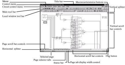
Figure 2-16 The Schematic editor
Menus
Menus, located at the top of the display, select major functions. Circuit windows are used to create or edit circuit schematics or SPICE text files. The Tool bar is used to select modes, tools and other options.
Control menu
The rectangular box in the upper left of the Micro-Cap 6 window is called the Control menu. It can be used to control the window characteristics with the keyboard. It provides these standard Windows options:
Restore: This restores the MC6 window to its former size after it has been enlarged with the Maximize command or reduced to an icon with the Minimize command.
Move: This command lets you move the MC6 window by using the cursor keys. Size: This command lets you resize the MC6 window with the cursor keys. Minimize: This command minimizes the MC6 window to icon size. Maximize: This command maximizes the MC6 window to its maximum size. Close: This command closes the window and exits MC6. ALT + F4 also works. Switch To: This command opens the Task
38