

96 |
POWER EXCEL WITH MR EXCEL |
|
|
|
PARSE MULTI-LINE CELLS |
Problem: Someone used the Alt+Enter trick discussed later in this book to build address information with three lines in single cells. I need to break this data into columns.
Strategy: The Alt+Enter keystroke creates a character code 10. I’ve used many tricks to solve this, including =SUBSTITUTE(A1,CHAR(10),”,”) to change the line feeds to commas. But, the solution is much simpler than this.
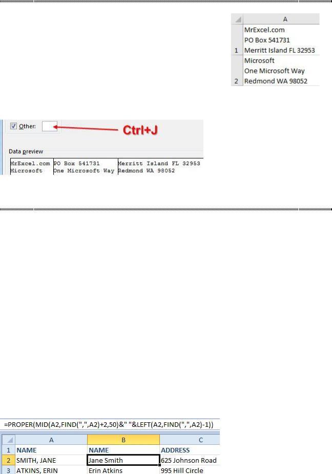
Select the data. Use Data, Text to Columns. In Step 1, choose Delim- ited. In Step 2, choose Other. Click in the Other box and press Ctrl+J.
The data preview will show each line of the cell going to a new column. Apparently, Ctrl+J inserts a character 10 in the Other box.
Figure 230 They used Alt+Enter to enter multi-line data in one cell.
Figure 231 Ctrl+J solves the problem.
CHANGE SMITH, JANE TO JANE SMITH
Problem: I have a column of names in last name, first name style. How can I convert the data to first name last name?
Strategy For Excel 2013: Flash Fill comes to the rescue! Type a heading in B1. Type Jane Smith in B2. Type E in B3. Flash Fill will preview the rest of the column. Press Enter. You are done.
Strategy for Excel 2010: While you could do this in many steps, using Text to Columns and then a concatenation formula, a single large formula would also solve the problem. To begin, you need to insert a blank column after column A to hold the calculation.
=FIND(“,”,A2) will locate the comma within the value in column A. In Smith, Jane, the comma is the sixth character, so the FIND function would return a 6.
The first name starts two characters after the result of the FIND function. It extends to the end of the text. You can use the MID function to isolate the first name. The MID function requires some text, a starting location, and a length. If you ask for more characters than are in the text, then Excel will return from the starting position to the end of the text. For example, if you ask for 50 characters, Excel will handle any first name that has 50 characters or less. Therefore, you use =MID(A2,FIND(“,”,A2)+2,50).
The last name is always the leftmost characters, so you can use =LEFT(A2,FIND(“,”,A2)-1).
To join the first name and last name together, you concatenate the function for the first name, a space in quotes, and the function for the last name. You need to be sure to leave the = sign off the LEFT function because you don’t prefix the function with an equals sign when it occurs in the middle of the formula.
If you want the text in uppercase and lowercase, you need to wrap the entire function in the PROPER function.
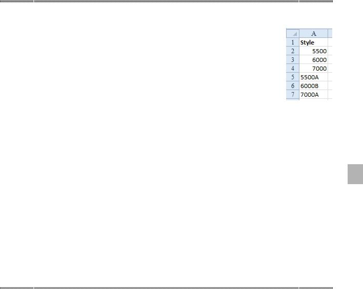
As shown below, the formula is =PROPER(MID(A2,FIND(“,”,A2)+2,50)&” “&LEFT(A2,FIND(“,”,A2)-1)).
Figure 232 The formula in column B achieves the result..
PART 2: CALCULATING WITH EXCEL |
|
97 |
|
|
|
|
CONVERT NUMBERS TO TEXT |
|
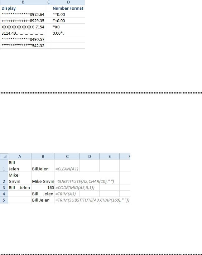
Problem: I have a field that can contain numbers and text. I need the numeric entries to sort with the text entries. However, Excel always sorts the numeric entries to the top of the list, followed by the text entries.
Figure 233 Numbers sort before text that looks like numbers.
Strategy: This is a rare case in which you need to convert numeric entries to text entries.
If you were building this spreadsheet from scratch, you could select column A, select Home, Format, For- mat Cells, and then format the column as text. This would allow all future entries to automatically be converted to text. However, converting cells to have a text format does not retroactively convert numbers to text.
Another option would be to edit each cell that contains a number. To do this, you select the cell, press F2 2 to edit the cell, press Home to move to the beginning of the cell, and type an apostrophe. Then you press
Enter to move to the next cell. This could get very tedious with more than a few cells to change.
The good news is that there is an easier method for converting all the entries in a column to text:
1. Select all the data in a column. Select Data, Text to Columns. In step 1 of the Convert Text to Col- umns Wizard, indicate that your data is fixed width.
2. In step 2 of the wizard, if you have any vertical lines drawn in the Data Preview section, double-click to remove them.
3. In step 3 of the wizard, choose Text as the column data format. 4. Click Finish. The column will be converted to text.
Alternate Strategy: You could also insert a temporary column with the formula =TEXT(A2,“@”).
FILL A CELL WITH REPEATING CHARACTERS
Problem: I need to fill a cell with asterisks before the number. If the cell gets wider, I want more asterisks to appear.
Strategy: Use a custom number format.
Select the cells and press Ctrl+1 (Ctrl and one). Select the Number tab. Choose Number or Currency or whatever style you want for your numbers. Then, in the Category list, choose Custom. You will now be able to edit the custom number format code.
To fill a cell with a character, you enter an asterisk and then that character.
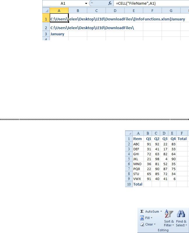
For example, to precede a number with asterisks, you would use **0.00. To precede the number with plus signs, use *+0.00. You can have a number and then fill to the right with a character. Use 0*. to fill with periods.
98 |
POWER EXCEL WITH MR EXCEL |
|
|
Figure 234 Custom number formats fill the cell.
Additional Details: Lotus 1-2-3 used to support using \* in a cell to fill the cell with asterisks. Excel will still support this, but you have to go to File, Options, Advanced, Transition, and choose Transition Navigation Keys. It seems very unlikely that everyone in your department will want to use these settings, so this method is not as reliable as using the custom number format.
CLEAN HASN’T KEPT UP WITH THE TIMES
Problem: The Excel function CLEAN is supposed to get rid of non-printable characters. It doesn’t seem to get them all. And sometimes I would rather replace the non-printable character with a space.
Strategy: CLEAN and TRIM were written a long time ago. The CLEAN function was written in the days when the only characters were 0 through 127. It is designed to remove characters 0 through 31 from data, but it does not touch the new nonprintable characters such as 129, 141, 143, 144, and 157.
The TRIM function removes leading spaces, trailing spaces, and repeated internal spaces. However, it was designed before the advent of the web. TRIM works fine with character 32, but ignores the common character 160 that many web pages use.
You will have better results if you identify the code of the offending character and use =SUBSTITUTE.
Figure 235 Examples of SUBSTITUTE.
In B1 above, CLEAN does successfully remove the Alt+Enter, but it would look better if there were a space instead. The formula shown in C2 solves the problem by replacing CHAR(10) with a space.
In C4, TRIM is not getting rid of the extra interior spaces. The formula shown in C3 uses CODE to identify that those spaces are character 160 instead of regular spaces. The formula shown in C5 uses SUBSTI- TUTE to replace the CHAR(160) with a regular space.
ADD THE WORKSHEET NAME AS A TITLE
Problem: I have 12 worksheets, labeled January through December. Is there a formula that will put a worksheet name in a cell?
Strategy: You can parse the sheet name from the CELL function.
TheCELLfunctioncanreturnavarietyofinformationaboutthetop-leftcellinareference.=CELL(“Col”,A1) will tell you that A1 is in column 1. For this particular problem, =CELL(“FileName”,A1) will return the path, filename, and worksheet name of a saved workbook, as shown in cell A1 below.
PART 2: CALCULATING WITH EXCEL |
99 |
|
|
Figure 236 CELL returns the path, filename and worksheet name. |
|
To isolate the sheet name, you look for the right square bracket by using the FIND function. Then you use |
|
that location plus 1 as the start position for the MID function. |
|
=MID(CELL(“FileName”,A1),FIND(“]”,CELL(“FileName”,A1)+1,25) |
|
returns the worksheet name. Note that the final 25 argument is any number large enough to handle the |
|
longest sheet name you’ve used. |
|
Additional Details: If you need to insert just the worksheet path in a cell, you can use =INFO(“Directory”) |
|
instead of trying to parse it from the CELL function. |
|
Gotcha: The INFO function used to be able to return several bits of information about memory available, |
|
total memory, and so on. These results have not been correct since Windows XP. Today, Excel will return |
|
|
|
#N/A if you use the INFO function to return available memory. |
2 |
|
|
USE AUTOSUM TO QUICKLY ENTER A TOTAL FORMULA
Problem: I have numeric data in Excel. I need to total the rows quickly.
Figure 237 Add total formulas.
Strategy: You can use the AutoSum button on the Home tab or Formulas tab. The AutoSum button is a
Greek letter sigma.
Figure 238 A Greek letter sigma is the math symbol for sum.
Here’s how you use AutoSum to add a total formula: