

52 |
POWER EXCEL WITH MR EXCEL |
|
|
Figure 115 This ribbon tab only appears from Page Layout view.
3. From the Footer dropdown, select Page 1 of ?. Excel will add a footer such as Page 1 of 10 at the bottom of each page.
4. Click outside the header or footer area to close the Header & Footer Tools tab.
Alternate Strategy: You can also build headers and footers the same way as you did in Excel 2003: If you display the Page Layout tab of the ribbon, a small icon (called a dialog launcher) appears in the lower-right corner of the Page Setup group (see Figure 22 on page 12). You click this icon to display the Page Setup dialog, and then you click the Header/Footer tab and make the appropriate settings.
Additional Details: You can also customize left, center, and right headers as you do the footers.
You can specify different footers for the first page and different footers for odd vs. even pages. You control these settings in the Options area of the Header & Footer Tools Design tab of the ribbon.
Gotcha: Sometimes the footer text will crash into the data from the report. If you have adjusted the lower margin to 0.5 inch, you should adjust the footer margin to 0.25 inch to prevent this condition. Use Page
Layout, Margins, Custom Margins to adjust.
Gotcha: Say that you want Sheet1 to be numbered 1 through 10, then Sheet2 to be numbered 11 through 15. Set up each footer to have a page number. When you print, change Print Active Sheets to Print Entire
Workbook. If you only want to print a subset of worksheets, put those worksheets in Group Mode before printing. If you print each sheet separately, the numbers will restart on each worksheet.
HOW TO MAKE A WIDE REPORT FIT TO ONE PAGE WIDE BY MANY PAGES TALL
Problem: After I create a wide report, it prints four pages wide. How do I make it print one page wide?
Figure 116 Taping four pages together leads to copier jams.
Strategy: Ultimately, you will set the Scale to Fit settings to print to one page wide by any number of pages tall. Before you can do that, you should follow these steps:
1. Eliminate extra columns from the print range. Because this worksheet has some lookup tables beyond column X that you do not want to print, highlight columns A through X and select Page Layout,
Print Area, Set Print Area.
2. Set long headings on two lines rather than one. For example, Sales Rep in cell D5 could be on two lines to save width in the column. In cell C5, type Sales, press Alt+Enter, and type Rep. Do the same thing for Prior Year in X5.
3. Make the columns narrower. Select the data in A5:X130 and then select Home, Format, AutoFit
Column Width. Gotcha: The AutoFit command does not deal well with cells in which Alt+Enter was used, as in step 2. You therefore have to manually adjust the column width of columns D and X.
4. Change the orientation to Landscape by selecting Page Layout, Orientation, Landscape.
5. Adjust the margins by selecting Page Layout, Margins, Custom Margins. On the Margins tab of the
Page Setup dialog, set the top, left, and right margins at 0.25 inch. Adjust the bottom to 0.5 inch and
PART 1: THE EXCEL ENVIRONMENT |
53 |
|
|
the footer margin to 0.25 inch. Alternatively, use Print Preview and click the Show Margins icon in the lower right. You can now drag the margins to a new location.
6. On the Page Layout tab, open the Width dropdown in the Scale to Fit group. Choose 1 page. (This is much easier than using the Page Setup dialog, as discussed in the following alternate strategy.)
Results: The report will fit on one page wide and three pages tall.
Alternate Strategy: You can use the Page Layout dialog to indicate that the report should fit to one page wide by <blank> pages tall. On the Page Layout tab of the ribbon, click the dialog launcher in the lower- right corner of the Page Setup group. Choose the Page tab of the Page Setup dialog. Choose Fit To. Leave the first spin button at 1 Page(s) Wide. Using your mouse, highlight the 1 in the spin button for Tall. After the 1 is highlighted, press Delete to leave this entry completely blank. Before Excel 2007, you followed this rather convoluted process to create a setting equivalent to step 6 above.
See Also: "How to Fit a Multiline Heading into One Cell" on page 233.
ADD A PRINTABLE WATERMARK |
1 |
|
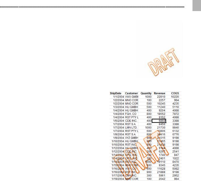
Problem: I would like to add a “Draft” watermark on each page of my printed worksheet.
Strategy: The center header is the gateway to adding a semitransparent watermark image that will print behind your document.
To effectively use this trick, you need to create a graphic that has a fair amount of white space at the top of the picture. The figure below shows a DRAFT stamp at the bottom of some white space. You can create this graphic in Photoshop or any photo- editing tool. I actually created this in Excel as WordArt. On the Page Layout tab, uncheck view Gridlines to create the white space. I then used the free Greenshot utility to capture a region of the screen.
Figure 117 Add whitespace above..
Follow these steps to create the watermark:
1. Select the Page Layout view icon in the bottom-right corner of the Excel window.
2. Click in the Center Header zone at the top of the worksheet. Excel displays the Header & Footer Tools
Design tab.
3. Click the Picture icon on the Header & Footer Tools tab. Browse for and select your picture. Excel inserts
&[Picture] in the header.
If your graphic is too large or small, use the Format Picture icon. You can adjust the size, but not the location. If you need more or less white space, you will have to go back to Photoshop to change the graphic.
This figure shows the resulting graphic drawn in behind your numbers.
Figure 118 The header appears behind your document.
54 |
POWER EXCEL WITH MR EXCEL |
|
|
|
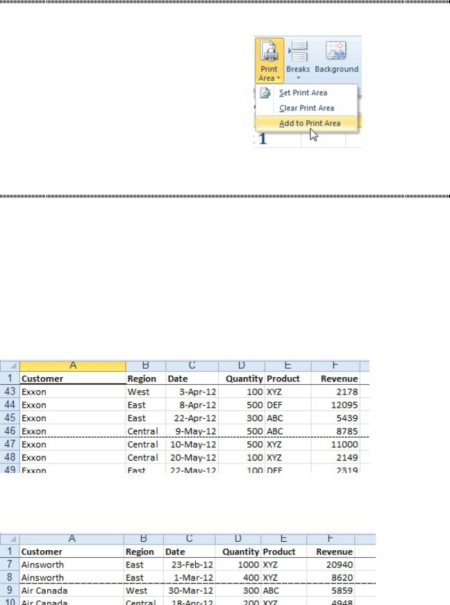
PRINT MULTIPLE RANGES |
Problem: I want to print five sections of my worksheet, but the print areas are not next to each other.
Strategy: Choose the first range to print and use Page |
|
Layout, Print Area, Set Print Area. |
|
Choose the next range to print. This time, a new menu |
|
item is available. Choose Page Layout, Print Area, Add |
|
to Print Area. |
|
You can continue adding additional ranges to the print |
|
area. |
|
Gotcha: Unfortunately, Excel will add a page break be- |
|
tween each section of the print area. |
Figure 119 Add non-adjacent print ranges. |
|
ADD A PAGE BREAK AT EACH CHANGE IN CUSTOMER
Problem: My data is sorted by customer in column A. I want to put each customer on a different page.
Strategy: The easiest way to do this is to add a subtotal by using the Data, Subtotals command. In the Subtotal dialog, you can choose to have a page break between groups. For more about subtotals, see "Add Subtotals to a Data set" on page 249.
However, let’s assume that you cannot use the automatic Subtotals feature for some reason. It helps to understand page breaks.
Excel page breaks can either be automatic or manual. If you access Print Preview and then close Print Preview, Excel will draw in the automatic page breaks.
In this particular report, it turns out that with these margins and print size, Excel would normally offer an automatic page break after row 46. After you do a Print Preview, Excel draws in a dashed line after row 46 to indicate that this is an automatic page break.
Figure 120 The dashed line is an automatic page break.
You can add a manual page break to any row. You position the cell pointer in column A on the first row for a new customer and then select Page Layout, Breaks, Insert Page Break. Excel will draw in a dotted line above the cell pointer to indicate that there is a page break after row 8.
Figure 121 Slightly longer dashes indicate a manual page break.

PART 1: THE EXCEL ENVIRONMENT |
55 |
|
|
Here is a zoomed-in view of the different dashes used for each break. I am not sure the difference will even show up in the book or e-book.
Because you’ve added a manual page break after row 8, Excel will automatically calculate that it can fit |
|
|
rows 9 through 54 on page 2. The location for the next automatic page break is now shown at row 55 in- |
|
|
stead of row 47. |
|
|
Automatic page breaks will move around. Say that you change the margins for the page, using Page Lay- |
|
|
out, Margins. Excel will now calculate that the end of the second page is at another row. |
|
|
1 |
||
Unlike automatic page breaks, manual page break will never move. |
||
|
||
To add the rest of the page breaks, you move the cell pointer to the next cell in column A that has a new |
|
|
customer and select Page Layout, Breaks, Insert Page Break. Because you have 50 of these to insert, you |
|
|
might want to use the keyboard shortcut: Alt+I+B or Alt+P+B+I. |
|
|
Additional Details: Selecting each new customer is tedious. Microsoft provides a shortcut for finding |
|
|
the next cell in the current column that is different from the active cell. However, it is difficult to use this |
|
|
shortcut. You will have to decide if it is worth the hassle. You start with the cell pointer on a customer. |
|
|
Then you press Ctrl+Shift+Down Arrow to select all the cells below the current cell. You press the F5 key |
|
|
and then click the Special button. Finally, you select Column Differences and click OK. The cell pointer |
|
|
will move to the first row that contains a new customer. You can then use the Breaks, Insert Page Break |
|
|
command. You can repeat this whole series of events by holding down the Alt key while you type EGSM. |
|
|
Release the Alt key and press Enter. Hold down the Alt key while you type IB. If you have hundreds of |
|
|
page breaks to add, mastering this keystroke might be worth the time. |
|
|
Additional Details: These steps might be easier than the above. Insert a new column A. The formula |
|
|
in A3 is =IF(B3=B2,1,True). Copy this formula down to all rows. Select column A. Press F5, then click |
|
|
Special. In the Go To Special dialog, choose Formulas. Uncheck Numbers, Text, and Errors, leaving only |
|
|
Logicals selected. Click OK. Do Alt+I+B to insert a break at the first customer. Press Enter to move to the |
|
|
next customer. Press F4 to repeat the last command (insert break). Continue pressing Enter, F4, Enter, |
|
|
F4 until you reach the bottom. You can then delete column A. |
|
|
Additional Details: To remove a manual page break, you should put the cell pointer in the first cell under |
|
|
the manual page break. When the cell pointer is in this location, the Breaks dropdown offers a Remove |
|
|
Page Break option. |
|
|
To remove all page breaks, you select all cells by using the box to the left of column A. The Breaks drop- |
|
|
down will now offer the option Reset All Page Breaks. |
|
|
Gotcha: To insert a row page break, you must either select the entire row or have the cell pointer in col- |
|
|
umn A. If you select Insert Page Break while in cell C9, Excel will insert a horizontal page break above row |
|
|
9 and also a vertical page break to the left of column C. This is rarely what you want. |
|
SAVE MY WORKSHEET AS A PDF FILE
Problem: I want to send my worksheet to a high-level manager, but I don’t want him screwing around with the formulas. Can I send it as a PDF file?
Excel will let you save your workbooks as PDF files. In Excel 2013, use File, Export, Create PDF/XPS.)
Think of Saving as PDF as if you are printing the workbook to a PDF file. In the Publish as PDF or XPS dialog, you can click the Options button to control if you want the selection, active sheets, or entire work- book sent to the PDF file.