


Author
V. Ganapathy is a consultant on steam generators and waste heat boilers based in Chennai, India. He has over 40 years of experience in the engineering of steam generators and waste heat boilers with emphasis on thermal design, performance, and heat transfer aspects. He also develops custom software on boiler design and performance. He holds a bachelor’s degree in mechanical engineering from IIT Madras and an MSc (Engg.) from Madras University.
Ganapathy has published over 250 articles on steam generators and thermal design and has authored five books on boilers, the latest being Industrial Boilers and HRSGs (Taylor & Francis Group, Boca Raton, Florida). He also conducts intensive courses on boilers for chemical plants, refineries, and engineering consulting companies worldwide.
He has contributed several chapters to the Handbook of Engineering Calculations (McGraw Hill), Encyclopedia of Chemical Processing and Design (Marcel Dekker, New York), and recently a chapter on HRSG to the book Power Plant Life Management and Performance Improvement
(Woodhouse Publishing, United Kingdom).
xxxi

1
Combustion Calculations
Introduction
Boiler combustion and efficiency calculations are the starting point for boiler performance evaluation. These calculations enable the boiler designer or the plant engineer to estimate the boiler efficiency, air quantity required for combustion, and flue gas quantity generated in a boiler or heater; flue gas analysis that impacts convective and nonluminous heat transfer coefficients, adiabatic combustion temperature, flue gas specific heat, and enthalpy is also obtained from combustion calculations; these data in turn aid furnace performance evaluation, sizing, or performance evaluation of heat transfer equipment in the gas path, help evaluate airand gas-side pressure drops, and also estimate the water and acid dew point temperatures. CO, NOx, and CO2 emission conversion calculations also require that results of combustion calculations are available. If NOx emission is to be limited, then one has to estimate the amount of flue gas recirculation (FGR) to dampen the combustion temperature that impacts NOx formation. Thus, basic and useful information for boiler performance evaluation can be generated from combustion calculations. The emphasis in this chapter is on oil and gaseous fuels. Sometimes, multiple fuels are fired in a boiler simultaneously, and this issue is also discussed.
Moisture in Air
Air is required for the combustion of fossil fuels. However, atmospheric air is never dry. It contains a certain amount of moisture due to local humidity and ambient temperature conditions. This adds to the volume of air to be handled by the forced draft fan and also increases the amount of water vapor in the flue gas. The amount of moisture in air may be obtained using psychometric chart (Figure 1.1) or estimated from the equation [1]:
M = 0.622Pw/(1.033 – Pw) |
(1.1) |
where Pw is the partial pressure of water vapor in air, kg/cm2 a. For example, at 27°C, from steam tables, the saturated vapor pressure is 0.5069 psia = 0.0356 kg/cm2 a, and if the relative humidity is say 65%, then
Pw = 0.65 × 0.0356 = 0.0231 kg/cm2 a
1

2 |
Steam Generators and Waste Heat Boilers: For Process and Plant Engineers |
|
0.028 |
|
|
|
|
|
|
|
|
|
|
|
|
|
|
|
|
|
Psychrometric chart |
|
|
|
85 |
|
|
|
|
90 |
|||
|
0.024 |
|
|
|
|
|
|
|
|
|
|
|
|
||
|
Relative humidity = |
|
|
|
|
|
|
|
|
|
|
|
|
||
|
|
|
|
|
|
|
|
|
|
|
|
|
|
||
|
|
Mole fraction of H2O vapor in moist air |
100 |
|
80 |
|
|
|
|
|
|||||
|
|
|
Mole fraction at saturation |
|
|
|
|
|
|
|
|||||
|
0.020 |
|
|
|
80 |
|
|
|
|
|
|||||
|
|
|
|
|
|
|
|
|
|
|
|
|
|
||
air |
|
|
|
|
|
|
|
|
75 |
60 |
50 |
|
|
|
|
|
|
|
|
|
|
|
|
We |
|
40 |
|
|
|||
|
|
|
|
|
d air |
|
|
|
|
|
|
||||
dry |
|
|
|
|
|
|
|
|
|
|
|
|
|||
0.016 |
|
|
|
|
|
|
|
t |
|
|
|
|
|||
|
|
|
|
70 |
|
|
-bulb |
temp |
|
|
|||||
water/lb |
|
|
|
|
|
turate |
|
|
|
erature, |
30 |
|
|||
|
|
|
|
|
|
|
|
|
|
||||||
|
|
|
|
Sa |
|
|
|
|
|
|
|
||||
|
|
|
|
|
|
|
|
|
|
|
20 |
||||
0.012 |
|
|
|
65 |
|
|
|
|
|
|
°F |
||||
|
|
|
|
|
|
|
|
|
|
||||||
|
|
|
|
|
|
|
|
|
|
|
|||||
Lb |
|
|
|
|
|
60 |
|
|
|
|
|
|
|
|
|
|
|
|
|
|
|
|
|
|
|
|
|
|
|
|
|
|
0.008 |
|
|
55 |
|
|
|
|
|
|
|
|
% |
|
|
|
|
|
50 |
|
|
|
|
|
|
|
|
|
|
||
|
|
|
|
|
|
|
|
humidity |
|
|
|||||
|
|
|
45 |
|
|
|
|
|
|
10 |
|||||
|
|
|
|
|
|
|
|
|
|
||||||
|
|
|
|
|
|
|
|
|
Relative |
|
|
|
|
||
|
0.004 |
32 |
40 |
|
|
|
|
|
|
|
|
|
|
|
|
|
|
|
|
|
|
|
|
|
|
|
|
|
|||
|
|
|
|
|
|
|
|
|
|
|
|
|
|
||
|
|
|
|
|
|
|
|
|
|
|
|
|
|
|
|
|
0.000 |
40 |
50 |
60 |
|
70 |
|
80 |
|
90 |
|
100 |
110 |
120 |
|
|
30 |
|
|
|
|
||||||||||
Dry-bulb temperature, °F
FIGURE 1.1
Moisture in air due to relative humidity.
Hence, M = 0.622 × 0.0231/(1.033 – 0.0231) = 0.0142 kg/kg air or 0.0142 lb/lb air. If 1000 kg of dry air is required for combustion in a boiler, the actual wet air that should be sent to the burner will be 1014.2 kg, and the boiler fan has to be sized for the volume of this amount of wet air.
Combustion Calculations
Knowing the fuel analysis, excess air, and ambient conditions, one may perform combustion calculations as shown in the following text.
Example 1.1
Natural gas having CH4 = 83.4%, C2H6 = 15.8%, and N2 = 0.8 by volume is fired in a boiler using 15% excess air. Ambient temperature is 20°C and relative humidity is 80%. Perform combustion calculations and determine the flue gas analysis.
Solution
From steam tables, the saturated vapor pressure at 20°C (68°F) is 0.34 psia = 0.0239 kg/cm2 a. At 80% relative humidity, Pw = 0.8 × 0.0239 = 0.0191 kg/cm2 a
Combustion Calculations |
3 |
M = .622 × 0.0191/(1.033 – 0.0191) = 0.012 (same information may be obtained from Figure 1.1). Combustion of methane may be expressed as CH4 +2O2 = CO2 + 2H2O or 1 mol of CH4 requires 2 mol (volumes) of O2 or 2 × 100/21 = 9.53 mol of air for combustion (air contains 21% volume of oxygen and rest nitrogen). Similarly,
2C2H6+ 7O2 = 4CO2 + 6H2O or 1 mol of ethane requires 3.5 mol of O2 or 3.5 × 100/21 = 16.68 mol of dry air for combustion.
Tables 1.1 and 1.2, which give the air required for theoretical combustion of various fuel constituents, may also be used to arrive at these values.
Hence, 100 mol of fuel requires 83.4 × 9.53 + 15.8 × 16.68 = 1058.3 mol of theoretical dry air. Considering 15% excess air factor, actual dry air required = 1.15 × 1058.3 = 1217 mol. Excess air = 0.15 × 1058.3 = 158.7 mol; excess O2 = 158.7 × 0.21 = 33.3 moles and N2 formed = 0.79 × 1217 = 961 mol; air moisture = 1217 × 28.84 × 0.012/18 = 23.5 mol. (We multiplied moles by molecular weight [MW] to get the weight and then converted the moisture in air to volume basis by dividing by the MW of water vapor; here 28.84 is the MW of air and 18 that of water vapor.)
Tables 1.1 and 1.2 may also be used to get the amount of CO2, H2O, and N2 formed. For example, 1 mol of methane forms one mole of CO2. One mole of ethane forms two moles of CO2. Similarly, 1 mol of CH4 forms 2 mol of H2O, and 1 mol of ethane forms 3 mol of H2O. Hence, total amount of CO2 and H2O formed is
CO2 = 83.4 × 1 + 2 × 15.8 = 115 mol;
H2O = 2 × 83.4 + 3 × 15.8 + 23.5 = 237.7 mol (23.5 mol is the air moisture); N2 = 961+0.8 (fuel nitrogen) = 961.8 mol;
O2 (excess) = 33.3 mol
Total moles of flue gas formed = 115 + 237.7 + 961.8 + 33.3 = 1347.8 mol
Flue Gas Analysis and Air–Flue Gas Quantities
%volume CO2 in flue gases = (115/1347.8) × 100 = 8.5%
%volume H2O = (237.7/1347.8) × 100 = 17.7%
N2 = (961.8/1347.8) × 100 = 71.36% % O2 = (33.3/1347.8) × 100 = 2.47%.
This analysis is on wet basis. To convert to dry basis, one has to subtract the water content and recalculate the analysis. (Dry analysis is required as some instruments measure the oxygen content on dry basis from which excess air is computed.)
On dry basis, CO2 = 8.5 × 100/(100 – 17.7) = 10.3%, O2 = 2.47 × 100/(100 – 17.7) = 3%, and N2 = 71.36 × 100/(100 – 17.7) = 86.7%. For efficiency calculations, one has to know the dry and wet air quantities and dry and wet flue gas formed per kg of fuel. See Table 1.3.
For nonluminous heat transfer calculations, one requires the partial pressures of CO2 and H2O. pw = 237.7/1347.8 = 0.176 atm and pc = 115/1347.8 = 0.085 atm.
MW of flue gas = 8.5 × 44 + 17.7 × 18 + 71.36 × 28 + 2.47 × 32 = 27.70.
CO2 on mass basis in flue gas is required for emission calculations as it is considered a pollutant. % weight of CO2 in flue gas = 8.5 × 44/27.7 = 13.5. One may also compute the emissions of CO2/million J of heat input.
Amount of fuel fired per million J of energy input on higher heating value (HHV) basis = 106/ (53.940 × 10⁶) = 0.01854 kg fuel. (HHV of the fuel is 53,940 kJ/kg [or 53.94 × 10⁶ J/kg] as shown later.) Hence, CO2 formed = 20.4 × 0.01854 × 0.135 = 0.051 kg/MM J.
Per MM Btu (1054 MM J), the CO2 emissions = 1054 × 0.051 = 53.75 kg (118.5 lb). (20.4 is the quantity of wet flue gas produced, kg/kg fuel, see Table 1.3.)

TABLE 1.1
Combustion Constants (Part 1)
|
|
|
|
|
|
|
|
|
|
|
Heat of Combustionc |
|
||
|
|
|
|
|
|
|
|
|
|
Btu/cu ft |
Btu/lb |
|||
No. |
Substance |
|
Formula |
Mol. Wta |
Lb per cu ftb |
Cu ft per lbb |
|
Sp. gr. Air = 1000b |
|
|
|
|
|
|
|
|
Gross |
Netd |
Gross |
Netd |
|||||||||
1 |
Carbon |
|
C |
|
12.01 |
— |
— |
|
— |
— |
— |
14,093g |
14,093 |
|
2 |
Hydrogen |
|
H2 |
|
2.016 |
0.005327 |
187.723 |
0.06959 |
325.0 |
275.0 |
61,100 |
51,623 |
||
3 |
Oxygen |
|
O2 |
|
32.000 |
0.08461 |
11.819 |
1.1053 |
— |
— |
— |
— |
||
4 |
Nitrogen (atm.) |
|
N |
|
28.016 |
0.07439c |
13.443c |
|
0.9718e |
— |
— |
— |
— |
|
|
|
2 |
|
|
|
|
|
|
|
|
|
|
|
|
5 |
Carbon monoxide |
|
C2O |
|
28.01 |
0.07404 |
13.506 |
0.9672 |
321.8 |
321.8 |
4,347 |
4,347 |
||
6 |
Carbon dioxide |
|
CO2 |
|
44.01 |
0.1170 |
8.548 |
1.5282 |
— |
— |
— |
— |
||
Paraffin series CnH2n+2 |
|
|
|
|
|
|
|
|
|
|
|
|
|
|
7 |
Methane |
|
CH4 |
|
16.041 |
0.04243 |
23.565 |
0.5543 |
1013.2 |
913.1 |
23,879 |
21,520 |
||
8 |
Ethane |
|
C H |
6 |
30.067 |
0.08029c |
12.455c |
|
1.04882e |
1792 |
1641 |
|
22,320 |
20,432 |
|
|
2 |
|
|
|
|
|
|
|
|
|
|
||
9 |
Propane |
|
C H |
8 |
44.092 |
0.1196c |
8.365c |
|
1.5617c |
2590 |
2385 |
|
21,661 |
19,944 |
|
|
3 |
|
|
|
|
|
|
|
|
|
|
||
10 |
n-Butane |
|
C H |
10 |
58.118 |
0.1582c |
6.321c |
|
2.06654e |
3370 |
3113 |
|
21,308 |
19,680 |
|
|
4 |
|
|
|
|
|
|
|
|
|
|
||
11 |
Isobutane |
|
C H |
10 |
58.118 |
0.1582e |
6.321e |
|
2.06654e |
3363 |
3105 |
|
21,257 |
19,629 |
|
|
4 |
|
|
|
|
|
|
|
|
|
|
||
12 |
n-Pentane |
|
C H |
12 |
72.144 |
0.1904e |
5.252e |
|
2.4872c |
4016 |
3709 |
|
21,091 |
19,517 |
|
|
5 |
|
|
|
|
|
|
|
|
|
|
||
13 |
Isopentane |
|
C H |
12 |
72.144 |
0.1904e |
5.252e |
|
2.4872e |
4008 |
3716 |
|
21,052 |
19,478 |
|
|
5 |
|
|
|
|
|
|
|
|
|
|
||
14 |
Neopentane |
|
C H |
12 |
72.144 |
0.1904e |
5.252e |
|
2.4872e |
3993 |
3693 |
|
20,970 |
19,396 |
|
|
5 |
|
|
|
|
|
|
|
|
|
|
||
15 |
n-Hexane |
|
C H |
14 |
86.169 |
0.2274e |
4.398e |
|
2.9704c |
4762 |
4412 |
|
20,940 |
19,403 |
|
|
6 |
|
|
|
|
|
|
|
|
|
|
||
Olefin series CnH2n |
|
|
|
|
|
|
|
|
|
|
|
|
|
|
16 |
Ethylene |
|
C2H4 |
28.051 |
0.07456 |
13.412 |
0.9740 |
1613.8 |
1513.2 |
21,644 |
20,295 |
|||
17 |
Propylene |
|
C H |
6 |
42.077 |
0.1110e |
9.007e |
|
1.4504e |
2336 |
2186 |
|
21,041 |
19,691 |
|
|
3 |
|
|
|
|
|
|
|
|
|
|
||
18 |
n-Butene (butylene) |
|
C H |
8 |
56.102 |
0.1480e |
6.756e |
|
1.9336e |
3084 |
2885 |
|
20,840 |
19,496 |
|
|
4 |
|
|
|
|
|
|
|
|
|
|
||
19 |
Isobutene |
|
C H |
8 |
56.102 |
0.1480e |
6.756e |
|
1.9336e |
3068 |
2869 |
|
20,730 |
19,382 |
|
|
4 |
|
|
|
|
|
|
|
|
|
|
||
20 |
n-Pentene |
|
C H |
10 |
70.128 |
0.1852e |
5.400e |
|
2.4190e |
3836 |
3586 |
|
20,712 |
19,363 |
|
|
5 |
|
|
|
|
|
|
|
|
|
|
||
4
Engineers Plant and Process For Boilers: Heat Waste and Generators Steam

Aromatic series CnH2n–6 |
|
|
|
|
|
|
|
|
|
|
|
|
|
21 |
Benzene |
C H |
6 |
|
76.107 |
0.2060c |
4.852c |
2.6920e |
3751 |
3601 |
18,210 |
17,480 |
|
|
|
6 |
|
|
|
|
|
|
|
|
|
|
|
22 |
Toluene |
C H |
8 |
|
92.132 |
0.2431c |
4.113e |
3.1760e |
4484 |
4284 |
18,440 |
17,620 |
|
|
|
7 |
|
|
|
|
|
|
|
|
|
|
|
23 |
Xylene |
C H |
10 |
106.158 |
0.2803e |
3.567e |
3.6618e |
5230 |
4980 |
18,650 |
17,760 |
||
|
|
8 |
|
|
|
|
|
|
|
|
|
||
Miscellaneous gases |
|
|
|
|
|
|
|
|
|
|
|
|
|
24 |
Acetylene |
C2H2 |
|
26.036 |
0.06971 |
14.344 |
0.9107 |
1499 |
1448 |
21,500 |
20,776 |
||
25 |
Naphthalene |
C H |
8 |
128.162 |
0.3384e |
2.955e |
4.4208e |
5854f |
5654f |
17,298f |
16,708f |
||
|
|
10 |
|
|
|
|
|
|
|
|
|
|
|
26 |
Methyl alcohol |
CH OH |
32.041 |
0.0846e |
11.820e |
1.1052e |
867.9 |
768.0 |
10,259 |
9,078 |
|||
|
|
3 |
|
|
|
|
|
|
|
|
|
|
|
27 |
Ethyl alcohol |
C H |
5 |
OH |
46.067 |
0.1216e |
8.221e |
1.5890e |
1600.3 |
1450.5 |
13,161 |
11,929 |
|
|
|
2 |
|
|
|
|
|
|
|
|
|
|
|
28 |
Ammonia |
NH |
3 |
|
17.031 |
0.0456e |
21.914e |
0.5961e |
441.1 |
365.1 |
9,668 |
8,001 |
|
29 |
Sulfur |
S |
|
|
|
32.06 |
— |
— |
— |
— |
— |
3,983 |
3,983 |
30 |
Hydrogen sulfide |
H S |
|
|
|
34.076 |
0.09109e |
10.979e |
1.1898e |
647 |
596 |
7,100 |
6,545 |
|
|
2 |
|
|
|
|
|
|
|
|
|
|
|
31 |
Sulfur dioxide |
SO2 |
|
|
|
64.06 |
0.1733 |
5.770 |
2.264 |
— |
— |
— |
— |
32 |
Water vapor |
H O |
|
18.016 |
0.04758e |
21.017e |
0.6215e |
— |
— |
— |
— |
||
|
|
2 |
|
|
|
|
|
|
|
|
|
|
|
33 |
Air |
— |
26.9 |
0.07655 |
13.063 |
1.0000 |
— |
— |
— |
— |
|||
Source: Ganapathy, V., Industrial Boilers and HRSGs, CRC Press, Boca Raton, FL, 2003, p238.
All gas volumes corrected to 60°F and 30 in. Hg dry. For gases saturated with water at 60°F, 1.73% of the Btu value must be deducted.
aCalculated from atomic weights given in the Journal of the American Chemical Society, February 1937.
bDensities calculated from values given in gL at 0°C and 760 mmHg in the International Critical Tables allowing for the known deviations from the gas laws. Where the coefficient of expansion was not available, the assumed value was taken as 0.0037 per 0°C. Compare this with 0.003662, which is the coefficient for a perfect gas. Where no densities were available, the volume of the mole was taken as 22.4115 L.
cConverted to mean Btu per lb (1/180 of the heat per lb of water from 32°F to 2120°F) from data by Frederick D. Rossini, National Bureau of Standards, letter of April 10, 1937, except as noted.
dDeduction from gross to net heating value determined by deducting 18,919 Btu/lb mol water in the products of combustion. Osborne, Stimson, and Ginnings, Mechanical Engineering, p. 163, March 1935, and Osborne, Stimson, and Flock, National Bureau of Standards Research Paper 209.
eDenotes that either the density or the coefficient of expansion has been assumed. Some of the materials cannot exist as gases at 60°F and 30 in. Hg pressure, in which case the values are theoretical ones given for ease of calculation of gas problems. Under the actual concentrations in which these materials are present, their partial pressure is low enough to keep them as gases.
fFrom third edition of Combustion.
Calculations Combustion
5

TABLE 1.2
Combustion Constants (Part 2)
|
|
Cu ft per cu ft of Combustible |
|
|
|
|
|
|
|
|
Lb per lb of Combustible |
|
|
||||||||
|
|
|
|
|
|
|
|
|
|
|
|
|
|
|
|
||||||
|
|
|
|
|
|
|
|
|
|
|
|
|
|
|
|||||||
|
Required for Combustion |
|
|
|
|
Flue Products |
Required for Combustion |
|
Flue Products |
Experimental Error |
|
||||||||||
|
|
|
|
|
|
|
|
|
|
|
|
|
|
|
|
|
|
|
|
|
|
No. |
Substance |
O2 |
N2 |
Air |
CO2 |
H2O |
N2 |
|
O2 |
N2 |
Air |
CO2 |
H2O |
N2 |
in Heat of (±%) |
|
|||||
|
|
|
|
|
|
|
|
|
|
|
|
|
|
|
|
|
|
|
|
|
|
1 |
Carbon |
— |
— |
— |
— |
— |
— |
2.664 |
8.863 |
11.527 |
3.664 |
— |
8.863 |
0.012 |
|
||||||
2 |
Hydrogen |
0.5 |
1.882 |
2.382 |
|
— |
1.0 |
1.882 |
7.937 |
26.407 |
34.344 |
— |
8.937 |
26.407 |
0.015 |
|
|||||
3 |
Oxygen |
— |
— |
— |
— |
— |
— |
|
— |
— |
— |
— |
— |
— |
— |
|
|||||
4 |
Nitrogen (atm.) |
— |
— |
— |
— |
— |
— |
|
— |
— |
— |
— |
— |
— |
— |
|
|||||
5 |
Carbon monoxide |
0.5 |
1.882 |
0.2382 |
1.0 |
— |
1.882 |
0.571 |
1.900 |
2.471 |
1.571 |
— |
1.900 |
0.045 |
|
||||||
6 |
Carbon dioxide |
— |
— |
— |
— |
— |
— |
|
— |
— |
— |
— |
— |
— |
— |
|
|||||
Paraffin series CnH2n+2 |
|
|
|
|
|
|
|
|
|
|
|
|
|
|
|
|
|
|
|
|
|
7 |
Methane |
2.0 |
7.528 |
9.528 |
|
1.0 |
2.0 |
7.528 |
3.990 |
13.275 |
17.265 |
2.744 |
2.246 |
13.275 |
0.033 |
|
|||||
8 |
Ethane |
3.5 |
13.175 |
16.675 |
|
2.0 |
3.0 |
13.175 |
3.725 |
12.394 |
16.119 |
2.927 |
1.798 |
12.394 |
0.030 |
|
|||||
9 |
Propane |
5.0 |
18.821 |
23.821 |
|
3.0 |
4.0 |
18.821 |
3.629 |
12.074 |
15.703 |
2.994 |
1.634 |
12.074 |
0.023 |
|
|||||
10 |
n-Butane |
6.5 |
24.467 |
30.967 |
|
4.0 |
5.0 |
24.467 |
3.579 |
11.908 |
15.487 |
3.029 |
1.550 |
11.908 |
0.022 |
|
|||||
11 |
Isobutane |
6.5 |
24.467 |
30.967 |
|
4.0 |
5.0 |
24.467 |
3.579 |
11.908 |
15.487 |
3.029 |
1.550 |
11.908 |
0.019 |
|
|||||
12 |
n-Pentane |
8.0 |
30.114 |
38.114 |
|
5.0 |
6.0 |
30.114 |
3.548 |
11.805 |
15.353 |
3.050 |
1.498 |
11.805 |
0.025 |
|
|||||
13 |
Isopentane |
8.0 |
30.114 |
38.114 |
|
5.0 |
6.0 |
30.114 |
3.548 |
11.805 |
15.353 |
3.050 |
1.498 |
11.805 |
0.071 |
|
|||||
14 |
Neopentane |
8.0 |
30.114 |
38.114 |
|
5.0 |
6.0 |
30.114 |
3.548 |
11.805 |
15.353 |
3.050 |
1.498 |
11.805 |
0.11 |
|
|||||
15 |
n-Hexane |
9.5 |
35.760 |
45.260 |
|
6.0 |
7.0 |
35.760 |
3.528 |
11.738 |
15.266 |
3.064 |
1.464 |
11.738 |
0.05 |
|
|||||
Olefin series CnH2n |
|
|
|
|
|
|
|
|
|
|
|
|
|
|
|
|
|
|
|
|
|
16 |
Ethylene |
3.0 |
11.293 |
14.293 |
|
2.0 |
2.0 |
11.293 |
3.422 |
11.385 |
14.807 |
3.138 |
1.285 |
11.385 |
0.021 |
|
|||||
17 |
Propylene |
4.5 |
16.939 |
21.439 |
|
3.0 |
3.0 |
16.939 |
3.422 |
11.385 |
14.807 |
3.138 |
1.285 |
11.385 |
0.031 |
|
|||||
18 |
n-Butene (butylene) |
6.0 |
22.585 |
28.585 |
|
4.0 |
4.0 |
22.585 |
3.422 |
11.385 |
14.807 |
3.138 |
1.285 |
11.385 |
0.031 |
|
|||||
19 |
Isobutene |
6.0 |
22.585 |
28.585 |
|
4.0 |
4.0 |
22.585 |
3.422 |
11.385 |
14.807 |
3.138 |
1.285 |
11.385 |
0.031 |
|
|||||
20 |
n-Pentene |
7.5 |
28.232 |
35.732 |
|
5.0 |
5.0 |
28.232 |
3.422 |
11.385 |
14.807 |
3.138 |
1.285 |
11.385 |
0.037 |
|
|||||
6
Engineers Plant and Process For Boilers: Heat Waste and Generators Steam
Aromatic series CnH2n–6 |
|
|
|
|
|
|
|
|
|
|
|
|
|
|
21 |
Benzene |
7.5 |
28.232 |
35.732 |
6.0 |
3.0 |
28.232 |
3.073 |
10.224 |
13.297 |
3.381 |
0.692 |
10.224 |
0.12 |
22 |
Toluene |
9.0 |
33.878 |
32.878 |
7.0 |
4.0 |
33.878 |
3.126 |
10.401 |
13.527 |
3.344 |
0.782 |
10.401 |
0.21 |
23 |
Xylene |
10.5 |
39.524 |
50.024 |
8.0 |
5.0 |
39.524 |
3.165 |
10.530 |
13.695 |
3.317 |
0.849 |
10.530 |
0.36 |
Miscellaneous gases |
|
|
|
|
|
|
|
|
|
|
|
|
|
|
24 |
Acetylene |
2.5 |
9.411 |
11.911 |
2.0 |
1.0 |
9.411 |
3.073 |
10.224 |
13.297 |
3.381 |
0.692 |
10.224 |
0.16 |
25 |
Naphthalene |
12.0 |
45.170 |
57.170 |
10.0 |
4.0 |
45.170 |
2.996 |
9.968 |
12.964 |
3.434 |
0.562 |
9.968 |
— |
26 |
Methyl alcohol |
1.5 |
5.646 |
7.146 |
1.0 |
2.0 |
5.646 |
1.498 |
4.984 |
6.482 |
1.374 |
1.125 |
4.984 |
0.027 |
27 |
Ethyl alcohol |
3.0 |
11.293 |
14.293 |
2.0 |
3.0 |
11.293 |
2.084 |
6.934 |
9.018 |
1.922 |
1.170 |
6.934 |
0.030 |
28 |
Ammonia |
0.75 |
2.823 |
3.573 |
— |
1.5 |
3.323 |
1.409 |
4.688 |
6.097 |
— |
1.587 |
5.511 |
0.088 |
|
|
— |
— |
— |
— — |
— |
— |
— |
— |
SO2 |
— |
— |
— |
|
29 |
Sulfur |
— |
— |
— |
— |
— |
— |
0.998 |
3.287 |
4.285 |
1.9928 |
— |
3.287 |
0.071 |
|
|
— |
— |
— |
SO2 |
— |
— |
— |
— |
— |
SO2 |
— |
— |
— |
30 |
Hydrogen sulfide |
1.5 |
5.646 |
7.146 |
1.0 |
1.0 |
5.646 |
1.409 |
4.688 |
6.097 |
1.880 |
0.529 |
4.688 |
0.30 |
31 |
Sulfur dioxide |
— |
— |
— |
— |
— |
— |
— |
— |
— |
— |
— |
— |
— |
32 |
Water vapor |
— |
— |
— |
— |
— |
— |
— |
— |
— |
— |
— |
— |
— |
33 |
Air |
— |
— |
— |
— |
— |
— |
— |
— |
— |
— |
— |
— |
— |
Source: Ganapathy, V., Industrial Boilers and HRSGs, CRC Press, Boca Raton, FL, 2003, p238.
All gas volumes corrected to 60°F and 30 in. Hg dry. For gases saturated with water at 60°F, 1.73% of the Btu value must be deducted.
aCalculated from atomic weights given in the Journal of the American Chemical Society, February 1937.
bDensities calculated from values given in gL at 0°C and 760 mmHg in the International Critical Tables allowing for the known deviations from the gas laws. Where the coefficient of expansion was not available, the assumed value was taken as 0.0037 per 0°C. Compare this with 0.003662, which is the coefficient for a perfect gas. Where no densities were available, the volume of the mole was taken as 22.4115 L.
cConverted to mean Btu per lb (1/180 of the heat per lb of water from 32°F to 2120°F) from data by Frederick D. Rossini, National Bureau of Standards, letter of April 10, 1937, except as noted.
dDeduction from gross to net heating value determined by deducting 18,919 Btu/lb mol water in the products of combustion. Osborne, Stimson, and Ginnings, Mechanical Engineering, p. 163, March 1935, and Osborne, Stimson, and Flock, National Bureau of Standards Research Paper 209.
eDenotes that either the density or the coefficient of expansion has been assumed. Some of the materials cannot exist as gases at 60°F and 30 in. Hg pressure, in which case the values are theoretical ones given for ease of calculation of gas problems. Under the actual concentrations in which these materials are present, their partial pressure is low enough to keep them as gases.
fFrom third edition of Combustion.
Calculations Combustion
7
8 |
Steam Generators and Waste Heat Boilers: For Process and Plant Engineers |
|||
|
TABLE 1.3 |
|
|
|
|
Dry and Wet Flue Gas Analysis |
|
|
|
|
|
|
|
|
|
Basis |
Wet |
Dry |
|
|
|
|
|
|
|
% volume CO2 |
8.5 |
10.3 |
|
|
H2O |
17.64 |
0 |
|
|
N2 |
71.36 |
86.7 |
|
|
O2 |
2.47 |
3.0 |
|
Molecular weight of the fuel = (83.4 × 16 + 15.8 × 30 + 0.8 × 28)/100 = 18.3. wda = kg dry air/kg fuel = 1217 × 28.84/1830 = 19.18.
wwa = kg wet air/kg fuel = 19.18 + 23.5 × 18/1830 = 19.41.
wdg = kg dry flue gas/kg fuel = (115 × 44+33.3 × 32 + 961 × 28)/1830 = 18. wwg = kg wet flue gas/kg fuel = (115 × 44+33.3 × 32 + 961.8 × 28 + 237.7
× 18)/1830 = 20.4.
Water Formed per kg of Fuel
This is an important piece of information as it gives an idea of how much water can be condensed in a condensing economizer if used. In the earlier example, the MW of flue gas = 27.7. The % weight of H2O in the flue gas = 17.64 × 18/27.7 = 11.46. It was shown earlier that wwg = amount of wet flue gas formed per kg of fuel = 20.4. Hence, the amount of water vapor formed per kg fuel fired = 0.1146 × 20.4 = 2.34 kg. Typically, for natural gas, it varies from 2.15 to 2.4. Similar calculations may be carried out for fuel oil. For no. 2 fuel oil at 15% excess air, it can be shown that % volume CO2 = 11.57, H2O = 12.29, N2 = 73.63, O2 = 2.51. MW of flue gas = 11.57 × 44 + 12.29 × 18 + 73.63 × 28 + 2.51 × 32 = 28.72.% weight of H2O in flue gas = 12.29 × 18/28.72 = 7.7%. The amount of flue gas produced per kg fuel is about 18. Hence, 0.077 × 18 = 1.39 kg of water vapor is produced per kg of fuel fired at 15% excess air. On an average, it varies from 1.3 to 1.5 kg/kg fuel, much smaller than that for natural gas. Hence, more energy can be recovered in latent heat form with flue gas from combustion of natural gas than with fuel oils.
Excess Air from Flue Gas Analysis
In operating plants, data on flue gas analysis will be available using which the plant engineer may arrive at the excess air used. This will help the plant engineer evaluate the boiler efficiency, and air and flue gas quantities. A formula that is widely used to obtain excess air E in % is [2]
E = 100 × (O2 – CO/2)/[0.264N2 – (O2 – CO/2)] |
(1.2) |
where O2, CO, and N2 are % volume of oxygen, carbon monoxide, and nitrogen on dry flue gas basis. Another formula is used when an Orsat-type analyzer is used for analyzing the flue gases; SO2 will be absorbed with CO2. The oxygen is on dry volumetric basis.
E = K1O2/(21 – O2) |
(1.3) |
Constant K1 = (100C + 237H2 + 37.5S + 9N2 – 29.6O2)/(C + 3H2 + 0.375S – 0.375O2) |
(1.4) |
where C, H2, N2, S, and O2 are fraction by weight of carbon, hydrogen, nitrogen, sulfur, and oxygen in fuel.

Combustion Calculations |
9 |
Let us check the value of constant K1 for Example 1.1.
%weight of CH4 in fuel = 83.4 × 16/(83.4 × 16 + 15.8 × 30 + 0.8 × 28) = 0.729.
%weight of C2H6 in fuel = 15.8 × 30/(83.4 × 16 + 15.8 × 30 + 0.8 × 28) = 0.259
%N2 by weight in fuel = 0.012
Carbon C in CH4 = 0.75 × 0.729 = 0.5467 and fraction hydrogen = 0.1823 Carbon in C2H6 = (24/30) × 0.259 = 0.2072 and fraction hydrogen = 0.0518
Total C fraction by weight = 0.5467 + 0.2072 = 0.7539, and total hydrogen by weight = 0.0518 + 0.1823 = 0.2341. Hence,
K1 = [100 × 0.7539 + 237 × 0.2341 + 9 × 0.012]/[0.7539 + 3 × 0.2341] = 89.9
Let us compute the heating value of the fuel from the weight fractions. Lower heating value (LHV) = 0.729 × 21,529 + 0.259 × 20,432 = 20,980 Btu/lb = 11,655 kcal/kg = 48,800 kJ/kg (where 21,529 and 20,432 in Btu/lb are the LHV of methane and ethane from Tables 1.1 and 1.2).
HHV = 0.729 × 23,879 + 0.259 × 22,320 = 23,188 Btu/lb = 12,882 kcal/kg = 53,940 kJ/kg = 53.93 × 10⁶ J/kg.
K1 may also be obtained from Table 1.4 for various fuels. If oxygen is measured on true volume basis (wet basis), then one uses constant K2 for excess air evaluation as shown:
K2 = (100C + 363H2 + 37.5S + 9N2 – 29.6O2)/(C + 3H2 + 0.375S – 0.375O2) |
(1.5) |
Many modern analytical techniques, such as those employing infrared or paramagnetic principles, also measure on a dry gas basis because they require moisture-free samples to avoid damage to the detection cells. These analyzers are set up with a sample conditioning system that removes moisture from the gas sample. However, some analyzers, such as in situ oxygen detectors employing a zirconium oxide cell, measure on the wet gas basis. Results from such equipment need to be corrected to a dry gas basis before they are used in the ASME equations.
These values of K1 and K2 have been arrived at after performing calculations on several fuels with different fuel analysis and hence give a good working average value.
TABLE 1.4
Constants K1 and K2 for Excess Air Evaluation
Fuel |
K1 |
K2 |
Carbon |
100 |
100 |
Hydrogen |
80 |
121 |
Carbon monoxide |
121 |
121 |
Sulfur |
100 |
100 |
Methane |
90 |
110.5 |
Oil |
94.5 |
105.9 |
Coal |
97 |
103.3 |
Blast furnace gas |
223 |
225 |
Coke over gas |
89.3 |
114.2 |
|
|
|
10 |
Steam Generators and Waste Heat Boilers: For Process and Plant Engineers |
||||
|
TABLE 1.5 |
|
|
|
|
|
Combustion Constants A (Air Required for 1 MM kJ fuel), kg |
|
|
||
|
|
|
|
|
|
|
Fuel |
A, kg/GJ |
Max CO2 (Dry Flue Gas) |
A, lb/MM Btu |
|
|
|
|
|
|
|
|
Blast furnace gas |
247 |
24.6–25.3 |
575 |
|
|
Bagasse |
279 |
20 |
650 |
|
|
Coke oven gas |
288 |
9.23–10.6 |
670 |
|
|
Refinery and oil gas |
309 |
13.3 |
720 |
|
|
Natural gas |
312–314 |
11.6–12.7 |
727–733 |
|
|
Fuel oils, furnace oil, and lignite |
318–323 |
14.25–16.35 |
740–750 |
|
|
Bituminous coals |
327 |
17.8–18.4 |
760 |
|
|
Coke |
344 |
20.5 |
800 |
|
|
|
|
|
|
|
Using Table 1.4, for methane (natural gas), K1 = 90. O2 on dry flue gas basis is 3%. Hence, excess air = 90 × 3/(21 – 3) = 15%. If wet basis is used, then K2 = 110.5. Then, excess air = 110.5 × 2.47/(21 – 2.47) = 14.7—close to 15%. These constants are good estimates for a type of fuel, and so some minor variations may be expected depending on actual fuel analysis. There is another approximate method to get the excess air from CO2 values, but the accuracy is not good; see Table 1.5.
E = max CO2 on dry flue gas basis/%CO2 measured. In our example, from Table 1.5, max CO2 = 12%, while actual is 10.3%. Hence, E = 12/10.3 = 1.165 or 16.5% excess air. This is only an estimate. The O2 basis is more accurate.
Simplified Combustion Calculations
One may develop a suitable computer code for performing detailed combustion calculations using the procedure given earlier. However, when one is interested only in an estimate of air or flue gas quantities generated in a boiler or heater, the simplified combustion calculation procedure described in the following text may be used. Each fuel such as natural gas, coal, or oil requires a certain amount of dry stoichiometric air for combustion per million joules of energy fired on HHV basis (or per MM Btu fired). This quantity does not vary much with fuel analysis for a type of fuel and therefore becomes a valuable method of estimating air for combustion when fuel analysis is not readily available.
For solid fuels and oil, the dry air wda in kg/kg fuel can be obtained from fundamentals:
wda = 11.53C + 34.34 × (H2 – O2/8) + 4.29S |
(1.6) |
where C, H2, and S are carbon, hydrogen, and sulfur in the fuel by fraction weight. |
|
For gaseous fuels, wda = 2.47 × CO + 34.34 × H2 + 17.27 × CH4 + 13.3 × C2H2 |
|
+ 14.81 × C2H4 + 16.12 × C2H6 – 4.32O2 |
(1.7) |
(CO, H2, and CH4 are in fraction by weight. Only some constituents are shown here; if there are other combustibles, one can include those by using values from Tables 1.1 and 1.2. For example, CO requires 2.47 kg air/kg fuel and H2 requires 34.34 kg air/kg fuel.
Combustion Calculations |
11 |
Example 1.2
Estimate the amount of air required per million kJ of fuel oil fired. C = 0.875, H2 = 0.125, and °API = 28.
Solution
The HHV of fuel oils may be written as
HHV = 17,887 + 57.5°API-102.2%S (Btu/lb) |
(1.8a) |
or |
|
HHV = 41,605 + 133.74°API-237.7%S (kJ/kg) |
(1.8b) |
Using this, HHV = 45,350 kJ/kg.
Using (1.6), the amount of dry stoichiometric air required = 11.53 × 0.875 + 34.34 × 0.125 = 14.38 kg/kg fuel.
Here, 1 million kJ of energy on HHV basis has 106/45,350 = 22.05 kg fuel; hence, 22.05 kg fuel requires 14.38 × 22.05 = 317 kg dry air.
(1 MM Btu of energy has 106/19,500 = 51.3 lb fuel. The HHV, in Btu/lb, is 19,500. Hence, 1 MM Btu fuel requires 51.3 × 14.38 = 738 lb of dry air.)
Example 1.3
Check the combustion air required for million kJ of natural gas having methane = 83.4%, ethane = 15.8%, and nitrogen = 0.8% by volume.
Solution
MW of the fuel = 0.834 × 16 + 0.158 × 30 + 0.008 × 28 = 18.3.
% weight of methane = 83.4 × 16/18.3 = 72.9; % weight of ethane = 15.8 × 30/18.3 = 25.9
wda = 17.27 × 0.729 + 16.12 × 0.259 = 16.76 kg/kg fuel (17.27 and 16.12 were taken from Tables 1.1 and 1.2).
HHV = (0.729 × 23,876 + 0.256 × 22,320) × 2.326 = 53,776 kJ/kg (convert from Btu/lb to kJ/kg using a factor of 2.326). Here, 1 million kJ has 106/53,776 = 18.60 kg fuel; hence, air required for firing 1 million kJ = 18.6 × 16.76 = 312 kg.
Let us take 100% methane.
HHV = 23,879 × 2.326 = 55,543 kJ/kg; methane requires 17.265 kg air/kg (from Tables 1.1 and 1.2).
Hence, 1 million kJ of energy has 106/55,543 = 18 kg, and this requires 18 × 17.265 = 310.8 kg dry stoichiometric air. Thus, for a variety of fuels, we can perform this calculation and show that within a small % variation, the dry stoichiometric air required for combustion of a type of fuel is a constant (see Table 1.5).
Example 1.4
A fired heater is firing natural gas at 15% excess air in a furnace; energy input is 50 million kJ/h on an HHV basis. Assume HHV = 52,500 kJ/kg. Determine the air and flue gas produced.
Solution
We don’t have the fuel analysis and hence use the simplified procedure. Air required = 50 × 313 × 1.15 × 1.013 = 18,231 kg/h (1.013 refers to the moisture in air at the ambient temperature of 27°C and relative humidity of 60%. Factor A = 313). Fuel required = 50 × 106/52,500 = 952 kg/h; hence flue gas produced = 18,231 + 952 = 19,183 kg/h.
Working the same problem in British units, (50 × 106 kJ/h = 50 × 109/1055 Btu/h = 47.39 MM Btu/h. 1 MM Btu requires 728 lb dry theoretical amount of air. Hence, actual air required = 47.39 × 728 × 1.15 × 1.013 = 40,190 lb/h).
Gaseous fuels are often fired in steam generators, and Table 1.6 gives the fuel gas analysis for a few typical gaseous fuels, and Table 1.7 shows the ultimate analysis for typical fuel oils.
12 |
|
Steam Generators and Waste Heat Boilers: For Process and Plant Engineers |
||||||||||
|
TABLE 1.6 |
|
|
|
|
|
|
|
|
|
|
|
|
Analysis of Some Gaseous Fuels |
|
|
|
|
|
|
|
||||
|
|
|
|
|
|
|
|
|
|
|
|
|
|
Gas |
|
|
Coke Oven |
Blast Furnace |
Natural Gas |
Natural Gas |
Refinery Gas |
||||
|
|
|
|
|
|
|
|
|
|
|
|
|
|
% Volume hydrogen |
|
47.9 |
2.4 |
|
|
45 |
|
|
|||
|
Methane |
|
33.9 |
0.1 |
83.4 |
97 |
12.5 |
|
|
|||
|
Ethylene |
|
5.2 |
— |
|
|
|
|
|
|
||
|
Ethane |
|
|
|
|
15.8 |
1 |
7 |
|
|
||
|
Propane |
|
|
|
|
|
|
23 |
|
|
||
|
Butane |
|
|
|
|
|
|
11 |
|
|
||
|
Carbon monoxide |
|
6.1 |
23.3 |
|
|
|
|
|
|
||
|
Carbon dioxide |
|
2.6 |
14.4 |
|
0.5 |
|
|
|
|
||
|
Nitrogen |
|
3.7 |
56.4 |
|
1.5 |
|
|
|
|
||
|
Oxygen |
|
0.6 |
|
0.8 |
|
|
|
|
|
||
|
Water vapor |
|
|
— |
3.4 |
|
|
|
|
|
|
|
|
Hydrogen sulfide |
|
|
|
|
|
|
1.5 |
|
|
||
|
Specific gravity |
|
0.413 |
1.015 |
0.636 |
0.569 |
0.76 |
|
|
|||
|
(relative to air) |
|
|
|
|
|
|
|
|
|
|
|
|
HHV, MJ/m3 (Btu/ft3) |
21.98 (590) |
3.12 (83.8) |
42.06 (1129) |
37.2 (1000) |
49.85 (1340) |
|
|
||||
|
TABLE 1.7 |
|
|
|
|
|
|
|
|
|
|
|
|
Analysis of Typical Fuel Oils |
|
|
|
|
|
|
|
||||
|
|
|
|
|
|
|
|
|
|
|
|
|
|
Grade or No. |
|
1 |
2 |
4 |
5 |
6 |
|
|
|||
|
|
|
|
|
|
|
|
|
|
|
|
|
|
Carbon, % weight |
|
|
85.9–86.7 |
86.1–88.2 |
86.5–89.2 |
86.5–89.2 |
|
86.5–89.2 |
|||
|
Hydrogen |
|
|
13.3–14.1 |
11.8–13.9 |
10.6–13.0 |
10.5–12 |
|
9.5–12 |
|||
|
Nitrogen |
|
|
0–0.1 |
0–0.1 |
|
|
|
|
|
|
|
|
Sulfur |
|
|
0.01–0.5 |
0.05–1.0 |
0.2–2.0 |
0.5–3.0 |
|
0.7–3.5 |
|||
|
°API |
|
|
40–44 |
28–40 |
15–30 |
14–22 |
|
7–22 |
|||
|
Ash |
|
|
— |
— |
0–0.1 |
0–0.1 |
|
0.01–0.5 |
|||
|
HHV, kJ/kg |
|
45,764 |
45,264 |
43,821 |
43,170 |
42,333 |
|
|
|||
|
HHV, Btu/lb (avg) |
|
19,675 |
19,460 |
18,840 |
18,560 |
18,200 |
|
|
|||
|
HHV, kcal/kg |
|
10,930 |
10,811 |
10,467 |
10,311 |
10,111 |
|
|
|||
|
|
|
|
|
|
|
|
|
|
|
|
|
|
|
|
|
|
|
|
|
|
|
|
|
|
|
|
|
|
|
|
|
|
|
|
|
|
|
Estimation of Heating Values
When the ultimate analysis of fuels is known, the heating values can be estimated using
HHV = 14,500C + 62,000(H2 – O2/8) + 4000S |
(1.9a) |
LHV = HHV – 9720H2 – 1110W |
(1.9b) |
Some texts use 9200 instead of 9720. Difference in LHV is small.
Where W is the weight fraction of moisture in fuel, and C, H2, O2, and S are the fractions by weight of carbon, hydrogen, oxygen, and sulfur. LHV and HHV are in Btu/lb. Multiply by 2.326 to obtain values in kJ/kg.
If fuel oil has 87.5% by weight carbon and 12.5% by weight hydrogen, HHV = 14,500 × 0.875 + 62,000 × 0.125 = 20,437 Btu/lb = 47,538 kJ/kg = 11,353 kcal/kg.
LHV = 20,427 – 9,200 × 0.125 = 19,277 Btu lb = 44,838 kJ/kg = 10,709 kcal/kg.

Combustion Calculations |
13 |
If ultimate analysis is not known, one may estimate the heating values of fuel oils using [3]
HHV = 17,887 + 57.5 × °API – 102.2S |
(1.10a) |
LHV = HHV – 92 × H2 (HHV and LHV in Btu/lb) |
(1.10b) |
% H2 = F – 2122.5/(°API + 131.5) |
(1.11) |
where F = 24.5 for 0 <= °API <= 9 |
(1.12) |
F = 25 for 9 <= °API <= 20 |
|
F = 25.2 for 20 <= °API <= 30
F = 25.45 <= °API <= 40
Burner Selection
The burner is an important component of any boiler. Burner designs have undergone several iterations during the last decade. Burner suppliers are offering burners with singledigit NOx emissions with low CO levels competing with the selective catalytic reduction (SCR) system. However, these burners require a large amount of FGR on the order of 35%, and flame stability is a concern at low loads. Fuel or air staging or steam injection are the other methods used to limit NOx. Today, single burners are used for capacities up to 300–350 MM Btu/h (316.5–369 GJ/h). Figure 1.2 shows a Natcom burner firing natural gas. It is a maintenance-free (refractory-less) burner. Burners are also available for 9 ppm NOx on natural gas. More on emissions and NOx control is discussed in Chapter 3. Table 1.8 shows typical burner emissions.
FIGURE 1.2
Low NOx burner. (Courtesy of Natcom Burner, Division of Cleaver Brooks, Thomasville, GA.)

14 |
Steam Generators and Waste Heat Boilers: For Process and Plant Engineers |
||||
|
TABLE 1.8 |
|
|
|
|
|
Typical Burner Emissions |
|
|
|
|
|
|
|
|
|
|
|
“Standard” Burner Emissions Values |
|
|
|
|
|
(in ppm, Ref. at 3% O2, Dry) |
Natural Gas |
No. 2 Oil |
No. 6 Oil |
|
|
NOx |
83 |
961 |
3402 |
|
|
CO |
50 |
100 |
100 |
|
|
SO2* |
Nil |
28 |
30 |
|
|
VOC |
9.58 |
11.98 |
14.37 |
|
|
PM10 |
7 |
50 |
100 |
|
|
Low-NOx Burner Emissions Values (in ppm, ref. at 3% O2, Dry) |
|
|
|
|
|
NOx |
30 |
78 |
300 |
|
|
CO |
50 |
100 |
100 |
|
|
SO2* |
Nil |
28 |
30 |
|
|
VOC |
9.58 |
11.98 |
14.37 |
|
|
PM10 |
7 |
50 |
100 |
|
Ultra Low-NOx Burner Emissions Values (in ppm, ref. at 3% O2, Dry)
NOx |
9 |
78 |
NA |
CO |
50 |
100 |
NA |
SO2* |
Nil |
28 |
NA |
VOC |
9.58 |
11.98 |
NA |
PM10 |
7 |
50 |
NA |
|
|
|
|
Source: Courtesy of Cleaver Brooks, Thomasville, GA.
Note: * SO2 depends on sulfur content.
Combustion Temperatures
Combustion temperature is an important parameter in combustion calculations. Burner suppliers can estimate the NOx formation from the combustion temperature of the fuel, which depends on the fuel analysis and excess air. If FGR is introduced to lower NOx, then the combustion temperature is reduced. NOx reduces significantly as the combustion temperature is reduced, and hence, FGR is often a good and less expensive way to control NOx. Figure 1.3 shows the effect of combustion temperature on NOx for natural gas.
NOx at 3% oxygen
140
120
100
80
60
40
20
0
2400 |
2600 |
2800 |
3000 |
3200 |
3400 |
Flame temperature, °F
FIGURE 1.3
Typical NOx formation versus flame temperature for natural gas.

Combustion Calculations |
15 |
Example 1.5
Let us determine the combustion temperature for the fuel gas in Example 1.1. The LHV is 11,655 kcal/kg (20,980 Btu/lb or 48,800 kJ/kg). Fraction methane by weight = 0.729 and that of ethane = 0.259.
Solution
Amount of flue gas produced = 20.4 kg/kg fuel. Assume air is not heated and is at ambient conditions. Hence, the enthalpy of the products of combustion = 48,800/20.4 = 2392.1 kJ/kg = 572.2 kcal/kg (dividing LHV of fuel by the amount of flue gas produced). From Table F.10 showing enthalpy of products of combustion, Tad = 1807°C (3285°F). This is the adiabatic combustion temperature, and the actual flame temperature will be slightly less due to dissociation losses of about 1%. Hence, 1788°C (3250°F) is more likely.
Let us say 15% FGR at 150°C from economizer exit is introduced into the boiler. From Example 1.1, we see that the ratio of flue gas to fuel is about 20.4 at 15% excess for natural gas. The LHV of the fuel is 11,655 kcal/kg as shown earlier.
FGR flow = 0.15 × 20.4 = 3.06 kg flue gas. At 150°C, the enthalpy is 36 kcal/kg (reference 15°C). Air at 27°C has enthalpy = 2.7 kcal/kg.
Hence, enthalpy of air, fuel, and flue gas mixture = (19.4 × 2.7 + 11,655 + 3.06 × 36)/ 20.4/1.15 = 503.7 kcal/kg or combustion temperature = 1600°C (2912°F); enthalpy obtained from Table F.10 by interpolation using the flue gas analysis shown in Example 1.1.
Simplified Procedure for Estimating Combustion Temperatures
An estimate of adiabatic combustion temperature may be made using the following formula. The air and flue gas produced are estimated using the simplified combustion calculation procedure.
Tad = [LHV + Aα × HHV × Cpa × (ta – tamb)/106]/[(1 + Aα × HHV/106) × Cpg] (1.13)
Basically, we estimate the air and flue gas produced using the A values discussed earlier and then use the specific heats of air and flue gas to obtain Tad. is the excess air factor. If 20% excess air is used, then = 1.2. Tad, ta, and tamb are the adiabatic combustion temperature, combustion air temperature, and ambient temperature respectively.
Example 1.6
Fuel oil is fired at 15% excess air in a boiler; estimate the combustion temperature.
Solution
LHV = 18,430 Btu/lb = 42,872 kJ/kg, HHV = 19,636 Btu/lb = 45,673 kJ/kg. There is no air heater. Hence ta = tamb. Hence, 1 million kJ on HHV basis has 106/45,673 = 21.89 kg oil.
Theoretical air required for 106 kJ = 320 kg from Table 1.5; hence, actual air = 1.15 × 320 = 368 kg; flue gas produced = (368 +2 1.89) = 390 kg or ratio of flue gas to fuel = (390/21.89) = 17.8.
Tad = 42,872/(17.8 × 1.328) = 1813°C (3295°F). (1.328 is the flue gas specific heat in kJ/kg °K.)
Effect of FGR on Combustion Temperature
Introducing flue gas at the point of combustion reduces the flame temperature significantly, which in turn lowers NOx levels.
16 |
Steam Generators and Waste Heat Boilers: For Process and Plant Engineers |
|||||||
|
TABLE 1.9 |
|
|
|
|
|
|
|
|
Combustion Temperatures with and without FGR |
|
|
|
||||
|
|
|
|
|
|
|
|
|
|
Excess Air, % |
15 |
15 |
15 |
15 |
15 |
15 |
|
|
FGR, % |
0 |
15 |
25 |
0 |
15 |
25 |
|
|
Fuel |
N. gas |
N. gas |
N. gas |
No. 2 oil |
No. 2 oil |
No. 2 oil |
|
|
Tad, °C |
1775 |
1589 |
1485 |
1866 |
1662 |
1559 |
|
|
Tad, °F |
3227 |
2892 |
2705 |
3390 |
3023 |
2838 |
|
|
Wg/Wf |
20.97 |
24.12 |
26.22 |
17.83 |
20.5 |
22.29 |
|
|
|
|
|
|
|
|
|
|
FGR may be introduced at the FD fan suction as shown in Figure 3.8, or it may be introduced at the burner using a separate FGR fan. The suction system or induced system does not require an additional fan, but the FD fan must be sized to handle the higher flow at higher temperature of the flue gas and air mixture. Table 1.9 shows the effect of FGR on combustion temperatures.
(Natural gas: 97% methane, 2% ethane, and 1% propane. Flue gas analysis% volume CO2 = 8.29, H2O = 18.17, N2 = 71.07, O2 = 2.46. LHV = 49,864 (21,437 Btu/lb), HHV = 55,272 kJ/kg (23,762 Btu/lb). Fuel oil: carbon = 87.5% by weight, hydrogen = 12.5%,°API = 32. Flue gas analysis: % volume CO2 = 11.57, H2O = 12.29, N2 = 73.63, O2 = 2.51. LHV = 43,059 kJ/kg (18,512 Btu/lb), HHV = 45,885 kJ/kg (19,726 Btu/lb)).
Relating FGR and Oxygen in Windbox
FGR affects the oxygen in the windbox by diluting it. One may measure the oxygen values in the windbox and relate it to the FGR rate used. This may be used for relating actual FGR rates used with NOx emissions.
Example 1.7
A boiler firing natural gas at 15% excess air uses 54,118 kg/h of combustion air, and about 6,352 kg/h of flue gases is recirculated. Flue gas analysis is as follows: % volume CO2 = 8.29, H2O = 18.17, N2 = 71.07, O2 = 2.47. Determine the oxygen levels in the windbox. Assume air is dry and has 77% nitrogen and 23% oxygen by weight.
Solution
The amount of nitrogen in air = 0.77 × 54,118 = 41,671 kg/h and oxygen = (54,118 – 41,671) = 12,447 kg/h. MW of flue gas = (8.29 × 44 + 18.17 × 18 + 71.07 × 28 + 2.47 × 32)/100 = 27.61.
% CO2 by weight in flue gas is 8.29 × 44/27.61 = 13.21. Similarly, % weight of H2O = 11.84, N2 = 72.07, O2 = 2.88. The mixture has a flow of 6352 + 54,118 = 60,470 kg/h
CO2 in the mixture = 0.1321 × 6352 = 839 kg/h
H2O = 0.1184 × 6352 = 750 kg/h (neglect air moisture) N2 = 0.7207 × 6352 + 41,671 = 46,249 kg/h
O2 = 12,447 + 0.0288 × 6,352 = 12,630 kg/h Converting this to% volume, we have
CO2 = (839/44)/[(839/44) + (750/18) + (46,249/28) + (12,630/32)] = 100 × (19.07/2107) = 0.9%
Similarly, H2O = 1.98%, N2 = 78.37%, and O2 = 18.75%. We see that the % volume of oxygen has come down to 18.75 due to FGR. For finding out the % FGR for a desired NOx level, this reading of oxygen may be used as a reference.
Combustion Calculations |
17 |
Gas Turbine Exhaust Combustion Calculations
Supplementary firing or furnace firing is often done in HRSGs to increase the HRSG efficiency while generating additional steam on the order of 200%–400%. HRSGs that recover energy from gas turbine exhaust are often fired using distillate fuel or natural gas to raise the gas temperature entering the HRSG. Heavy oils are rarely used as emissions of NOx, and particulates and oxides of sulfur formed could affect the finned surfaces of the HRSG and the SCR catalyst if used. Depending upon the firing temperature, the HRSGs may be called supplementary-fired or furnace-fired HRSGs. This is discussed in Chapter 4. Here we will see how the combustion calculations are performed and how these calculations are different from those for a steam generator. Typically, turbine exhaust contains over 13%–15% by volume of oxygen in the exhaust, and one can increase the firing temperature by addition of fuel alone till an oxygen level of about 3%–3.5% by volume is reached without using additional air. Only fuel is introduced in the burner, and the oxygen available in the exhaust is consumed. A typical duct burner is shown in Figure 1.4. Arrangement of an HRSG with duct burner is shown in Figure 1.5.
Relating Oxygen and Energy Input in Turbine Exhaust Gases
Gas turbine exhaust gases typically contain 13%–16% oxygen by volume compared to 21% in atmospheric air. If steam is injected in the gas turbine for NOx control, the oxygen content will be further reduced. Still there is enough oxygen to raise the exhaust gases to about 1600°C (see Figure 1.6). Sometimes, augmenting air is introduced at the burner to ensure a stable combustion process.
The energy Q in GJ/h required to raise the temperature of exhaust gases from t1 to t2 °C is given by an energy balance around the burner, but approximately it is Q = 10–6 × Wg × (h2 – h1)
FIGURE 1.4
Burner for turbine exhaust. (Courtesy of Natcom Burner, Division of Cleaver Brooks, Thomasville, GA.)

18 |
Steam Generators and Waste Heat Boilers: For Process and Plant Engineers |
|
Modular HRSG |
|
|
|
|
Integral deaerator |
|
CFD velocity contours |
HP evaporator |
LP evaporator |
CFD velocity vectors |
|
|
||
|
Super heater |
HP economizer |
LP economizer |
|
|
||
CB-Natcom duct burner
Modular HRSG
FIGURE 1.5
Duct burner in a HRSG. (Courtesy of Natcom Burner, Division of Cleaver Brooks, Thomasville, GA.)
|
19 |
|
|
|
|
|
|
|
|
|
|
|
|
|
|
|
|
|
|
|
|
|
|
|
|
|
|
|
|
200 |
|
|
|
|
|
|
|
|
|
|
|
|
|
|
|
|
|
|
|
|
|
|
|
|
|
|
|
|
|
||
|
17 |
|
|
|
|
|
|
|
|
|
|
|
|
|
|
|
|
|
|
|
|
|
|
|
|
|
|
|
|
180 |
|
|
|
|
|
|
|
|
|
|
|
|
|
|
|
|
|
|
|
|
|
|
|
|
|
|
|
|
|
||
|
|
|
|
|
|
|
|
|
|
|
|
|
|
|
|
|
|
|
|
|
|
|
|
|
|
|
|
|
160 |
|
O |
15 |
|
|
|
|
|
|
|
|
|
|
|
|
|
|
|
|
|
|
|
|
|
|
|
|
|
|
|
|
|
|
|
|
|
|
|
|
|
|
|
|
|
|
|
|
|
|
|
|
|
|
|
|
|
|
|
|
|
|||
|
|
|
|
|
|
|
O2 |
|
|
|
|
|
|
|
|
|
|
|
|
|
|
|
|
|
|
|
|
140 |
||
|
|
|
|
|
|
|
|
|
|
|
|
|
|
|
|
|
|
|
|
|
|
|
|
|
|
|
|
|||
2 |
|
|
|
|
|
|
|
|
|
|
|
|
|
|
|
|
|
|
|
|
|
|
|
|
|
|
|
|
|
|
H |
13 |
|
|
|
|
|
|
|
|
|
|
|
|
|
|
|
|
|
|
|
|
|
|
|
|
|
|
|
|
|
% |
|
|
|
|
|
|
|
|
|
|
|
|
|
|
|
|
|
|
|
|
|
|
|
|
|
|
|
|
120 |
|
and |
11 |
|
|
|
|
|
|
|
|
|
|
|
|
|
|
|
|
|
|
|
|
|
|
|
|
|
|
|
|
100 |
|
|
|
|
|
|
|
|
|
|
|
|
|
|
|
|
|
|
|
|
|
|
|
|
|
|
|
|
|||
|
|
|
|
|
|
|
|
|
|
|
|
|
|
|
|
|
|
|
|
|
|
|
|
|
|
|
|
|
80 |
|
2 |
9 |
|
|
|
|
|
|
|
|
|
|
|
|
|
|
|
|
|
|
|
|
|
|
|
|
|
|
|
|
|
|
|
|
|
|
|
|
|
|
|
|
|
|
|
|
|
|
|
|
|
|
|
|
|
|
|
|
|
|||
% O |
|
|
H2O |
|
|
|
|
|
|
|
|
|
|
|
|
|
|
|
|
|
|
|
|
|
|
|
60 |
|||
7 |
|
|
|
|
|
|
|
|
|
|
Burner duty |
|
||||||||||||||||||
|
|
|
|
|
|
|
|
|
|
|
||||||||||||||||||||
|
|
|
|
|
|
|
|
|
|
|
|
|
|
|
40 |
|||||||||||||||
|
5 |
|
|
|
|
|
|
|
|
|
|
|
|
|
|
|
|
|
|
|
|
|
|
|
|
|
|
|
|
|
|
|
|
|
|
|
|
|
|
|
|
|
|
|
|
|
|
|
|
|
|
|
|
|
|
|
|
|
|
20 |
|
|
|
|
|
|
|
|
|
|
|
|
|
|
|
|
|
|
|
|
|
|
|
|
|
|
|
|
|
|||
|
|
|
|
|
|
|
|
|
|
|
|
|
|
|
|
|
|
|
|
|
|
|
|
|
|
|
|
|
||
|
3 |
|
|
|
|
|
|
|
|
|
|
|
|
|
|
|
|
|
|
|
|
|
|
|
|
|
|
|
|
0 |
|
500 |
600 |
700 |
800 |
900 |
1000 1100 1200 1300 1400 1500 1600 |
||||||||||||||||||||||||
Firing temperature, °C
FIGURE 1.6
HRSG firing temperature, burner duty, and exhaust gas analysis.
Burner duty, MM kcal/h
where h1, h2 are the enthalpies of the gas before and after combustion in kJ/kg, and Wg is the exhaust flow in kg/h. The fuel quantity is small and can be neglected when compared to the exhaust gas flow. A more accurate expression will be (Wg + Wf)h2 – Wgh1 = 106 × Q where Wf = fuel consumption in kg/h.
Wf = 106 × Q/LHV where LHV is the lower heating value in kJ/kg. If O% volume of oxygen is available in the exhaust gas, the equivalent amount of air Wa in Wg kg/h of exhaust gases may be shown to be
Combustion Calculations |
19 |
Wa = (100/23) × Wg × O × 32/100/28.4 = 0.049 Wg × O kg/h air where the oxygen in % volume is converted to mass basis by multiplying with its MW of 32 and dividing by the exhaust gas MW of 28.4 (typical gas turbine exhaust analysis is used. % volume CO2 = 3, H2O = 7, N2 = 75, and O2 = 15). The (100/23) is the conversion from oxygen to air on mass basis.
The energy input on HHV basis = 106 × HHV × (Q/LHV). Now 1 GJ of energy input requires A kg of air for combustion as shown in Table 1.5. Hence, 106 × HHV × (Q/LHV) requires 106 × HHV × (Q/LHV) × A kg/h air = Wa = 0.049 × Wg × O. Simplifying, Q = 0.049 × 10⁻⁶ × Wg × O × LHV/(A × HHV). For typical natural gas and fuel oils, (LHV/A/HHV) may be approximated as 0.00287. Hence within ± 3% margin,
Q = 140 × 10–6 × W × O = 0.000140 W × O; Q is in GJ/h, W in kg/h |
(1.14a) |
||
g |
g |
g |
|
Q = 60 Wg O in British units. Q in Btu/h, Wg in lb/h |
(1.14b) |
||
For example, with a fuel input of 30 GJ/h (28.44 MM Btu/h), the % volume of oxygen consumed with 70,000 kg/h (154,000 lb/h) of exhaust gases will be O = 30/(0.000140 × 70,000) = 3%. This can raise the temperature of 70,000 kg/h gas by about 360°C.
Evaluating Fuel Quantity Required to Raise Turbine Exhaust Gas Temperature
The following example shows how this is done. A computer program is ideal for this exercise as one has to obtain a rough estimate of the fuel quantity and fine-tune it using the enthalpy of the exhaust gas obtained after combustion. The gas analysis will vary with the firing temperature assumed, and hence several iterations may be required. However, the following manual calculation shows the procedure.
Example 1.8
Let us compute the fuel quantity required to raise the temperature of 500,000 kg/h of gas turbine exhaust gases from 500°C to 800°C and the final exhaust gas analysis. Exhaust gas analysis entering the burner is % volume CO2 = 3, H2O = 7, N2 = 75, and O2 = 15. Fuel analysis is: methane = 97%, ethane = 2%, and propane = 1%. HHV = 55,335 kJ/kg and LHV = 49,867 kJ/kg.
Solution
This is a trial and error process. One has to assume the fuel input, perform combustion calculations and arrive at the exhaust gas analysis, calculate the gas enthalpies at inlet and exit of the burner, and do the following energy balance:
W1hg1 + Qf = (W1 + Wf)hg2 (Qf in kJ/h, hg1, hg2 in kJ/kg)
where
W1, W2 are the exhaust gas flows entering and leaving the burner, kg/h hg1, hg2 are the enthalpies of the exhaust gas before and after the burner
Note that the gas analysis will be different after combustion, and hence a few iterations are required to obtain the gas enthalpy, which is again a function of gas analysis and temperature. Also,
W2 = W1 + Wf
where Wf is the fuel flow, kg/h.
Let us first convert the incoming exhaust gas analysis from volumetric to mass basis.
MW = 0.03 × 44 + 0.07 × 18 + 0.75 × 28 + 0.15 × 32 = 28.38
20 |
Steam Generators and Waste Heat Boilers: For Process and Plant Engineers |
Fraction weight of CO2 = 0.03 × 44/28.28 = 0.0465, H2O = 0.07 × 18/28.28 = 0.044. N2 = 0.75 × 28/28.38 = 0.74 and O2 = 0.15 × 32/28.38 = 0.169.
Enthalpy at 500°C: From Table F.11, hg1 = 0.0465 × 118.2 + 0.044 × 231 + 0.74 × 124.5 + 0.169 × 113.8 = 127 kcal/kg = 531.75 kJ/kg.
Mass of CO2 in incoming exhaust gases = 0.0465 × 500,000 = 23,250 kg/h. Mass of H2O = 0.044 × 500,000 = 22,000 kg/h.
Mass of N2 = 0.74 × 500,000 = 370,000 kg/h. Mass of O2 = 84,750 kg/h by difference.
Now convert the fuel analysis to mass basis. MWf = 97 × 0.16 + 2 × 0.3 + 1 × 0.44 = 16.56. Fraction weight of CH4 = 97 × 0.16/16.56 = 0.937. C2H6 = 2 × 0.3/16.56 = 0.036 and C3H8 = 1 × 0.44/16.56 = 0.027. Let the burner duty = 160 GJ/h on LHV basis. (One may estimate the burner duty as Wg × 1300 × (800 – 500) GJ/h where 1300 refers to the approximate specific heat of the flue gas in J/kg°C. Here Q = 195 GJ/h). But let us continue with our
assumed value of 160 GJ/h and see what the final temperature is.
Wf = 160 × 106/49,867 = 3,208 kg/h. CH4 in fuel = 0.937 × 3208 = 3007 kg/h. C2H6 in fuel = 0.036 × 3208 = 116 kg/h and C3H8 = 0.027 × 3208 = 86.6 kg/h.
CH4 of 1 kg requires 3.99 kg of oxygen for combustion from Tables 1.1 and 1.2. So 3007 kg/h requires = 11,998 kg/h. Similarly 1 kg of C2H6 requires 3.725 kg oxygen and so 116 kg/h requires = 116 × 3.725 = 432 kg/h and C3H8 requires = 86.6 × 3.629 = 314 kg/h oxygen. Hence, oxygen in exhaust gas after combustion will be reduced and will be 84,750 – 11,998 – 432 – 314 = 72,006 kg/h.
Similarly, CO2 formed due to combustion of the fuel = 3007 × 2.744 + 116 × 2.927 + 86.6 × 2.994 = 8850 kg/h. After the burner = 23,250 + 8,850 = 32,100 kg/h.
H2O after combustion = 3007 × 2.246 + 116 × 1.798 + 86.6 × 1.634 + 22,000 = 29,105 kg/h Hence products of combustion contain CO2 = 32,100 kg/h, H2O = 29,105 kg/h, N2 = 370,000 kg/h and O2 = 72,006 kg/h. Total = 503,211 kg/h. Converting to mass fractions, CO2 = 32,100/503,211 = 0.0637, H2O = 29,105/503,211 = 0.0578, N2 = 370,000/503,211 =
0.7353, and O2 = 72,006/503,211 = 0.143.
From energy balance around the burner, neglecting heat losses,
500,000 × 531.75 + 160 × 106 = 503,208 × hg2 or hg2 = 846.32 kJ/kg = 202.1 kcal/kg.
hg2 from the earlier flue gas analysis at 800°C = 0.0637 × 205.4 + 0.0578 × 391.6 + 0.7353 × 207 + 0.143 × 190.7 = 215.2 kcal/kg.
Hence exhaust gas temperature after firing is short of 800°C. Hence another iteration is required. From computer program, one can show that the fuel input required is 189 GJ/h on LHV basis.
W = 189 × 106/49,867 = 3,790 kg/h; CH = 0.937 × 3,790 = 3,551 kg/h, |
|
f |
4 |
C2H6 = 0.036 × 3,790 = 136 kg/h |
and C3H8 = 102.3 kg/h |
O2 required = 3551 × 3.99 + 136×3.725 + 3.629 × 102.3 = 15,046. O2 after burner = 84,750–15,046 = 69,704 kg/h.
CO2 after burner = 23,250 + 2.744 × 3551 + 2.927×136 + 102.3 × 2.994 = 33,698 kg/h. H2O = 22,000 + 3551 × 2.246 + 136 × 1.798 + 102.3 × 1.634 = 30,387 kg/h.
N2 = 370,000 kg/h. Total flue gas after burner = 503,789 kg/h.
Converting to mass fractions, CO2 = 33,685/503,789 = 0.067, H2O = 30,380/503,786 = 0.06 N2 = 370,000/503,786 = 0.734, O2 = 69,704/503,789 = 0.138.
Enthalpy hg2 after burner = (500,000 × 531.75 + 189 × 106)/503,789 = 902.9 kJ/kg.
hg2 at 800°C = 0.067 × 205.4 + 0.06 × 391.6 + 0.734 × 207 + 0.138 × 190.7 = 215.7 kcal/kg = 903 kJ/kg. This agrees with the fuel input of 189 GJ/h (LHV basis). Hence, 189 GJ/h is the fuel consumption required to raise the exhaust gas to 800°C.
Moles of flue gas: (33,698/44) + (30,387/18) + (370,000/28) + (69,704/32) = 17,846
% volume CO2 = 100 × (33,698/44)/17,845 = 4.29%. H2O = (30,387/18)/17,846 = 9.46% N2 = (370,000/28)/17,846 = 74% O2 = (69,704/32)/17,846 = 12.2% or by difference 12.25%.

Combustion Calculations |
21 |
TABLE 1.10
Flue Gas Analysis at Burner Inlet and Exit
Data |
Entering |
Leaving |
|
|
|
Gas flow, kg/h |
500,000 |
503,770 |
% volume CO2 |
3 |
4.29 |
H2O |
7 |
9.46 |
N2 |
75 |
74.00 |
O2 |
15 |
12.25 |
Temperature, °C |
500 |
800 |
|
|
|
A summary of the burner performance is shown in Table 1.10.
Using the simplified formula Q = 0.0001400 Wg × O, we have Q = 0.000140 × 500,000 × (15 – 12.25) = 192.5 GJ/h (46 MM kcal/h). In British units, Q = 60 × 500,000 × 2.204 × 2.75 = (182 MM Btu/h).
Note that it is easy to get a good estimate of fuel consumption simply based on oxygen difference in the turbine exhaust gas. One may also obtain the firing temperature once the fuel analysis is known. Since measurement of gas temperature after the burner is not very accurate due to measurement errors and variation gas temperatures across the cross section of the duct, either the detailed combustion calculation for the fuel input based on exhaust gas oxygen content or the simplified procedure as described earlier will be an added check.
Firing Temperature versus Oxygen, Burner Duty, and Water Vapor
Plant engineers should have an idea of how the various components of the flue gas change after firing as the flue gas analysis affects the HRSG heat transfer calculations.
Figure 1.6 shows the O2, H2O in % volume after combustion in a duct burner and the fuel input on LHV basis with natural gas firing for various firing temperatures. Gas turbine exhaust temperature = 500°C with the following analysis: % volume CO2 = 3, H2O = 7, N2 = 75, O2 = 15. Exhaust gas flow = 500,000 kg/h. Duct burners with insulated casing may be used for the HRSG design up to 900°C, and beyond this, membrane wall furnaces with duct burner or register burners are used depending on burner supplier. Typically, duct burners are used up to 5%–6% oxygen after combustion. Beyond this, register burners are used as the flame temperature increases significantly and mixing of fuel and air is better.
Supplementary firing in gas turbine HRSGs increases the efficiency of fuel utilization. Efficiency of energy recovery increases as firing is increased. This is explained in Chapter 4 on waste heat boilers.
Boiler Efficiency
There are basically two methods of determining boiler efficiency.
1.Direct method in which the energy output and fuel input are measured and efficiency = output/input
Fuel input estimation requires accurate information on flow of fuel and its heating value. While with gaseous fuels a fairly accurate measurement of flow may be obtained, with oil fuels due to its viscosity and variations with temperature,
22 |
Steam Generators and Waste Heat Boilers: For Process and Plant Engineers |
accurate fuel consumption is difficult to measure. With solid fuels, it is more so difficult. With modern instruments, steam flow and temperatures can be measured to determine the energy output. Boiler blowdown is avoided during the testing as the amount of blowdown cannot be determined accurately due to the two-phase critical flow in the blowdown line. See Chapter 6 on miscellaneous calculations for the estimation of blowdown flow.
2.The indirect method simply estimates the various losses in the boiler as described here. An advantage of this method is that errors in measurements do not impact the efficiency much. For example, if the fuel input measurement to a boiler has an error of 1% in the direct method, the error will be 92 ± 0.9% and the efficiency can vary from 91.1 to 92.9%.
A 1% error in, say, exit gas temperature measurement (which is the major heat loss) will result in a variation of 8 ± 0.08 or 8.08–7.92%. (92% is typical boiler efficiency for gaseous fuels with about 15% excess air and about 150°C exit gas temperature); hence efficiency will be 100 – 8.08 = 91.92 to 100 – 7.92 = 92.08%. One may feel that the indirect method favors the boiler supplier rather than the boiler owner; however, if the exit gas temperature (for the same feed water inlet temperature in the economizer, steam parameters, and ambient conditions) is higher by, say, 10°C, the efficiency decreases by 0.45%, a significant deviation. Hence this method that requires lesser manpower and time for testing is widely accepted in industrial practice.
There are two ways of stating efficiency, one based on HHV and the other on LHV. As discussed earlier, ηHHV × HHV = ηLHV × LHV.
The European and Asian countries generally follow the LHV method while in the United States, efficiency is often stated based on HHV. Hence one should be aware of this practice and not be misled by the values of efficiency and investigate further. With oil firing, the ratio of the heating values is about 6.5%, while for natural gas, it is about 9.5%. So one should question the heating value basis used whether it is on HHV or LHV before comparing different boiler proposals or performance. The exit gas temperature from the boiler also is an indicator of efficiency.
Heat Loss Method |
|
|
The various heat losses are [4] |
|
|
1. |
Dry gas loss L1,% |
|
|
L1 = 24wdg(tg – ta)/HHV |
(1.15a) |
2. |
Loss due to combustion of hydrogen and moisture in fuel, L2. |
|
|
L2 = 100 × (9H2 + W) × (584 + 0.46tg – ta)/HHV |
(1.15b) |
|
where 584 is the latent heat of water vapor in kcal/kg and 0.46 the specific heat of |
|
|
water vapor in kcal/kg °C |
|
3. |
Loss due to moisture in air L3 |
|
|
L3 = 46Mwda(tg – ta)/HHV |
(1.15c) |
Combustion Calculations |
23 |
4. Loss due to CO formation |
|
L4 = 100 × [CO/(CO + CO2)] × C × 5644/HHV |
(1.15d) |
5.Casing or radiation loss L5
A more accurate way to compute this loss is to compute the heat losses at various sections based on the calculated or measured casing temperature, which depends on the insulation thickness used and ambient wind and temperature conditions as illustrated in Chapter 6 on miscellaneous calculations. Then the heat loss in kW/m2 may be estimated for the entire casing and then obtain the % heat loss as shown in the following. It is generally very small in oiland gas-fired package boilers, in the range of 0.2%–0.5%. For smaller units (up to 20 t/h of steam), it may be high, and for larger units it is smaller. We are not dealing with solid fuel-fired boilers, which can have refractory-lined casing with higher heat losses.
A quick estimate of L5 = 100.62–0.42 log(Q) |
(1.15e) |
where Q is the boiler duty in MM Btu/h. If duty of a boiler is 200 MM kJ/h (189.7 MM Btu/h), the heat loss = L5 = 10[(0.62–0.42 × log(189.7)] = 0.46%.
Simplified Formulae for Boiler Efficiency
Boiler efficiency mainly depends upon the excess air and exit gas temperature and reference temperature. The following equations provide a quick solution based on 1% casing and other unaccounted losses.
For natural gas: ηHHV = 89.4 – (0.002021 + 0.0351 × EA) × ΔT |
(1.16a) |
ηLHV = 99 – (0.00202 + 0.0389 × EA) × ΔT |
(1.16b) |
For fuel oils (no 2, diesel; may be used for heavy oil with lesser accuracy) |
|
ηHHV = 92.9 – (0.002336 + 0.0351 × EA) × ΔT |
(1.16c) |
ηLHV = 99 – (0.00249 + 0.03654 × EA) × ΔT |
(1.16d) |
ΔT is the difference between exit gas temperature and reference temperature in °C. EA is the excess air factor. If excess air is 15%, then EA = 1.15.
Example 1.9
Determine the efficiency of a boiler firing the natural gas fuel as in Example 1.2. Assume exit gas temperature = 204°C and ambient temperature is 20°C. Relative humidity is 80%. Use a casing loss of 1%. HHV = 12,882 kcal/kg and LHV = 11,655 kcal/kg.
Solution
Combustion calculations have already been done in Example 1.1. Let us use the results. Dry flue gas wdg = 18 kg/kg fuel. Moisture in air = wwa – wda = 19.52 – 19.29 = 0.23 kg/
kg fuel.
24 |
Steam Generators and Waste Heat Boilers: For Process and Plant Engineers |
Water vapor formed due to combustion of fuel = 20.4 – 0.23 – 18 = 2.17 kg/kg fuel
1.Dry gas loss = 100 × 18 × 0.24 × (204 – 20)/12,882 = 6.17%
2.Loss due to combustion of hydrogen and moisture in fuel = 100 × 2.17 × (584 + 0.46 × 204 – 20)/12,882 = 11.1%
3.Loss due to moisture in air = 100 × 0.23 × 0.46 × (204 – 20)/12,882 = 0.15%
4.If CO in flue gases = 100 ppm, then CO = 0.01% volume in flue gases. CO2 = 8.5% from earlier combustion calculations. Carbon content in fuel was estimated as 0.7539 kg/kg fuel earlier.
L4 = 100 × (0.01/8.5) × 0.7539 × 5,644/12,882 = 0.039%
5.Casing loss = 1.0%
Total losses = 6.17 + 11.1 + 0.15 + 1.0 + 0.038 = 18.458%. Hence, efficiency on HHV basis = 100 – 18.458 = 81.54%. Efficiency on LHV basis = 81.54 × 12,882/11,655 = 90.12%.
Using the simplified formula,
ηHHV = 89.4 – (0.002021 + 0.0351 × 1.15)×184 = 81.6%
ηLHV = 99 – (0.00202 + 0.0389 × 1.15) × 184 = 90.39%
Example 1.10
Casing temperature of a boiler was measured as 82°C when the ambient temperature was 29°C. Wind velocity = 134 m/min. Determine the casing loss if the surface area of the boiler is 231 m2. Casing emissivity may be taken as 0.1.
Solution
From Chapter 6, one may determine the casing loss q.
q = 5.67 × 10–11 × 0.1 × [(273 + 82)4 – (273 + 29)4] + 0.00195 × (82 – 29)1.25 × [(134 + 21)/21]0.5 = 0.043 + 0.755 = 0.798 kW/m2 (252 Btu/ft2 h)
The total heat loss = 231 × 0.798 = 184.3 kW (231 m2 is the total surface area of the boiler casing). If boiler duty is 50 MW, the heat loss = 184/50,000 = 0.0037 or 0.37%.
Note that as boiler load decreases, the heat loss in kW will not diminish (as it depends only on ambient conditions and wind velocity) while the duty decreases. Hence, casing loss as a % will increase. At 50% load, the casing loss will be about 0.75% in our example. While the flue gas heat losses decrease as the load decreases, the casing loss increases in indirect proportion to the load. Thus, a parabolic trend is seen for the efficiency versus load curve. Table 1.11 shows how the boiler efficiency and various losses vary with load.
Example 1.11
If fuel oil is fired at 20% excess air in a boiler and ΔT = 150°C, then
ηHHV = 92.9 – (0.002336 + 0.0351 × 1.2) × 150 = 86.23%
ηLHV = 99 – (0.00249 + 0.03654 × 1.2) × 150 = 92%
Note that these equations assume a total heat loss of 1%. At part loads, the heat loss will be higher as explained earlier and in Chapter 6. One has to adjust the efficiency to account for the higher heat loss at lower loads.

Combustion Calculations |
|
|
|
|
25 |
||
|
TABLE 1.11 |
|
|
|
|
|
|
|
Typical Boiler Performance versus Load |
|
|
|
|
|
|
|
|
|
|
|
|
|
|
|
Boiler Load, % |
100 |
75 |
50 |
25 |
|
|
|
|
|
|
|
|
|
|
|
Boiler duty |
72.81 |
54.61 |
36.41 |
18.20 |
MM kcal/h |
|
|
Ambient temp. |
26.7 |
26.7 |
26.7 |
26.7 |
°C |
|
|
Relative humidity |
60 |
60 |
60 |
60 |
% |
|
|
Excess air |
17 |
17 |
17 |
17 |
% |
|
|
Flue gas recirculation |
22 |
22 |
22 |
22 |
% |
|
|
Fuel input (HHV) |
88.61 |
66.42 |
44.34 |
22.34 |
MM kcal/h |
|
|
Heat release rate (HHV) |
743,453 |
557,291 |
372,038 |
187,434 |
kcal/m3 h |
|
|
Heat release rate (HHV) |
520,692 |
390,312 |
260,562 |
131,275 |
kcal/m2 h |
|
|
Steam flow |
149,728 |
112,296 |
74,864 |
37,432 |
kg/h |
|
|
Process steam |
0 |
0 |
0 |
0 |
kg/h |
|
|
Steam pressure |
76.5 |
76.5 |
76.5 |
76.5 |
kg/cm2 g |
|
|
Steam temp. |
293 |
293 |
293 |
293 |
±5°C |
|
|
Feed water temp. |
172 |
172 |
172 |
172 |
±5°C |
|
|
Water temp. lvg eco |
233 |
226 |
219 |
212 |
±5°C |
|
|
Blowdown % |
2 |
2 |
2 |
2 |
% |
|
|
Boiler exit gas temp. |
386 |
359 |
332 |
307 |
±5°C |
|
|
Eco exit gas temp. |
184 |
181 |
178 |
176 |
±5°C |
|
|
Air flow |
136,420 |
102,261 |
68,267 |
34,394 |
kg/h |
|
|
Flue gas to stack |
143,310 |
107,426 |
71,715 |
36,131 |
kg/h |
|
|
Flue gas through boiler |
174,838 |
131,059 |
87,492 |
44,080 |
kg/h |
|
|
Flue gas analysis, losses, efficiency, % |
|
|
|
|
|
|
|
Dry gas loss |
5.42 |
5.29 |
5.19 |
5.13 |
% |
|
|
Air moisture |
0.15 |
0.14 |
0.14 |
0.14 |
% |
|
|
Fuel moisture |
11.04 |
11.01 |
10.99 |
10.98 |
% |
|
|
Casing loss |
0.35 |
0.47 |
0.70 |
1.40 |
% |
|
|
Unacc/margin |
0.50 |
0.50 |
0.50 |
0.50 |
% |
|
|
Efficiency, lhv |
91.58 |
91.63 |
91.50 |
90.81 |
% |
|
|
Efficiency, hhv |
82.55 |
82.59 |
82.48 |
81.85 |
% |
|
|
Furnace back pr. |
369.53 |
205.82 |
91.18 |
23.20 |
mm wc |
|
|
% vol CO2 |
8.13 |
8.13 |
8.13 |
8.13 |
|
|
|
H2O |
18.02 |
18.02 |
18.02 |
18.02 |
|
|
|
N2 |
71.11 |
71.11 |
71.11 |
71.11 |
|
|
|
O2 |
2.74 |
2.74 |
2.74 |
2.74 |
|
|
|
SO2 |
0.00 |
0.00 |
0.00 |
0.00 |
|
|
|
Fuel flow |
6888 |
5163 |
3448 |
1736 |
kg/h |
|
Gas-% volume |
|
|
|
Methane |
98.0 |
Boiler surface areas—m2 |
|
Ethane |
0.5 |
Furnace volume |
119 |
Propane |
0.1 |
Furnace proj. area |
171 |
Butane |
0.0 |
Evaporator |
1372 |
Hydrogen |
0.0 |
Economizer |
6296 |
Carbon dioxide |
0.6 |
|
|
Nitrogen |
0.8 |
|
|
LHV-kcal/kg |
11,594.0 |
|
|
HHV-kcal/kg |
12,863.0 |
|
|
|
|
|
|

26 |
Steam Generators and Waste Heat Boilers: For Process and Plant Engineers |
Simplified Procedure for Obtaining Major Boiler Parameters
Major parameters like fuel, air, and flue gas flow, boiler efficiency, and excess air may be obtained if the boiler duty and excess air are known.
Example 1.12
Determine the efficiency, fuel flow, excess air, and air and flue gas quantity produced when no. 2 fuel oil with HHV = 45,737 kJ/kg is fired in a boiler. Oxygen is measured as 3.2% dry in the flue gas. Boiler duty (energy absorbed by steam) = 84.66 MW. Boiler exit gas temperature = 184°C and ambient is at 27°C. Relative humidity = 60%.
Solution
This is the type of situation a plant engineer often faces, working with a few field data and sketchy information on fuel. First estimate the excess air using the following expression:
E = K1O2/(21 – O2) where K1 from Table 1.4 is 94.5. E = 94.5 × 3.2/(21 – 3.2) = 17% Using the simplified equation for efficiency, ηHHV = 92.9 – (0.002336 + 0.0351 × EA) × ΔT
We have ηHHV = 92.9 – (0.002336 + 0.0351 × 1.17) × (184 – 27) = 86% Fuel input = 84.66/0.86 = 98.44 MW = 98,440 kW = 98,440 kJ/s Fuel flow = 98,440/45,737 = 2.152 kg/s = 7748 kg/h
From Table 1.5, 320 kg of air is required per 106 kJ heat input. Hence, air required = 0.09844 × 320 × 1.17 × 1.013 × 3600 = 134,400 kg/h (1.013 is the conversion from dry to wet air at 60% relative humidity (Figure 1.1). Flue gas produced = 134,400 + 7,748 = 142,148 kg/h. To obtain the flue gas analysis, refer to Table 1.15, later in the chapter, and interpolate for 17% excess air. To obtain more detailed results, one may use a computer program or perform detailed combustion calculations.
Excess Air versus Efficiency
Figure 1.7 shows the effect of excess air and exit gas temperature on boiler efficiency with natural gas firing on LHV basis. With distillate oil firing, it will be about 0.5% higher. To obtain efficiency on HHV basis, multiply the values by 0.904 for natural gas and by 0.94 for distillate fuel oil and by 0.95 for heavy fuel oil.
Eciency, % LHV
94 |
|
|
|
|
|
|
|
|
|
|
|
|
|
|
|
|
|
|
|
|
|
|
|
|
|
|
|
|
|
||
93.5 |
|
|
|
|
|
|
|
|
|
|
|
|
|
|
|
93 |
|
|
|
|
|
|
|
|
|
|
|
|
|
|
|
92.5 |
|
|
|
|
|
|
|
|
|
|
|
|
|
|
|
92 |
|
|
|
|
|
|
|
|
|
|
|
|
|
|
|
91.5 |
|
|
|
|
|
|
|
|
|
|
|
|
|
|
|
91 |
|
|
|
|
|
|
|
|
|
|
|
|
|
|
|
90.5 |
|
|
|
|
|
|
|
|
|
|
|
|
|
|
|
90 |
|
|
|
|
|
|
|
|
|
|
|
10% |
|
|
|
89.5 |
|
|
|
|
|
|
|
|
|
|
|
|
|
||
|
|
|
|
|
|
|
|
|
|
|
20% |
|
|
||
89 |
|
|
|
|
|
|
|
|
|
|
|
|
|
||
|
|
|
|
|
|
|
|
|
|
|
30% |
|
|
||
88.5 |
|
|
|
|
|
|
|
|
|
|
|
|
|
||
88 |
|
|
|
|
|
|
|
|
|
|
|
|
|
|
|
|
|
110 |
120 |
130 |
140 |
150 |
160 |
170 |
180 |
190 |
200 |
210 |
220 |
||
100 |
|||||||||||||||
Exit gas temp—amb temp, °C
FIGURE 1.7
Excess air versus boiler efficiency on LHV basis for natural gas.
Combustion Calculations |
27 |
Firing Fuels with Low Heating Values
Table 1.6 shows a few gaseous fuels with low heating values. When fuels with low heating values are fired in a boiler, one has to be concerned about the following:
1.Low combustion temperature resulting in a low gas temperature at the furnace exit. Sometimes a supplementary fuel such as oil or natural gas is fired to a small extent to maintain a stable flame. If a superheater is located directly at the furnace exit, the steam temperature may have to be checked as the LMTD will be significantly lower.
2.Large amount of flue gases will be generated for the same steam generation while firing the low Btu fuel. This increases the convective heat transfer and also the gas velocities in various heating surfaces. If a boiler is operated on natural gas as well as a low Btu fuel, then the turndown will be lower due to low gas velocities and flow distribution concerns while firing natural gas at low loads.
3.The boiler exit gas temperature will be higher due to the higher flue gas flow, and this decreases the boiler efficiency.
4.The back pressure will also be higher due to the higher gas pressure drop with larger flue gas flow. Fans may have to be checked for suitability on low-Btu fuel firing. Tables 1.12 through 1.14 show the performance of a boiler with two different fuels.
Example 1.13
A boiler generating 100 t/h of saturated steam at 28.7 kg/cm2 g is fired with two fuels as shown in Table 1.12. Column 1 shows the low heating value fuel, and the other is the typical natural gas with a high heating value and the fuel analysis.
Table 1.13 shows the flue gas analysis and the various losses and boiler efficiency. It may be seen that the % volume water vapor is much lower with the low BTU fuel. The convective heat transfer coefficient will be high, while the nonluminous coefficient will be much smaller. The back pressure is nearly double with the low BTU fuel. Fan power consumption will be very high due to the high back pressure. The exit gas temperature is about 40°C higher due to the higher mass flow of flue gas with low-BTU fuel. If a superheater is present, depending on its location (convective or radiant), the steam temperature could also be significantly different.
TABLE 1.12
Fuels Fired in the Boiler
Gas, % Volume |
Low Heating Value Fuel |
Nat Gas |
|
|
|
Methane |
0.1 |
97 |
Ethane |
0 |
1 |
Hydrogen |
2.4 |
0 |
Carbon monoxide |
23.3 |
0 |
Carbon dioxide |
14.4 |
0.5 |
Nitrogen |
56.4 |
1.5 |
Water vapor |
3.4 |
0 |
LHV, kcal/kg |
590 |
11,480 |
HHV, kcal/kg |
600 |
12,735 |
|
|
|

28 |
Steam Generators and Waste Heat Boilers: For Process and Plant Engineers |
TABLE 1.13
Losses and Efficiency
|
Low Heating Value Fuel |
Nat Gas |
|
|
|
Dry gas loss |
8.88 |
3.59 % |
Air moisture |
0.10 |
0.10 % |
Fuel moisture |
1.84 |
10.63 % |
Casing loss |
0.30 |
0.30 % |
Unacc/margin |
0.50 |
0.50 % |
Efficiency, lhv |
89.79 |
94.17 % |
Efficiency, hhv |
88.39 |
84.89 % |
Furnace back pr |
344.00 |
162.00 mm wc |
% vol CO2 |
23.60 |
8.25 % |
H2O |
4.70 |
18.25 % |
N2 |
70.48 |
71.04 % |
O2 |
1.22 |
2.46 % |
SO2 |
0.00 |
0.00 |
Fuel flow |
105,726 |
5187 kg/h |
|
|
|
TABLE 1.14
Boiler Performance on Natural Gas and Low-Btu Fuel
Boiler Load, % |
100 |
100 |
|
|
|
|
|
Boiler duty |
55.82 |
55.81 |
MM kcal/h |
Ambient temp. |
26.7 |
26.67 |
°C |
Relative hum. |
60 |
60.0 |
% |
Excess air |
15 |
15 |
% |
FGR |
0 |
0 |
|
Fuel input (hhv) |
66.05 |
63.43 |
MM kcal/h |
Heat rel. rate (HHV) |
659,686 |
633,529 |
kcal/m3 h |
Heat rel. rate (HHV) |
441,478 |
423,975 |
kcal/m2 h |
Steam flow |
100,000 |
100,000 |
kg/h |
Steam pressure |
38.7 |
38.7 |
kg/cm2 g |
Steam temp. |
248 |
248 |
±5°C |
Feed water temp. |
110 |
110 |
±5°C |
Water temp. lvg eco |
175 |
219 |
±5°C |
Blowdown |
2 |
2 |
% |
Boiler exit gas temp. |
365 |
405 |
±5°C |
Eco exit gas temp. |
133 |
159 |
±5°C |
Air flow |
99,957 |
75,706 |
kg/h |
Flue gas to stack |
105,144 |
181,432 |
kg/h |
Fuel |
Nat. gas |
Low BTU |
|
Max gas velocity—boiler |
34 |
44 |
m/s |
Economizer |
9 |
14 |
m/s |
|
|
|
|

Combustion Calculations |
29 |
Firing of Multiple Fuels
Often, two or even three fuels may be fired in a boiler simultaneously. A low heating value waste gaseous fuel along with oil and natural gas may be fired to generate steam in boilers. In such cases, the % contribution of each fuel should be known to arrive at the efficiency and flow calculations. One may also manipulate the % heat input of each fuel to match the oxygen in the flue gas. Presented in the following text are results for a case from a computer program in which natural gas and fuel oil are fired simultaneously with about 70% being the contribution from natural gas. One may calculate the efficiency based on each fuel separately and then on weighted fuel input basis. The flue gas analysis on individual fuel basis and weighted basis also may be estimated as shown later. One may adjust the fuel contribution of each fuel to match the oxygen in flue gas and find out the contribution of each fuel.
Example 1.14
A steam generator is fired with natural gas and fuel oil. The exit gas temperature is measured as 404°F. If the fuel gas contribution is about 71% and that of oil 29%, determine the air, flue gas flows, analysis, and overall boiler efficiency.
Solution
The results from a computer program are shown in Figure 1.8. The efficiency on individual fuel basis and weighted overall basis is shown as also the air and mixed flue gas flow and analysis. Combustion temperature of each fuel is also obtained. Plant engineers may develop a computer code for this type of calculation and vary the ratio among fuels till fuel flow data matches with the estimated value. If a particular fuel is measured with more accuracy, we may change the ratio of fuels to reflect that data. If natural gas fuel measurement works out to about 4000 lb/h in this case, then we know that the ratio is as shown. Else we can repeat the calculations till we hit the fuel flow measured and obtain a set of all pertinent data shown.
Emission Conversion Calculations: Steam Generators
From basic combustion calculations and flue gas analysis, one can perform several emis- sion-related calculations that are shown in the following text. The burner suppler can give an idea of emissions of NOx, CO, and SOx based on fuel input in kg/GJ (lb/MM Btu), Table 1.8. Conversion to parts per million volume dry basis (ppmvd) requires some effort and is dependent on flue gas analysis.
Emissions of NOx, UHC (unburned hydrocarbons, SOx, and CO are often stated in ppmvd at a reference level of 3% oxygen or on g/GJ basis (lb/MM Btu) or in mg/N m3. The relation between the terms is explained later for natural gas and no. 2 fuel oils.
(Natural gas: C1 = 97%, C2 = 2, C3 = 1; HHV and LHV = 55,263 and 49,920 kJ/kg (23,759 and 21,462 Btu/lb respectively. No 2 oil: C = 87.5%, H2 = 12.5%,°API = 32 (HHV = 45,885 and 43,058 kJ/kg (19,727 and 18,512 Btu/lb respectively). Relative humidity 60%, and 70°F ambient temperature. Note that changes in relative humidity and ambient temperature will impact the flue gas analysis very slightly.]
For converting mass basis to moles, divide by MWs. MW of NOx is taken as 46, while that for the flue gas may be obtained from combustion calculations, which require information on fuel analysis and excess air. See typical data in Table 1.15.

30 |
Steam Generators and Waste Heat Boilers: For Process and Plant Engineers |
|||
|
|
|
|
|
|
|
Boiler duty and efficiency calculations |
|
|
|
Combination firing—two fuels fired |
|
|
|
|
PROJECT sample units—British |
Boiler Parameters |
|
|
|
1. Boiler duty—MM Btu/h = 109.93 |
1. Steam press—psig = 400 |
|
|
|
2. Excess air—% = 18 |
2. Steam temp.—°F = 750 |
|
|
|
3. Amb. temp.—°F = 80 |
3. Steam flow—lb/h = 100,000 |
|
|
|
4. Exit gas temp.—°F = 404 |
4. Feed water temp.—°F = 320 |
|
|
|
5. Ref. humidity—% = 60 |
5. Blowdown—% = 1 |
|
|
|
Flue Gas Analysis—% vol (wet/dry) |
6. Process steam—Lb/h = |
|
|
|
6. CO2 |
8.99/10.73 |
(gas flow, analysis, air flow, efficiencies shown here pertain |
|
|
7. H2O |
16.19 |
to effective average conditions if multiple fuels are fired.) |
|
|
8. N2 |
71.92/85.81 |
|
|
|
9. O2 |
2.9/3.46 |
|
|
10.SO2 —
11.Total air—lb/h = 115,402
12.Total flue gas—lb/h = 121,312
13.Efficiency—% HHV = 82.7
14.Efficiency—% LHV = 82.7
15.Adiab. comb temp.—°F = 3207
Air heated by boiler flue gas or no air heater
Fuel no. 1 gas—% volume [% duty = 71] Methane = 97, ethane = 2, propane = 1
Fuel and air input HHV—MM Btu/h = 95.54 fuel fred—lb/h = 4021 ad. comb temp.—°F = 3164 Air/fuel ratio = 20.5 gas/fuel = 21.5 eff-lhv—% = 90.55 eff-hhv—% = 81.69
Losses: dry gas—% = 6.22 air moisture = 0.17 fuel moisture = 11.12 radiation = 0.3 unaccounted = 0.5 Flue gas analysis:% vol CO2 = 8.1 H2O = 17.8 N2 = 71.22 O2 = 2.89 SO2 =.
LHV—Btu/lb = 21,439 HHV—Btu/lb = 23,764 fuel temp. °F = 80 air temp. °F = 80 NOx—ppmv/0.1 lb per MM Btu HHV = 83.1 CO—ppmv/0.1 lb CO per MM Btu HHV = 136.6
Fuel no. 2 oil—% weight [% duty = 29]
Carbon = 87. Hydrogen = 13. Sulfur =. Nitrogen =. Oxygen =. °API = 32 moisture =.
Fuel AND air input HHV—MM Btu/h = 37.38 fuel fired—Lb/h = 1895 ad comb temp.—°F = 3288 Air/fuel ratio = 17.41 gas/fuel = 18.41 eff-lhv—% = 91.12 eff-hhv—% = 85.28
Losses: dry gas—% = 6.71 air moisture = 0.17 fuel moisture = 7.04 radiation = 0.3 unaccounted = 0.5 Flue gas analysis:% vol CO2 = 11.29 H2O = 12.04 N2 = 73.73 O2 = 2.94 SO2 =.
LHV—Btu/lb = 18,463 HHV—Btu/lb = 19,727 fuel temp. °F = 80 air temp. F = 80 NOx—ppmv/0.1 lb per MM Btu HHV = 77.5 CO—ppmv/0.1 lb CO per MM Btu HHV = 127.4
FIGURE 1.8
Results from combination firing of fuels.
Emissions of NOx in mass units such as g/GJ may be converted to ppmvd from the following equation:
V = 106 |
× Y × (N/46) × (MW/W ) × (21 – 3)/(21 – O × Y) |
(1.17) |
|
n |
gm |
2 |
|
where
MW = molecular weight of wet flue gases
Vn is the amount of NOx equivalent of 1 g/GJ in ppmvd O2 = % volume of oxygen in wet flue gases
Y = 100/(100 – %H2O) where %H2O is the volume of water vapor in wet flue gases N = NOx produced in g/GJ (we may replace this by CO or SOx as shown later)
Wgm = flue gas produced per GJ fuel fired, g, obtained as shown later (lb/MM Btu values shown in brackets)
Combustion Calculations |
|
|
|
|
|
|
31 |
|||
|
TABLE 1.15 |
|
|
|
|
|
|
|
|
|
|
Conversion from g/GJ to ppmvd of NOx, CO, UHC |
|
|
|
|
|
|
|||
|
|
|
|
|
|
|
|
|
|
|
|
Excess Air, % |
0 |
10 |
20 |
30 |
0 |
10 |
20 |
30 |
|
|
|
|
|
|
|
|
|
|
|
|
|
Fuel |
Gas |
Gas |
Gas |
Gas |
Oil |
Oil |
Oil |
Oil |
|
|
CO2 |
9.47 |
8.68 |
8.02 |
7.45 |
13.49 |
12.33 |
11.35 |
10.51 |
|
|
H2O |
19.91 |
18.38 |
17.08 |
15.96 |
12.88 |
11.90 |
11.07 |
10.36 |
|
|
N2 |
70.62 |
71.22 |
71.73 |
72.16 |
73.63 |
74.02 |
74.34 |
74.62 |
|
|
O2 |
0 |
1.72 |
3.18 |
4.43 |
0 |
1.76 |
3.24 |
4.5 |
|
|
MW |
27.52 |
27.62 |
27.68 |
27.77 |
28.87 |
28.85 |
28.84 |
28.82 |
|
|
Wgm (g/GJ) |
331,300 |
362,600 |
393,900 |
425,200 |
339,700 |
371,400 |
403,300 |
435,000 |
|
|
Wgm (lb/MM Btu) |
768 |
841 |
914 |
966 |
790 |
864 |
938 |
1011 |
|
|
Vn, ppmvd-g/GJ |
1.933 |
1.933 |
1.933 |
1.9335 |
1.818 |
1.816 |
1.813 |
1.810 |
|
|
Vn, ppmvd-lb/MM Btu |
831 |
831 |
831 |
831 |
782 |
782 |
782 |
782 |
|
|
Vc, ppmvd-g/GJ |
3.1756 |
3.1756 |
3.1756 |
3.176 |
2.987 |
2.986 |
2.978 |
2.974 |
|
|
Vc, ppmvd-lb/MM Btu |
1365 |
1365 |
1365 |
1365 |
1284 |
1284 |
1281 |
1279 |
|
|
Vh, ppmvd-g/GJ |
5.557 |
5.557 |
5.557 |
5.558 |
5.226 |
5.226 |
5.212 |
5.210 |
|
|
Vh, ppmvd-lb/Mm Btu |
2390 |
2390 |
2390 |
2390 |
2247 |
2247 |
2241 |
2240 |
|
|
Vs, ppmvd-g/GJ |
1.389 |
1.389 |
1.389 |
1.389 |
1.3067 |
1.305 |
1.303 |
1.300 |
|
|
Vs, ppmvd-lb/MM Btu |
597 |
597 |
597 |
597 |
562 |
561 |
560 |
560 |
|
Let us see how Vn is obtained. For the case of zero excess air, air required per GJ is obtained using the million GJ method discussed earlier or from detailed combustion calculations. From the A values in Table 1.5 and the HHV of fuel for the natural gas case.
Flue gas per GJ = 314 + 106/55,263 = 332 kg/GJ = 332,000 g/GJ. It may also be computed more accurately from a computer program using the fuel analysis, results of which are shown in Table 1.15. Fuel consumed per GJ = 106/55,263 = 18.1 kg/GJ. MW = 27.53; Y = 100/ (100 – 19.91) = 1.2486; O2 = 0
Let us convert 1 g/GJ to obtain Vn, the NOx in ppmvd.
Vn = 106 × Y × (N/46) × (MW/Wgm) × (21 – 3)/(21 – O2 × Y)
=106 × 1.2486 × (1/46) × (27.53/331,300) × 18/(21 – 0)
=1.933 ppmvd (1 lb/MM Btu = 430 g/GJ = 831 ppmvd).
Let us check at 30% excess air for natural gas:
Flue gas per GJ = 314 × 1.3 + 106/55,263 = 426.3 kg/GJ = 426,300 g/GJ
approximately or more accurately 425,200 from Table 1.15.
Y = 100/(100 – 15.96) = 1.19.
Vn = 106 × 1.19 × (1/46) × (27.77/425,200) × 18/(21 – 4.43 × 1.19) = 1.9335 ppmvd
Hence 1 g/GJ of NOx = 1.933 ppmvd or 1 lb/MM Btu NOx = (453.7/1.05485) × 1.933 = 831 ppmvd. (453.7 is the number of g in 1 lb and 1.05485 is the conversion from MM Btu to GJ). Similarly, for CO, one would use 28 in the denominator of this equation (1.17) instead of

32 |
Steam Generators and Waste Heat Boilers: For Process and Plant Engineers |
46 and obtain 1 g/GJ = 3.176 ppmvd (1 lb/MM Btu = 1362 ppmvd) (to convert to lb/MM Btu from g/GJ multiply by 430).
For UHC, insert MW of 16 in the earlier equation (UHC is considered as methane, which has 16 as its MW). Then, Vu = 5.543U, where U is the UHC in g/GJ and Vu is the ppmvd of UHC. 1 lb/MM Btu UHC = 5.543 × 430 = 2383 ppmvd.
For SOx, using an MW of 64, we have Vs = 1.389S, where S is the emissions in g/GJ and Vs is in ppmvd or 1lb/MM Btu of SOx = 1.389 × 430 = 597 ppmvd.
For no. 2 oil, using values from Table 1.15, for the case of zero excess air, for 1 g/GJ NOx, Wgm = 320 + 106/45,885 = 341.79 kg/GJ = 341,790 g/GJ or, more accurately, from combus-
tion calculations, 339,700. Y = 100/(100 – 12.88) = 1.1478
Vn = 106 × 1.1478 × (1/46) × (28.87/339,700) × 18/(21 – 0) = 1.818 ppmvd or 1 lb/MM Btu NOx = 1.818 × 430 = 781 ppmvd. It can be shown that at 30% excess also, the value in ppmvd is the same as shown in Table 1.15.
Similarly, 1 g/GJ of CO is equivalent to Vc = 2.987 ppmvd. Or 1 lb/MM Btu CO = 1285 ppmvd. 1 g/GJ of UHC or Vu = 5.22 ppmvd and 1 lb/MM Btu UHC = 2245 ppmvd.
1 g/GJ of SOx = 1.303 ppmvd and 1 lb/MM Btu = 1.303 × 430 = 560 ppmvd
Converting ppmvd of NOx to mg/Nm3
Let 1 N m3 of flue gas contain 1 mg of NOx. Hence, volume of NOx = 22.4 × (1/46) × 10–6 = 0.487 ppmvd. Hence 1 ppmvd = 1/0.487 = 2.053 mg/N m3 of NOx.
Similarly, 1 ppmvd of CO = 1.25 mg/N m3 (as MW of CO = 28 versus 46 for NOx) and (22.4/64) mg/N m3 of SOx = 1 ppmvd or 2.857 mg/N m3.
From Table 1.16, one can convert emissions of pollutants to any unit. For example, 1 lb/MM Btu of NOx in oil firing is 1/0.000128 = 781 ppmvd. CO of 1 g/GJ in gas firing will be 1/0.315 = 3.174 ppmvd.
Example 1.15
Fuel oil containing 1.5% sulfur is fired in a furnace. What is the emission of SO2 in g/GJ if the HHV = 46,000 kJ/kg (19,776 Btu/lb)? What is the ppmw if 15% excess air is used for firing this oil in a boiler?
TABLE 1.16
Summary of Emission Conversions
Item |
ppmvd |
mg/Nm3 |
g/GJ |
lb/MM Btu |
NOx gas |
1 |
2.053 |
0.516 |
0.00120 |
NOx oil |
1 |
2.053 |
0.551 |
0.00128 |
CO gas |
1 |
1.25 |
0.315 |
0.000732 |
CO oil |
1 |
1.25 |
0.335 |
0.000786 |
UHC gas |
1 |
0.714 |
0.180 |
0.000419 |
UHC oil |
1 |
0.714 |
0.193 |
0.000445 |
SOx gas |
1 |
2.857 |
0.720 |
0.001675 |
SOx oil |
1 |
2.857 |
0.767 |
0.001786 |

Combustion Calculations |
33 |
1 g of S gives rise to 2 g of SO2. Hence, SO2 emission = 0.015 × 2 × 1,000 × 106/46,000 = 652 g/GJ (1.516 lb/MM Btu)
Fuel of 1 GJ requires 320 kg air for combustion (Table 1.5). With 15% excess air, flue gas generated = 1.15 × 320 = 106/46,000 = 389.7 kg/GJ
Fuel input of 1GJ generates 0.03 × 21.7 = 0.651 kg SO2. Hence, % volume wet of SO2 in flue gas = (0.651/64)/(389.7/28.5) = 744 ppmv wet., where 28.5 is the assumed MW of flue gas and 64 that of SO2. If 3% of SO2 converts to SO3, the amount of SO3 in ppmv in flue gas = 744 × 0.03 × 64/80 = 17.8 ppmv (80 is the MW of SO3)
These conversion calculations are important when the acid dew point needs to be estimated.
Example 1.16
Natural gas with C1 = 97% volume, C2 = 2%, C3 = 1% is fired with 15% excess air in a boiler. If fuel contains 700 ppm H2S, what is the ppmv of SO2 formed? If 2% of this converts to SO3, what is the ppmv SO3 formed? Let ambient temperature = 27°C and relative humidity = 60% so that the amount of moisture in air = 0.013 kg/kg.
One comes across this type of problem often in a boiler containing H2S. It is necessary to find out the SO2 and then the SO3 formed so that the acid dew point may be computed.
Amount of theoretical dry air required for combustion of 100 moles of fuel = 97 × 9.528 + 2 × 16.675 + 1 × 23.821 = 981.4 mol. Hence, actual air = 1.15 × 981.4 = 1128.6 mol. Moisture in air = 1128.6 × 0.013 × 27.5/18 = 22.4 mol.
CO2 = 97 + 3.5 × 2 + 5 × 1 = 109 mol
H2O = 2 × 97 + 3 × 2 + 4 × 1 + 22.4 = 226.4 mol N2 = 0.79 × 1128.6 = 891.6 mol
O2 = (1128.6 – 981.4) × 0.21 = 30.9 mol
Total = 109 + 226.4 + 891.6 + 30.9 = 1257.9 mol
% volume CO2 = 100 × 109/1257.9 = 8.66. H2O = 100 × (226.4/1257.9) = 18.00% N2 = 100 × (891.6/1257.9) = 0.70.88% and O2 = 100 × 30.9/1257.9 = 2.46%
MW flue gas = 8.66 × 44+18x18 + 70.88 × 28 + 2.46 × 32 = 27.68
700 ppm H2S in fuel gives rise to 700/12.579 = 55.6 ppmv SO2 in flue gas
Assuming 3% conversion of SO2 to SO3, the amount of SO3 in flue gas = 0.03 × 55.6 × 64/80 = 1.33 ppmv SO3. (First convert the SO2 to weight basis and then to SO3 on volume basis. This value is used in acid dew point estimation.)
As discussed earlier, higher combustion temperatures will result in higher NOx. When fuels containing hydrogen are fired, the NOx levels will be higher. Table 1.17 gives an idea of the NOx and CO with various fuels.
TABLE 1.17
Typical Emissions from Various Fuels
Gas |
NOx, lb/MM Btu (g/GJ) |
CO (lb/MM Btu) (g/GJ) |
Natural gas |
0.1 (43) |
0.08 (34.4) |
Hydrogen gas |
0.15 (64.5) |
0 |
Refinery gas |
0.1–0.15 (43–64.5) |
0.03–0.08 (12.9–34.4) |
Blast furnace gas |
0.03–0.05 (12.9–21.5) |
0.12 (51.6) |
Producer gas |
0.05–0.1 (21.5–43) |
0.08 (34.4) |
|
|
|

34 |
Steam Generators and Waste Heat Boilers: For Process and Plant Engineers |
Converting Turbine Exhaust Emissions
Gas turbine exhaust gases have limits on NOx and CO, and often it is required to check their values. If a duct burner is introduced, it adds to the NOx and CO. Emissions of these gases are often referred to 15% oxygen in the exhaust, unlike boiler emissions that have 3% oxygen as the basis. The conversion is done as follows:
Vn = 100 × (w/46)/(Wg/MW)/(100 – % H2O) × (21 – 15) × 106/[21 – 100 × %O2/(100 – %H2O)], ppmvd
where
O2 is the % volume of oxygen present in the wet exhaust gases w is the flow rate of NOx (reported as NO2), kg/h
Wg is the exhaust gas flow, kg/h
MW is the molecular weight of flue gases
Example 1.17
Determine the NOx and CO emissions in ppmvd, 15% oxygen dry basis if 550,000 kg/h of exhaust gases contain 25 kg/h NOx and 15 kg/h of CO. Exhaust gas analysis: % volume CO2 = 3.5, H2O = 10, N2 = 75, O2 = 11.5
MW = 0.01 × (3.5 × 44 + 10 × 18 + 75 × 28 + 11.5 × 32) = 28
Vn = 106 × [100 × (25/46)/(550,000/28)/(100 – 10])× (21 – 15)/[21 – 100 × 11.5/(100 – 10)] = 22.4 ppmvd
Vc = emissions of CO = (15/25)×22.4 × 46/28 = 22.0 ppmvd (ratio of mass and MWs of CO to NOx.
Example 1.18
Let us compute the emissions in a natural gas supplementary-fired HRSG. Exhaust gases of 500,000 kg/h have to be raised to 800°C from 500°C. Exhaust gas analysis is % volume CO2 = 3, H2O = 7, N2 = 75, and O2 = 15, and contains 8 kg/h of NOx and CO each. Fuel input is 45 MM kcal/h = 188.37 GJ/h. Fuel HHV = 55,335 kJ/kg and LHV = 49,867 kJ/kg. The burner contributes 21.5 g/GJ NOx and CO each (on LHV basis). Flue gas analysis after combustion is % volume CO2 = 4.28, H2O = 9.51, N2 = 74.02, and O2 = 12.17. Determine the NOx and CO in ppmvd before and after the burner (see Example 1.8).
Solution
MW of incoming exhaust gases = 3 × 44 + 7 × 18 + 75 × 28 + 15 × 32 = 28.38. At exit of burner, flue gas quantity = 503,778 kg/h. MW = 4.28 × 44 + 9.51 × 18 + 74 × 28 + 12.17 × 32 = 28.2
Before the burner, Vn = 106 × [100/(100 – 7)] × (8/46) × (28.38/500,000) × (21 – 15)/(21 – 15 × 100/93) = 13.0 ppmvd
Vc = 13 × 46/28 = 21.4 ppmvd
Burner duty on LHV basis = 45 MM kcal/h = 188.4 GJ/h. At burner exit, amount of NOx and CO = 8 + 188.4 × 21.5/1000 = 12.05 kg/h.
Vn = 106 × (100/90.49) × (12.05/46) × (28.2/503,778) × (21 – 15)/(21 – 12.17 × 100/90.49) = 12.9 ppmvd. Vc = 12.9 × 46/28 = 19.7 ppmvd

Combustion Calculations |
35 |
TABLE 1.18
Typical Allowable Emission Rates for a Combined Cycle Plant in California
Unit |
Pollutant |
lb/h (kg/h) |
lb/MM Btu (g/GJ) or ppmvd |
|
|
|
|
|
|
CTG/HRSG with firing |
PM |
28.2 |
(12.79) |
0.012 (5.16) |
|
SOx |
5.7 |
(2.59) |
0.0023 (0.99) |
|
NOx |
28.6 |
(12.98) |
3 ppmvd at 15% O2 |
|
VOCs |
35.2 |
(15.97) |
0.015 (6.45) |
|
CO |
98.5 |
(44.69) |
20 ppmvd at 15% O2 |
|
Formaldehyde |
5 (2.27) |
0.002 |
(0.86) |
|
Auxiliary boiler |
PM |
0.19 |
(0.086) |
0.005 |
(2.15) |
|
SOx |
0.09 |
(0.04) |
0.0024 (1.032) |
|
|
NOx |
3.5 (1.59) |
0.092 |
(39.6) |
|
|
VOCs |
0.49 |
(0.22) |
0.013 |
(5.59) |
|
CO |
2.1 (0.95) |
0.055 |
(23.65) |
|
Note: PM, particulate matter; VOC, volatile organic chemical.
It is interesting to note that the NOx and CO in ppmvd are lower after combustion than before. This should be carefully noted, and one should not assume that NOx and CO have decreased after firing. This is due to the change in flue gas analysis and basis of oxygen level used. One should note that NOx and CO in kg/h has increased after combustion due to contribution from the burner.
Typical limits for a combined cycle plant in California are shown in Table 1.18.
Low-Temperature Corrosion in Boilers
During the process of combustion of fuels such as oil, gas, or coal containing sulfur or hydrogen sulfide, SO2 is formed. Some of it (1%–3%) is converted to SO3, which can combine with water vapor to form sulfuric acid. The amount of SO2 converted to SO3 depends on the presence of catalysts such as vanadium and ferric oxide commonly found on tube surfaces in oil-fired boilers due to the ash present in the fuel or on oxidized alloy steel superheater tubes. Excess air available in the flue gas plays a role in increasing the formation of SO3 (Figure 1.9), which in turn increases the acid dew point temperature. The corrosion rate increases as the tube wall temperature decreases, and again as the wall temperature approaches the water dew point range, it again increases (Figure 1.10). Studies conducted by Land Combustion have shown similar trends. The amount of water vapor in the flue gas also increases the acid dew point. Economizers and air heaters are prone to this corrosion attack. Table 1.19 gives an idea of SO3 in oil-fired boilers in ppm as a function of excess air.
There are two ways of handling corrosion problems. Allow acid condensation to happen by using a low-temperature water or heat sink while protecting the equipment using corrosion-resistant materials. The second method is to avoid condensation of acid vapor by increasing the lowest surface or tube wall temperature. Boiler and air heater suppliers suggest charts such as those shown in Figures 1.11 and 1.12 to avoid low-temperature
36 |
|
Steam Generators and Waste Heat Boilers: For Process and Plant Engineers |
|||||||||||||||||||||||||||||||||||
|
90 |
|
|
|
|
|
|
|
|
|
|
|
|
|
|
|
|
|
|
|
|
|
|
|
|
|
|
|
|
|
|
|
|
|
|
|
|
|
|
|
|
|
|
|
|
|
|
|
|
|
|
|
|
|
|
|
|
|
|
|
|
|
|
|
|
|
|
|
|
|
|
|
|
||
|
80 |
|
|
|
|
|
|
|
|
|
|
|
|
|
|
|
|
|
|
High sulfur |
|
|
|
|
|
|
|
|
|
||||||||
|
|
|
|
|
|
|
|
|
|
|
|
|
|
|
|
|
|
|
|
|
|
|
|
|
|
|
|
||||||||||
|
70 |
|
|
|
|
|
|
|
|
|
|
|
|
|
|
|
|
|
|
|
|
|
|
|
|
|
|
|
|||||||||
|
|
|
|
|
|
|
|
|
|
|
|
|
|
|
|
|
|
|
|
|
|
|
|
|
|
|
|
|
|
|
|
|
|
|
|
||
3 |
60 |
|
|
|
|
|
|
|
|
|
|
|
|
|
|
|
|
|
|
|
|
|
|
|
|
|
|
|
|
|
|
|
|
|
|
|
|
|
|
|
|
|
|
|
|
|
|
|
|
|
|
|
|
|
|
|
|
|
|
|
|
|
|
|
|
|
|
|
|
|
|
|
|||
|
|
|
|
|
|
|
|
|
|
|
|
|
|
|
|
|
|
|
|
|
|
|
|
|
|
|
|
|
|
|
|
|
|
|
|
|
|
SO |
50 |
|
|
|
|
|
|
|
|
|
|
|
|
|
|
|
|
|
|
|
|
|
|
|
|
|
|
|
|
|
|
|
|
|
|
|
|
|
|
|
|
|
|
|
|
|
|
|
|
|
|
|
|
|
|
|
|
|
|
|
|
|
|
|
|
|
|
|
|
|
|
|
|||
ppm |
40 |
|
|
|
|
|
|
|
|
|
|
|
|
|
|
|
|
|
|
|
|
|
|
|
|
|
|
|
|
|
|
|
|
|
|
|
|
|
|
|
|
|
|
|
|
|
|
|
|
|
|
|
|
|
|
|
|
|
|
|
|
|
|
|
|
|
|
|
|
|
|
|
|
||
|
30 |
|
|
|
|
|
|
|
|
|
|
|
|
|
|
|
|
|
|
|
|
|
|
|
|
|
|
|
|
|
|
|
|
|
|
|
|
|
|
|
|
|
|
|
|
|
|
|
|
|
|
|
|
|
|
|
|
|
|
|
|
|
|
|
|
|
|
|
|
|
|
|
|
||
|
20 |
|
|
|
|
|
|
|
|
|
|
|
|
|
|
|
|
|
|
|
|
Low sulfur |
|
|
|
|
|
|
|
|
|
||||||
|
|
|
|
|
|
|
|
|
|
|
|
|
|
|
|
|
|
|
|
|
|
|
|
|
|
|
|
|
|
||||||||
|
10 |
|
|
|
|
|
|
|
|
|
|
|
|
|
|
|
|
|
|
|
|
|
|
|
|
|
|
|
|
|
|
|
|
|
|
|
|
|
|
|
|
|
|
|
|
|
|
|
|
|
|
|
|
|
|
|
|
|
|
|
|
|
|
|
|
|
|
|
|
|
|
|
|
||
|
0 |
|
|
|
|
|
|
|
|
|
|
|
|
|
|
|
|
|
|
|
|
|
|
|
|
|
|
|
|
|
|
|
|
|
|
|
|
|
0 |
|
|
|
5 |
|
|
10 |
|
|
|
15 |
|
|
|
|
|
20 |
|
|
|
25 |
|||||||||||||||
|
|
|
|
|
|
|
|
|
|
|
|
|
|
|
|
|
% Excess air |
|
|
|
|
|
|
|
|
|
|
|
|
|
|
|
|
|
|||
FIGURE 1.9 |
|
|
|
|
|
|
|
|
|
|
|
|
|
|
|
|
|
|
|
|
|
|
|
|
|
|
|
|
|
|
|
|
|
|
|
|
|
Effect of excess air on SO3 formed in oil-fired boilers. |
|
|
|
|
|
|
|
|
|
|
|
|
|
|
|
|
|
|
|
|
|||||||||||||||||
|
1.6 |
|
|
|
|
|
|
|
|
|
|
|
|
|
|
|
|
|
|
|
|
|
|
|
|
|
|
|
|
|
|
|
|
|
|
|
|
|
|
|
|
|
|
|
|
|
|
|
|
|
|
|
|
|
|
|
|
|
|
|
|
|
|
|
|
|
|
|
|
|
|
|
|||
|
1.4 |
|
|
|
|
|
|
|
|
|
|
|
|
|
|
|
|
|
|
|
|
|
|
|
|
|
|
|
|
|
|
|
|
|
|
|
|
|
|
|
|
|
|
|
|
|
|
|
|
|
|
|
|
|
|
|
|
|
|
|
|
|
|
|
|
|
|
|
|
|
|
|
|||
2 |
1.2 |
|
|
|
|
|
|
|
|
|
|
|
|
|
|
|
|
|
|
|
|
|
|
|
|
|
|
|
|
|
|
|
|
|
|
|
|
h |
|
|
|
|
|
|
|
|
|
|
|
|
|
|
|
|
|
|
|
|
|
|
|
|
|
|
|
|
|
|
|
|
|
|
|
|
|
g/m |
1 |
|
|
|
|
|
|
|
|
|
|
|
|
|
|
|
|
|
|
|
|
|
|
|
|
|
|
|
|
|
|
|
|
|
|
|
|
rate, |
|
|
|
|
|
|
|
|
|
|
|
|
|
|
|
|
|
|
|
|
|
|
|
|
|
|
|
|
|
|
|
|
|
|
|
||
0.8 |
|
|
|
|
|
|
|
|
|
|
|
|
|
|
|
|
|
|
|
|
|
|
|
|
|
|
|
|
|
|
|
|
|
|
|
||
Corrosion |
|
|
|
|
|
|
|
|
|
|
|
|
|
|
|
|
|
|
|
|
|
|
|
High excess air |
|
|
|
||||||||||
|
|
|
|
|
|
|
|
|
|
|
|
|
|
|
|
|
|
|
|
|
|
|
|
|
|||||||||||||
0.6 |
|
|
|
|
|
|
|
|
|
|
|
|
|
|
|
|
|
|
|
|
|
|
|
|
|
|
|||||||||||
|
|
|
|
|
|
|
|
|
|
|
|
|
|
|
|
|
|
|
|
|
|
|
|
|
|
|
|||||||||||
|
|
|
|
|
|
|
|
|
|
|
|
|
|
|
|
Low excess air |
|
|
|
|
|
|
|
|
|
|
|
|
|||||||||
|
0.4 |
|
|
|
|
|
|
|
|
|
|
|
|
|
|
|
|
|
|
|
|
|
|
|
|
|
|
|
|||||||||
|
|
|
|
|
|
|
|
|
|
|
|
|
|
|
|
|
|
|
|
|
|
|
|
|
|
|
|||||||||||
|
0.2 |
|
|
|
|
|
|
|
|
|
|
|
|
|
|
|
|
|
|
|
|
|
|
|
|
|
|
|
|
|
|
|
|
|
|
|
|
|
|
|
|
|
|
|
|
|
|
|
|
|
|
|
|
|
|
|
|
|
|
|
|
|
|
|
|
|
|
|
|
|
|
|
|||
|
0 |
|
|
|
|
|
|
|
|
|
|
|
|
|
|
|
|
|
|
|
|
|
|
|
|
|
|
|
|
|
|
|
|
|
|
|
|
|
60 |
70 |
80 |
90 |
|
|
100 |
110 |
120 |
|
|
|
130 |
140 |
|||||||||||||||||||||||
|
|
|
|
|
|
|
|
|
|
|
|
|
|
|
Temperature, °C |
|
|
|
|
|
|
|
|
|
|
|
|
||||||||||
FIGURE 1.10 |
|
|
|
|
|
|
|
|
|
|
|
|
|
|
|
|
|
|
|
|
|
|
|
|
|
|
|
|
|
|
|
|
|
|
|
|
|
Typical corrosion rate versus cold-end temperature. |
|
|
|
|
|
|
|
|
|
|
|
|
|
|
|
|
|
|
|
|
|||||||||||||||||
|
|
TABLE 1.19 |
|
|
|
|
|
|
|
|
|
|
|
|
|
|
|
|
|
|
|
|
|
|
|
|
|
|
|
|
|
|
|||||
|
|
SO3 in Flue Gas, ppm |
|
|
|
|
|
|
|
|
|
|
|
|
|
|
|
|
|
|
|
|
|
|
|
|
|
||||||||||
|
|
|
|
|
Sulfur, % |
0.5 |
|
|
1.0 |
2 |
|
|
3.0 |
|
|
4.0 |
5.0 |
|
|
|
|||||||||||||||||
|
|
|
|
|
|
|
|
|
|
|
|
|
|
|
|
|
|
|
|
|
|
|
|
|
|
|
|
|
|
|
|
|
|
|
|
|
|
|
|
Fuel |
Excess air,% |
|
|
|
|
|
|
|
|
|
|
|
|
|
|
|
|
|
|
|
|
|
|
|
|
|
|||||||||
|
|
Oil |
5 |
|
|
|
|
|
|
|
2 |
|
|
3 |
|
|
3 |
|
|
4 |
|
|
5 |
6 |
|
|
|
||||||||||
|
|
|
|
|
11 |
|
|
|
|
|
6 |
|
|
7 |
|
|
8 |
|
|
10 |
|
|
12 |
14 |
|
|
|
||||||||||
|
|
Source: |
Ganapathy, V., Oil Gas J., April 1978. |
|
|
|
|
|
|
|
|
|
|
|
|
||||||||||||||||||||||
Combustion Calculations |
37 |
volumebyppm |
40 |
|
|
|
|
||
30 |
|
|
|
concentration |
|
|
|
20 |
|
|
|
3 |
|
|
|
|
|
|
|
SO |
10 |
|
|
|
|
|
|
|
0 |
|
|
|
|
|
|
|
100 |
||
FIGURE 1.11
Area of corrosion, fouling, and acid soot emission
Area of safe operation
120 |
140 |
160 |
Acid dew point temperature (ADT, °C)
The relationship between SO3 and acid dew point temperature. (Courtesy of Land Combustion Inc., Derbyshire, United Kingdom.)
Design minimum metal temperature, °F
260
240
220
200
180
160
140
120
0.0001 (1 ppm)
Residual oil
Coal (stoker) or distillate oil
as g Natural
Coal (P.C. burner or cyclone furnance)
0.001 |
0.01 |
0.1 |
1.0 |
3.0 |
5.0 |
(10 ppm) |
(100 ppm) |
|
|
|
|
Sulfur in fuel % by weight (as •red)
FIGURE 1.12
Limiting tube metal temperatures to avoid external corrosion in economizers and air heaters when burning fuels containing sulfur.

38 |
Steam Generators and Waste Heat Boilers: For Process and Plant Engineers |
corrosion problems. Both the methods are discussed in this book. The estimation of tube wall temperature at the economizer inlet is presented in Chapter 3, while Chapter 4 shows how to estimate the lowest temperature in a tubular air heater. Chapter 6 illustrates calculations for sizing condensing economizers and determining amount of energy recovered from condensation of water vapor and also discusses materials suitable for condensation service.
Condensation of Acid Vapors in Low-Temperature Heat Sinks
When flue gas is cooled below the acid dew point temperature, acid can condense on the heating surfaces. When the tube wall temperature is at or close to the dew point, a small film of acid develops over the tubes and causes corrosion, though the flue gas may be at temperatures higher than acid dew point temperature. Damage can occur to the tubes over a period of time even though the plant engineer may be under the impression that the gas temperature is much higher than the acid dew point temperature [8]. Examples for calculating the minimum tube wall temperatures in economizers and air heaters are shown in Chapter 3 and 4.
Acid Dew Point Temperature Tdp
First one should have an idea of the acid dew point temperature Tdp to find out if corrosion is a possibility. A practical way to determine Tdp is using a dew point meter. Another method is to use correlations available in the literature. Presented in the following text are a few correlations for sulfuric acid available in the literature. Table 1.20 shows the dew point correlations for a few acid vapors.
TABLE 1.20
Dew Points of Acid Gasesa
Hydrobromic acid
1000/Tdp = 3.5639 – 0.1350 ln PH2O – 0.0398 ln PHBr + 0.00235 ln PH2O ln PHBr Hydrochloric acid
1000/Tdp = 3.7368 – 0.1591 ln PH2O – 0.0326 ln PHCl + 0.00269 ln PH2O ln PHCL Nitric acid
1000/Tdp = 3.6614 – 0.1446 ln PH2O – 0.0827 ln PHNO3 + 0.00756 ln PH2O ln PHNO3 Sulfurous acid
1000/Tdp = 3.9526 – 0.1863 ln PH3O + 0.000867 ln PSO2 – 0.000913 ln PH2O ln PSO2 Sulfuric acid
1000/Tdp = 2.276 – 0.0294 ln PH2O – 0.0858 ln PH3SO4 + 0.0062 ln PH2O ln PH2SO4
Source: Okkes, A.G., Hydrocarbon Process., July, 1987; Hsiung, K.Y., Chem.
Engineer., 1981, 127; Ganapathy, V., Oil Gas J., 1978, 105.
aTdp is dew point temperature (K), and P is the partial pressure (mmHg). Compared with published data, the predicted dew points are within about 6 K of actual values except for H2SO4, which is within about 9 K.
Combustion Calculations |
39 |
Example 1.19
Flue gas analysis in a boiler is as follows: % H2O = 12, SO2 = 0.02, HCl = 0.0015, and rest oxygen and nitrogen. Gas pressure = 250 mm wc. Compute the dew points of sulfuric and hydrochloric acids given that 2% of SO2 converts to SO3.
To use the correlations in Table 1.20, one must convert the gas pressure to mmHg (mm mercury).
250 mm wc = 250/13.6 = 18.38 mm Hg. Absolute pressure = 760 + 18.38 = 778.38 mm Hg or 778.38/760 = 1.02457 atm abs.
pw = 0.12 × 1.02457 × 760 = 93.44 mm Hg. ln pw = 4.537 pHCL = 0.0015 × 778.38 = 0.1168 mmHg. ln pHCl = –2.1473
pSO3 = 0.02 × 0.0002 × 778.38 = 0.0031 mmHg. ln pSO3 = –5.7716
For HCl, Tdp = 3.7368 – 0.1591 × 4.537 + 0.0326 × 2.1473 – 0.00269 × 4.537 × 2.1473 = 3.0588 or Tdp = 327 K = 54°C = 129°F. Note that HCl dew point is low and close to water dew point, while sulfuric acid dew point is much higher.
For sulfuric acid (Verhoff correlation),
1000/Tdp = 2.276 – 0.0294 × 4.537 + 0.0858 × 5.7716 – 0.0062 × 4.537 × 5.7716 = 2.4755 or Tdp = 404 K = 131°C = 268°F.
The following correlation for sulfuric acid was proposed by Okkes [5]:
Tdp = 203.25 + 27.6 log pw + 10.83 log pSO3 + 1.6 (log pSO3 + 8)2.19
pSO3 = 0.0031 mmHg = 4.1 × 10⁻⁶ atm. Log pSO3 = –5.3872
pw = 93.44 mmHg = 0.1229 atm. Log pw = –0.9104
Tdp = 203.25 – 27.6 × 0.9104 – 10.83 × 5.3872 + 1.6(2.6128)2.19 = 128.4°C = 263°F
Haase and Borgman proposed the following correlation based on experimental data [3]:
Tdp = 255 + 27.6 log (PH2O)+18.7 log (PSO3) where Tdp is in °C, gas partial pressures in atm.
Using this, we get Tdp = 255 – 27.6 × 0.910 – 18.7 × 5.387 = 120°C = 264°F.
Once an idea of the acid dew point temperature is obtained, one may proceed to compute the water dew point also as discussed later and evaluate the energy recoverable. Suitable materials such as alloy 22 steels or 304 stainless steels may be selected for the exchanger depending on the acid concentration. Calculation of tube wall temperatures at the cold end of an economizer is shown in Chapter 3 using which method one may establish how many rows of tubes are prone to condensation of acid or water vapor. Similarly, calculation of cold-end temperatures at normal and part loads is shown for a tubular air heater in Chapter 4. Plant engineers may perform similar calculations and ensure that the lowest tube wall temperatures are above the dew point of acid or water vapors to ensure that no corrosion occurs. The other option is to select materials to minimize corrosion for such equipment. This is discussed in Chapter 6.

40 |
Steam Generators and Waste Heat Boilers: For Process and Plant Engineers |
References
1.V. Ganapathy, Applied Heat Transfer, Pennwell Books, Tulsa, OK, 1982, p13.
2.Babcock and Wilcox, Steam: Its Generation and Use, 38th edn., New York, 1978.
3.V. Ganapathy, Industrial Boilers and HRSGs, CRC Press, Boca Raton, FL, 2003, p238.
4.ASME, Power Test Code. Performance test code for steam generating units, PTC 4.1, New York, ASME 1974.
5.AG Okkes, Get acid dew point of fluegas, Hydrocarbon Processing, July 1987.
6.K.Y. Hsiung, Predicting dew point of acid gases, Chemical Engineering, Feb. 9,1981, p127.
7.V. Ganapathy, Estimate combustion gas dew point, Oil and Gas Journal, April 1978, p105.
8.V. Ganapathy, Cold end corrosion—Causes and cures, Hydrocarbon Processing, Jan. 1989, p57.

2
Steam Generator Furnace Design
The furnace of a modern high-pressure boiler is the most important part of the steam generator and may well be compared to the heart of the human body. The performance of the furnace affects the performance of each and every surface behind it such as superheater, evaporator, economizer, or air heater. When one talks about boiler furnace, the burner also has to be considered as an integral part of it. If combustion is incomplete or poor, NOx and CO formation may increase, adding to the cost of emission control equipment; CO formation also decreases boiler efficiency. Fires are likely in oiland coal-fired boilers if combustion in the furnace is poor. There have been instances when oil burners in the furnace did not operate properly, resulting in oil droplets being carried over by the flue gases and deposited in the economizer or air heater, leading to fires or explosions. The discussions that follow pertain to package steam generators firing oil or gaseous fuels with a capacity ranging from 15 to 250 t/h of steam.
If the furnace is undersized, the temperature of the flue gas leaving the furnace will be high, and superheaters located downstream facing the furnace will receive a large amount of direct radiation, resulting in high tube wall temperatures and even in tube failures. If the furnace is oversized, then the exit gas temperature will be lower, and steam temperatures may not be achieved at desired loads. In coal-fired boilers or in heavy oil–fired boilers where ash is present in the fuel, the furnace exit gas temperature must be lower than the ash melting temperature; else, molten ash can deposit on heating surfaces at the furnace exit, and removing them could be a challenge as rock-like substances can form on the screen or superheater tubes blocking the flue gas flow passage, thus affecting the performance of downstream equipment. This adds to the boiler operating as well as maintenance costs. Flue gas pressure drop will increase, adding to the cost of operation. Deposits on tubes also cause high-temperature corrosion problems.
In boilers firing solid fuels, the furnace is maintained at near-zero gas pressure so that the products of combustion do not leak to the atmosphere. Forced and induced draft fans are used to achieve this. However, due to the negative pressure in the furnace all the way to the boiler exit, there can be ingress of atmospheric air in poorly designed furnaces, through openings in furnace walls and ducts; this causes heat losses and lowering of flue gas temperatures and steam temperatures. Oiland gas-fired boilers are always of the pressurized furnace type and use only forced draft fans. Leakage of flue gas from the furnace or boiler to the atmosphere is likely if there are openings that are not sealed properly such as the intersection of a membrane wall section and a refractory-lined wall.
The lesser the refractory usage in a furnace, the better the design. With refractory-lined pressurized furnace (Figure 2.1), it is difficult to maintain a leak-proof enclosure between the refractory walls and the water-cooled tubes as a result of which flue gases can leak to the atmosphere leading to inefficiency as well as corrosion of the casing, particularly when the fuel contains sulfur compounds. The tangent tube design is a slight improvement
41

42 |
Steam Generators and Waste Heat Boilers: For Process and Plant Engineers |
Refractory tile
Insulation
Outer casing
Refractory casing
Inner casing
Outer casing
Tangent tube
Insulation
Outer casing
Membrane wall
FIGURE 2.1
Furnace construction—membrane wall, tangent tube, and refractory.
over the refractory casing design, but it has the potential for leakage across the partition wall. During operation, the tubes are likely to bend or flex due to thermal expansion paving the way for leakage of flue gases from the furnace to the convection bank. This results in higher CO emissions and loss of energy; the difference in gas pressure between the furnace and convection exit can be as high as 250–400 mm wc, which can cause a lot of bypassing of flue gas from the furnace to the convection section, affecting the furnace duty.
If catalysts are used for NOx or CO control, the pressure differential between the furnace and the convection pass can be even higher. The furnace exit gas temperature also may not be close to that predicted leading to underperformance of the superheater. Hence, presentday designs use completely water-cooled furnace with membrane walls (Figure 2.2).
FIGURE 2.2
Water-cooled membrane wall furnace showing burner openings. (Courtesy of Cleaver Brooks Inc, Engineered Boiler Systems, Thomasville, GA.)

Steam Generator Furnace Design |
43 |
Furnace dimensions must be such that the flame does not impinge on the walls resulting in overheating. Hence, boiler designers often discuss the furnace geometry with burner suppliers before designing the boiler and ensure that the fuels can be fired safely and efficiently with the least amount of emission of CO and NOx. Plant and process engineers should also be involved in this process of burner selection if the plant is likely to fire a different fuel at a later date.
Advantages of Water-Cooled Furnaces
The furnace is completely water cooled except for the opening for manholes and burners as shown. The header system of feeding the front wall from the lower drum with water and taking the steam water mixture to the steam drum and the O-ring for accommodating the burner is a recent development. This design developed by Nebraska Boiler Company has been in use in several hundred boilers worldwide. The O-ring concept is also an elegant way of providing an opening for the burner compared to the complex bent tube design. In order to ensure that steam bubbles are pushed upward, twisted steel strips are placed in the O-ring. This concept is similar to the rifled tubes used in high-pressure boilers to improve the wetting of the tube periphery by water and hence increasing the limit of critical heat flux (CHF). To improve circulation in the front wall, an orifice of calculated dimension is placed in the D header. Circulation calculation for boilers with such a design is shown elsewhere.
The advantages of the completely water-cooled furnace are as follows:
1.The front, rear, and side walls are completely water cooled and are of membrane wall construction, resulting in a leak-proof enclosure for the flame. The entire furnace expands and contracts uniformly, thus avoiding casing expansion concerns. When refractory is used on the front, side, or rear wall, the sealing between the hotter membrane wall and the refractory casing is difficult, and hot gases can sometimes leak from the furnace to the outside as the furnace is pressurized. This can cause corrosion of the casing, particularly if oil fuels containing sulfur are fired.
2.Problems associated with refractory maintenance are eliminated. Also there is no need for annual shutdown for maintenance of the boiler plant to inspect or repair the refractory, thus lowering the cost of owning the boiler.
3.Fast start-up and shutdown rates are difficult with refractory-lined boiler because of the possibility of causing cracks in the refractory. However, with the completely water-cooled furnace, start-up rates are limited only by the thermal stresses in the drums and are much quicker; the evaporator and furnace tubes may be welded to the drums instead of being rolled if start-ups are frequent. With boilers maintained in hot standby conditions using steam-heated coils located in the mud drum, even 5–10 min start-ups are feasible. With a separate burner whose capacity is about 5%–7% of the main burner, the boiler can be maintained hot or at pressure. This concept has been used in a few quick start boilers in cogeneration plants where the boiler is required to come on line to full load within 2–3 min of firing. Hence, maintenance costs and fuel costs during each start-up are reduced, benefitting the end user in the long run.
44 |
Steam Generators and Waste Heat Boilers: For Process and Plant Engineers |
4.Heat release rates on area basis will be lower by about 7%–15% for the watercooled furnace for a given volume compared to the refractory-lined boiler due to the absence of refractory on front or rear walls and floor. Some oiland gas-fired boilers designed several decades ago still have refractory on the floor, making the furnace less effective. Modifying the boiler to replace refractory with membrane wall will make the furnace more effective and lower the heat flux marginally.
A lower area heat release rate (AHRR) also helps lower NOx as can be seen from the correlations developed by a few burner suppliers.
5.Reradiation from the refractory on the front wall, side walls, and the floor increases
the flame temperatures locally, which results in higher NOx formation. Of the total NOx generated by the burner, a significant amount is formed in the burner flame base; hence, providing a cooler environment for the flame near the flame helps lower NOx.
6.Circulation of steam water mixture in all the sections of the boiler, particularly the floor tubes, was a concern decades ago, which prompted many boiler suppliers to place refractory over the floor tubes. With better furnace designs, operational experience, and advanced burner designs, refractory is not used nowadays.
Heat fluxes in packaged boilers are generally low compared to those of utility boilers. To further protect the floor and roof tubes, tubes are inclined about 3°–5° to the horizontal. Also considering the low steam pressure (less than 110 barg), circulation has never been an issue as evidenced by the operation of hundreds of boilers firing oil and gas and generating up to 200 t/h of steam. The tubeside velocities are also reasonable to ensure that stagnation does not occur in the tubes, and hence, refractory on the floor is not required. Besides, burner suppliers have improved their design significantly in the past decade, and concerns about oil spilling on the floor causing local burning have been addressed. Furnace dimensions are also chosen such that the flame does not impinge on the furnace enclosure.
7.Package boilers today do not use air heaters for heat recovery. Economizers alone are used. Use of ambient air versus hot air lowers the combustion temperature in
the furnace and thus lowers NOx. The airand gas-side pressure drops are also lower without the air heater, thus reducing the fan size and operating cost.
Ring Header Design
The ring header concept for burner opening has been developed by Nebraska Boiler Company (Figure 2.3). There are several hundred units operating with this design worldwide for the past three decades. Engineers and plant operators who have been exposed to this design sometimes wonder about the circulation and reliability of the front wall.
The O-ring header design for burner opening in fact offers lesser resistance to the flow of the steam–water mixture in the front wall compared to the complex tube bending configuration offered by several boiler manufacturers. Lesser resistance to flow means better circulation.
The following discussion is only on the losses in the ring header and not the inlet–outlet header system; the aforementioned system has also simplified the front and rear wall design by using D-header pipes that are custom sized; other designs have much more complicated way of feeding front wall and taking out the steam–water mixture back to the drum and hence offer more resistance to circulation.

Steam Generator Furnace Design |
45 |
φ775
|
|
|
|
|
|
|
|
|
|
|
|
|
|
|
|
|
|
|
|
|
(a) |
|
|
|
|
(b) |
|
|
|
|
|
|
|
|
|
|
|
|
|
|
|
Elevation
Hot side
Cold side
Castable refractory
(c) |
Plan |
with tube bends |
FIGURE 2.3
(a–c) O-ring and typical tube bending for burner opening. (Courtesy Thermodyne Technologies, Chennai, India.)

46 |
Steam Generators and Waste Heat Boilers: For Process and Plant Engineers |
For the riser tubes entering and leaving the O-ring, there is just an inlet and exit loss L, which is
L = 1.5 VH (velocity head) = 1.5 V2 ( ρ ) 2g
where
V is the fluid velocity in the tubes, m/s ρ is the density of fluid, kg/m3
Le is the equivalent length of bend, m d is the tube ID, m
f is the friction factor, typically 0.02–0.023 g is the acceleration due to gravity, m/s2
= fLeρV2 (2gd)
Simplifying this, Le = 1.5 d/f. Hence, the O-ring incurs a loss of about 1.5 × d/0.02 = 75d. If one looks at the tubes near the burner opening in some of the boilers (Figure 2.3a
through c), you will see a lot of twoto three-dimensional bends and at angles ranging from 60° to 180°. Equivalent lengths for these tubes may be extrapolated from Table B.7. Even a sharp 90° bend has more than 57d loss, and there will be at least three to four of them in the critical tube region near their burner, far exceeding the 75d equivalent length in the O-ring system. Hence, the O-ring header design offers a much lower resistance to flow around the burner opening compared to the other designs and hence better circulation.
Heat Release Rates
Heat release rate is simply the heat input into the furnace divided by the volume of the furnace or the surface area. When volume is the basis, the heat release rate is called volumetric heat release rate (VHRR), and when the effective projected area of the furnace is used, it is called area heat release rate. In the United States, it is a practice to use higher heating value (HHV) of the fuel as the basis for computing efficiency and heat release rates, while LHV is the basis for these terms in European and Eastern countries. Furnace heat release rate on volumetric basis is more relevant for difficult-to-burn fuels such as coal or low heating value fuels. VHRR is indicative of the residence time of the flue gases in the furnace and may vary from 155 kW/m3 (15,000 Btu/ft3 h) to 310 kW/m3 (30,000 Btu/ft3 h). Lower the VHRR, the more the residence time of the flue gas in the furnace, the more complete the combustion process. In oiland natural gas-fired boilers, VHRR as high as 620–1240 kW/m3 (60,000–120,000 Btu/ft3 h) are used as the fuels are much easier to burn and the furnace size can be reduced, lowering the cost of the boiler.
Furnace AHRR on furnace effective cooling area basis is a more significant parameter in oiland gas-fired boilers than VHRR as it gives an idea of the heat flux inside the furnace tubes. Typical values range from 316 to 632 kW/m2 (100,000–200,000 Btu/ft2 h) in gasand oil-fired steam generators. One should be aware of the difference between heat release rates and furnace duty. Furnace duty is the energy absorbed by the furnace, while heat release rate is the energy inputted into the furnace on unit area or volume basis.
Steam Generator Furnace Design |
|
|
|
|
|
|
|
47 |
||||||||||||||||||||
|
|
|
|
D |
|
|
|
|
|
|
|
1.14D |
|
1.56D |
||||||||||||||
|
|
|
|
|
|
|
|
|
|
|
|
|
|
|
|
|
||||||||||||
|
|
|
|
|
|
|
|
|
|
|
|
|
|
|
|
|
|
|
|
|
|
|
|
|
|
|||
|
|
|
|
|
|
|
|
|
|
|
|
|
|
|
|
|
|
|
|
|
|
|
|
|
|
|
|
|
|
|
|
|
|
|
|
|
|
|
|
|
|
|
|
|
|
|
|
|
|
|
|
|
|
|
|
|
|
|
|
|
|
|
|
|
|
|
|
|
|
|
|
|
|
|
|
|
|
|
|
|
|
|
|
|
|
|
W |
|
|
|
|
|
|
W |
|
|
|
|
|
|
|
|
|
1.1W |
|
||||||||||
|
|
|
|
|
|
|
|
|
|
|
|
|
|
|
|
|
|
|
|
|
|
|
|
|
||||
|
|
|
|
|
|
|
|
|
|
|
|
|
|
|
|
|
|
|
|
|
|
|
|
|
|
|
|
|
|
|
|
|
|
|
|
|
|
|
|
|
|
|
|
|
|
|
|
|
|
|
|
|
|
|
|
|
|
|
|
|
|
|
|
|
|
|
|
|
|
|
|
|
|
|
|
|
|
|
|
|
|
|
|
|
|
|
|
|
|
|
|
|
|
|
|
|
|
|
|
|
|
|
|
|
|
|
|
|
|
|
|
|
|
|
|
|
|
|
|
|
|
|
|
|
|
|
|
|
|
|
|
|
|
|
|
|
|
|
|
|
|
|
|
|
|
|
|
|
|
|
|
|
|
|
|
|
|
|
|
|
|
|
|
|
|
|
|
|
|
|
|
|
|
1.24H
H |
1.15H |
|
Gas (V) |
Oil (1.31V) |
Coal (2.14V) |
FIGURE 2.4
Impact of fuel on furnace size.
Only about 30%–40% of the net heat input is absorbed in the furnace, and the balance is absorbed in the boiler convective heating surfaces downstream of the furnace. The furnace duty also gives an idea of the heat flux inside the furnace tubes. A high AHRR also increases NOx formation and the furnace exit gas temperature. Figure 2.4 compares the furnace sizes for different fuels. Due to the larger residence time required for combustion, solid fuel–fired furnaces will be larger than those firing natural or oil. Oil-fired furnaces will be slightly larger than that of natural gas–fired furnaces due to the higher heat flux with oil combustion process.
Steam Pressure
Steam pressure also affects the furnace size and, of course, the boiler arrangement. If the pressure is low, then the latent heat of steam is high, and hence, the furnace and evaporator heating surface will be larger compared to the case where steam pressure is very high as in utility boilers. Figure 2.5a shows the distribution of energy as a function of steam pressure. Since the total sensible or liquid plus latent heat of steam is absorbed in the economizer, evaporator tubes, and furnace, proper proportioning of duty is a must among these surfaces. Very high-pressure boilers may have simply a furnace followed by superheaters and an economizer as the latent heat is small (Figure 2.5b), while low-pressure boilers will have a furnace, a large evaporator (sometimes called a boiler bank), and an economizer (Figure 2.5c and d). To minimize furnace size, the evaporator surface is sometimes added in the furnace itself as water platens.
Figure 2.5b shows a steam generator for lowto medium-pressure steam generation (1500–5000 kPa). A large evaporator in the form of boiler bank tubes is used. The latent heat is absorbed in the furnace and in the bank tubes, which is a three-pass evaporator.

125 psig, sat. |
14 |
86 |
|
|
Heating |
|
650 psig, 750°F |
20 |
64 |
|
16 |
Industrial |
Sensible heat |
|
|
|
|
|
|
Latent heat |
1500 psig, 880°F |
32 |
46 |
|
22 |
Large industrial |
Super heat |
|
|
|
|
|
|
Reheat |
2620 psig, 1000°F/1000°F |
26 |
23 |
35 |
16 |
Utility |
|
(reheat) |
|
|
|
|
|
|
(a) |
|
|
|
|
|
|
48
Engineers Plant and Process For Boilers: Heat Waste and Generators Steam

Steam drum
|
|
Gas |
low |
|
|
|
|
|
|
f |
|
Burner |
Furnace |
|
flow |
|
Gas |
||
|
|
||
|
|
|
|
Downcomer
Hanger
tube
flowGas
F.S.H
P.S.H–II G asflow
P.S.H–I
Economiser |
Chimney |
Air Heater |
Air from |
|
FD fan |
||
|
Design Furnace Generator Steam
(b) |
General arrangement of high pressure and temperature oil & gas fired boiler |
FIGURE 2.5
(a) Distribution of energy in boilers as a function of steam pressure. (b) High-pressure steam generator. (Courtesy of ISGEC Heavy Engineering Ltd, India.) (Continued)
49
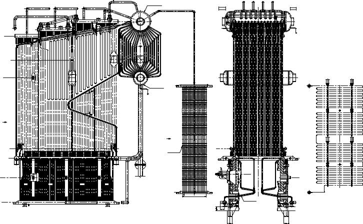
Side |
|
|
|
Top |
. |
|
|
C |
|
|
|
L of |
|
|
|
LRSB |
|
|
|
C |
|
|
|
L of |
|
|
|
man hole & |
|
|
|
peep hole |
|
|
|
A |
|
|
|
C |
EW |
|
|
|
|
|
|
L of over |
|
|
|
fire air at |
|
|
|
L.H.S & R.H.S |
|
|
|
C of |
|
|
|
L |
|
|
|
man hole & |
|
|
|
peep hole |
|
|
|
|
Future |
Future |
Future |
Bed |
|
|
|
wal HDR. |
|
|
|
HD |
|
|
|
evaporato |
|
|
|
(c) |
|
|
|
|
|
|
p |
|
|
|
reader |
Steam drum |
|
|
C of s |
|
|
LHS |
|
|
|
Main steam |
|
|
|
outlet |
|
Water drum |
Eco.outlet |
|
|
HDR. |
|
||
|
E |
|
|
|
|
C |
|
|
|
L of over |
|
|
ECO.coil |
fire air at |
|
|
L.H.S & R.H.S |
||
|
Tube |
||
|
|
|
|
|
|
|
L |
21×70 = 1470 |
Bed evaporator
EW
250
View–A
RHS
Design parameters:
01. |
Design pressure |
: 77.0 kg/cm2(g) |
02. |
Design temperature |
: 320 °C |
03. |
Super heater outlet pressure |
: 67 kg/cm2(g) |
04. |
Super heater outlet temperature |
: 500 °C |
05. |
Total evaporation |
: 25000 kg/hr |
Brief description of boiler:
Natural circulation, Bi–Drum, bottom supported, membrane type, fluidised bed combustion boiler.
C boLof iler
 C of manhole
L
 & peep holes
View–E
50
Engineers Plant and Process For Boilers: Heat Waste and Generators Steam
r Rl

 Steam drum
|
Economiser |
|
|
Burner |
S.S.H |
Chimney |
|
Bank tubes |
|||
|
|||
|
|
||
|
Furnace |
|
|
|
P.S.H |
|
|
|
|
Hot air |
|
|
Air preheater–II |
to windbox |
|
|
Air preheater–I |
Air from |
|
|
FD fan |
||
|
Mud drum |
|
|
|
Hot air from |
|
|
|
air heater |
|
(d)General arrangement of medium pressure and temperature oil & gas fired boiler
FIGURE 2.5 (Continued)
(c) Steam generator for medium-pressure steam. (Courtesy of Thermodyne Technologies, Chennai, India.) (d) Low-pressure steam generator with large evaporator. (Courtesy ISGEC Heavy Engineering Ltd, India.)
Design Furnace Generator Steam
51
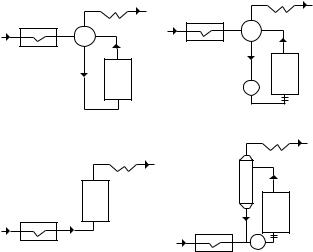
52 |
Steam Generators and Waste Heat Boilers: For Process and Plant Engineers |
The liquid heat or the energy absorbed in the economizer is not much compared to highpressure boilers, and hence, it is small.
Figure 2.5c shows a steam generator for a high-pressure boiler (11,000 kPa). The liquid heat (or the energy absorbed in the economizer) is large, and hence, we see a large economizer. The latent heat is small, and hence, we have only the furnace to absorb the latent heat and a large superheater for the superheat. Since the design pressure is rather high, an external steam drum is used with high ligament efficiency in order to reduce its thickness. Locating the drum up above also helps in improving circulation through the furnace tubes.
Circulation Systems
Furnaces may be classified based on the circulation of steam–water mixture through the evaporator tubes. Natural circulation is common as it requires no external force to aid circulation (Figure 2.6). The density difference between the colder and denser water in the downcomers and the hotter less dense steam–water mixture in the evaporator or furnace tubes aids the circulation process. Natural circulation systems are used up to 165 barg (2400 psig) steam. Beyond this pressure, a circulation pump is used to force the steam– water mixture through the furnace tubes. In once-through boilers, there is no circulation system, and the water entering the boiler comes out as steam. Flow velocity inside the tubes of about 1–1.5 m/s and zero solids in the feed water are desirable to avoid stagnation of flow and deposition of solids inside evaporator tubes causing overheating and possible tube failures. Once-through designs may be used at any steam pressure, but above the critical pressure of steam, only once-through is possible as the liquid–steam phase is absent. Forced circulation designs are described later. Chapter 3 shows a forced circulation steam generator used in oil field application. Here due to the horizontal arrangement of the furnace, circulation pumps are used to force the boiler water from the drum through the furnace tubes back to the drum.
|
|
3 |
|
3 |
|
1 |
|
|
|
|
|
|
|
|
4 |
|
|
|
4 |
|
|
|
|
|
|
|
|
|
|
|
|
|
|
1 |
|
|
|
|
2 |
6 |
2 |
|
|
|
|
||
|
|
|
|
5 |
|
|
|
|
|
|
|
(a) |
|
|
|
(b) |
|
|
|
|
|
3 |
|
|
|
|
3 |
|
|
|
|
|
|
7 |
|
1 |
|
2 |
|
2 |
|
|
|
|
|
||
|
|
|
|
1 |
5 |
|
|
|
|
6 |
|
(c) |
|
|
|
(d) |
|
FIGURE 2.6
Boiler circulation methods. (a) Natural; (b) forced circulation; (c) once-through; and (d) once-through with superimposed circulation. Note: (1) Economizer; (2) furnace; (3) superheater; (4) drum; (5) orifice; (6) circulating pumps.

Steam Generator Furnace Design |
53 |
Furnace Exit Gas Temperature Evaluation
Furnace has been often described as the heart of the boiler. Hence, its sizing assumes paramount importance. Too large a furnace would be expensive. The furnace exit gas temperature will also be low resulting in larger surface area requirements for superheaters and evaporators downstream of the furnace. Too small a furnace can cause overheating of superheater tubes, and if ash-containing oil fuels are fired, slagging or melting of ash can occur causing high-temperature corrosion problems in the superheaters. Hence, the furnace duty or energy absorbed by steam in the furnace, which also fixes the furnace exit gas temperature, should be evaluated with care. Note that the determination of furnace exit gas temperature is not an accurate science and has to be linked with the type of furnace, excess air, flue gas recirculation (FGR) rate used, location of burners, and boiler load. Hence, there is no universally accepted procedure for this calculation.
For the process and plant engineers, a simplified procedure for estimating the furnace performance is given here. Energy balance yields the following equation:
Qf = Ap w fσ(Tg4 − To4) = Wf × LHV × (1 – casing loss-unaccounted loss) − Wg × he (2.1)
where
Qf is the energy transferred to the boiler furnace, kW Wf, Wg is the fuel, flue gas flow, kg/s
LHV is the lower heating value of fuel, kJ/kg
he is the enthalpy of flue gas at furnace exit, kJ/kg
Ap is the effective projected area of the furnace cooling surface, m2w, f is the emissivity of wall and flame
σ is the Steffan–Boltzman constant = 5.67 × 10⁻⁸ W/m2 K4
Tg, To is the furnace gas temperature, and furnace tube wall temperature, K
Tg is defined in a few ways. Some use the furnace exit gas temperature itself for Tg, while some others use the adiabatic combustion temperature. A reasonable agreement between measured and predicted values of the furnace exit gas temperature prevails when Tg is taken as the furnace exit gas temperature plus 160°C–175°C. Using the procedure and example discussed in Appendix A, one may arrive at the furnace exit gas temperature from economizer exit gas temperature. A correlation may be developed based on heat input and the furnace exit gas temperature for a given type of furnace.
The emissivity of wall w varies depending on whether the furnace surfaces are clean or covered with slag. It can vary from 0.6 to 0.9. Soot blowing also changes this value considerably. Flame emissivity f is given by
f = β(1 – e–KPL) |
(2.2) |
where
P is the gas pressure in atmospheres L is the beam length of the furnace, m
K is the attenuation factor that depends on the fuel type and presence of ash and its concentration. For a nonluminous flame,
K |
= (0.8 + 1.6Pw )× (1 − 0.00038Tg )× |
|
(Pc + Pw ) |
(2.3a) |
|
0.5 |
|||
|
|
(Pc + Pw )L |
|
|
54 |
Steam Generators and Waste Heat Boilers: For Process and Plant Engineers |
Pc and Pw are partial pressures of CO2 and H2O in atm. For a semiluminous flame, the ash particle size and concentration enter into the calculations.
K = (0.8 |
+ 1.6Pw )× (1 |
− 0.00038Te )× |
|
(Pc + Pw ) |
|
+ |
7µ |
|
|
(2.3b) |
||
(Pc + Pw )L |
0.5 |
(dm |
Te |
2 |
) |
0.33 |
||||||
|
|
|
|
|
|
|
2 |
|
|
|
|
|
where
dm is the mean effective diameter of ash particles in microns
µm = 13 for coals ground in ball mills, 16 for coals ground in mediumand high-speed mills, and 20 for coals ground in hammer mills
µis the ash concentration in g/Nm3
β= flame filling factor = 1.0 for nonluminous flames, 0.75 for luminous sooty flames of liquid fuels, and 0.65 for luminous and semiluminous flames of solid fuels. For a
luminous oil or gas flame, K = 0.0016Te − 0.5, where Te, the furnace exit gas temperature, is in K.
These equations give only a trend or an approximation for the evaluation of furnace exit gas temperature. A wide variation between measured and estimated furnace exit gas temperature can exist due to the combustion process, location of the burners, type of firing (corner or front wall), how large the furnace is, and how much of it is filled with the flame whether there are soot particles in the fuel to mention a few. The unfilled portions are subject to gas radiation only, and the emissivity (0.15–0.3) can be far less than that estimated for a luminous flame.
In practice, many flames are a combination of luminous and nonluminous portions. The
emissivity then is obtained by combining the two.
f = m l + (1 − m) n where f, l, n are emissivity of flame, luminous, and nonluminous portions and m is a coefficient. For natural gas, m = 0.1, while for fuel oils, it is 0.55. For solid fuels, since the flame is bright all over the furnace, m = 1.
Charts are available to estimate the furnace exit gas temperature directly based on furnace net heat input and its effective projected cooling area as shown later. However, the charts are developed based on furnace type and burner arrangement and evaluation of field data as discussed in Appendix A. Hence, each boiler manufacturer may have his chart or correlations for furnace performance evaluation, and no universal procedure exists as in the case of estimation of convective heat transfer coefficients. Furnace performance evaluation is described by a few as black magic and an art. The following chart shows how the furnace exit gas temperature varies with different fuels, and Figures 2.7 and 2.8 show how the furnace exit gas temperature varies with net heat input for different fuels. Corrections have to be made for various factors such as excess air, FGR, and burner location based on field data and experience.
Example 2.1
Determine the furnace exit gas temperature when natural gas (methane = 97%, ethane 3% by volume) is fired in a boiler furnace at 15% excess air. The net heat release rate per effective area is 250 kW/m2. Furnace dimensions are approximately 2.44 m wide, 3.35 m high, and 9.75 m long (EPRS = 127 m2). Flue gas analysis % volume CO2 = 8, H2O = 18, N2 = 71.5, O2 = 2.5. The tube walls may be assumed to be at 660 K. Its method of estimation is discussed later.

Steam Generator Furnace Design |
55 |
Furnace exit temperature, °C
1400 |
|
|
|
|
|
|
|
|
1 |
|
|
|
|
|
|
|
|||
|
|
|
|
|
|
|
|
|
|
1300 |
|
|
|
|
|
|
|
|
2 |
|
|
|
|
|
|
|
|
|
3 |
1200 |
|
|
|
|
|
|
|
|
4 |
1100 |
|
|
|
|
|
|
|
|
5 |
|
|
|
|
|
|
|
|
|
|
1000 |
|
|
|
|
|
|
|
|
|
900 |
|
|
|
|
|
|
|
|
|
800 |
|
|
|
|
|
|
|
|
|
120 |
170 |
220 |
270 |
320 |
370 |
420 |
470 |
||
Net heat input, kcal/m2 h
FIGURE 2.7
Typical furnace exit gas temperatures for some fuels: (1) pulverized coal, (2) natural gas, (3) fuel oils, (4) grate fired bagasse, (5) grate fired coal. (1 is the topmost curve and 5 is the bottommost curve.)
FOT, °C
1400
1350
1300
1250
1150
1100
1050
1000
150 |
200 |
250 |
300 |
350 |
400 |
450 |
500 |
550 |
600 |
1200 |
|
|
|
|
|
|
|
|
Gas |
|
|
|
|
|
|
|
|
|
Oil |
Net heat release rate, kW/m2
FIGURE 2.8
Furnace exit gas temperature for oil and natural gas. (From Ganapathy, V., Industrial Boilers and HRSGs, CRC Press, Boca Raton, FL, 2001, p112.)
The calculation of net heat release rate itself involves the following steps:
•Calculation of boiler duty (energy absorbed by steam) in kW.
•Calculation of boiler efficiency (see Chapter 1), from which the fuel flow is obtained.
•Net heat input (fuel flow × LHV).
•Net heat input divided by furnace effective projected radiant surface area (water-cooled surfaces). (For surfaces covered with refractory, a multiplication factor of 0.1–0.2 is used.)
Assume one has done all the calculations given earlier. From combustion calculations (Chapter 1), it can be shown that the HHV of the fuel gas = 55,345 kJ/kg and its LHV = 49,915 kJ/kg.
It may be shown that each GJ of natural gas fired on HHV basis requires a theoretical amount of 314 kg of dry air (Table 1.2). This amount of heat input requires
56 |
Steam Generators and Waste Heat Boilers: For Process and Plant Engineers |
1 × 10⁶/55,345 = 18.07 kg of fuel. So ratio of dry air to fuel is 314/18.07 = 17.37, or at 15% excess air, dry air per kg fuel is 1.15 × 17.37 = 19.97 or wet air about 20 kg/kg fuel as air always contains some moisture. Hence, the ratio of flue gas to fuel is 19.97 + 1 = 20.97. If wet air is considered, the ratio of flue gas to fuel Wg/Wf is about 21. From energy balance in the furnace, we can write the following:
From (2.1), Qf = Ap w fσ(Tg4 − To4) = Wf LHV – Wg he (heat losses are on the order of 0.5% in oiland gas-fired boilers and hence neglected). Dividing by Wf, we have
Ap w fσ (Tg4 − To4)/Wf = LHV − Wg he/Wf or
Qf/Ap = 250,000 W/m2 = Wf × LHV/Ap. Rearranging the terms, Ap/Wf = LHV/250,000 = 49,915,029/250,000 = 199.7 m2 s/kg
Pc = 0.08, Pw = 0.18. Assume furnace exit gas temperature Te = 1150°C. hg = 1430.49 kJ/kg (see Appendix F). Use Tg = 1150 + 170 = 1320°C = 1593 K (170°C more than the FEGT [furnace exit gas temperature])
K = (0.8 + 1.6Pw )× (1 − 0.00038Te)× |
(Pc + Pw ) |
|
|||||
|
0.5 |
|
|
||||
|
|
|
(Pc |
+ Pw )L |
|
||
1.7 |
|
|
|
|
|
|
|
L = |
|
= |
2.09 m |
|
|||
(1/2.44 + 1/3.35 + 1/9.75) |
|
||||||
K = (.8 + 1.6 × .18)× (1 − .00038 × 1423)× |
|
(0.26) |
|
= 0.176 |
|||
(0.26 × 2.09)0.5 |
|||||||
f = (1 − e−.176 × 2.09) = 0.308. Let emissivity of walls w = 0.9
From (2.3),
LHS (left-hand side) = 199.7 × 0.9 × .308 × 5.67 × 10–8 × (15934 – 6604) = 19.61 × 10⁶ W
RHS = 49,915,029−21 × 1,430,490 = 19.93 × 10⁶ W
Hence, furnace exit gas temperature is close to 1150°C.
It may be noted that furnace duty estimation is an iterative process. We have assumed an efficiency to obtain the fuel input. In reality, one has to assume the furnace size, obtain the furnace duty, and then design the heating surfaces downstream of the furnace to obtain the desired exit gas temperature that matches the efficiency used or use the efficiency obtained in the earlier calculations. A well-written computer program is the solution. The earlier example is to explain the methodology only.
The furnace net heat input = 250 × 127 = 31,750 kW. Fuel input = 31,750/49,915 = 0.636 kg/s. Flue gas generated = 0.0636 × 21 = 13.357 kg/s
The furnace duty = 31,750−13.357 × 1430.49 = 12,642 kW. The average heat flux = 12,642/127 = 99.5 kW/m2
Example 2.2
In the same furnace if no. 2 oil at 15% excess air is fired, then determine the exit gas temperature. Flue gas analysis is CO2 = 12, H2O = 12, N2 = 73.5, O2 = 2.5. Fuel oil LHV = 43,050 kJ/kg and HHV = 45,770 kJ/kg. Net heat input is the same as before, namely, 250 kW/m2.
Solution
Ap/Wf = LHV/250,000 = 43,050 × 103/250,000 = 172.2 m2 s/kg
Assume furnace exit gas temperature is 1050°C = 1323 K.
K = (0.8 + 1.6 × 0.12)× (1 − 0.00038 × 1323)× 0.24/(0.24 × 2.09)0.5 = 0.167
Steam Generator Furnace Design |
57 |
For theoretical combustion of fuel oil, 1 GJ heat put requires 320 kg of dry air (see Chapter 1). Or 1 × 10⁶/45,770 = 21.85 kg of fuel requires 320 kg dry air. Or ratio of flue gas to fuel at 15% excess air = 1.15 × 320/21.85 + 1 = 17.84 or say 18 kg/kg wet air.
For a luminous flame, the emissivity consists partly of luminous and a nonluminous portion. Then f = 0.55 × l + .45 × nl
K = .0016 × 1323 − .5 = 1.616. l = 0.75 × (1 − e−1.616×2.09 ) = 0.724
nl = (0.8 + 1.6 × .12)× (1 − .00038 × 1323)× .24 /(.24 × 2.09)0.5 = 0.167. Hence, f = 0.55 × 0.724 + .45 × 0.167 = 0.473
LHS = 172.2 × 0.473 × 0.9 × 5.67 × (14.934 − 6.64) = 19.86 × 10⁶ W (Here again, we added 170°C to the assume FEGT.)
RHS = 43.05 × 10⁶−18 × 1,296,280 = 19.72 × 10⁶ W
Hence, furnace exit gas temperature is close to 1050°C.
This is only an estimate. It is preferable to use charts developed based on field data and experience as shown in Figure 2.8. Furnace exit gas temperature is a function of so many variables as mentioned earlier. Hence, experience and field testing can provide more reliable data for a particular furnace configuration. One may also work backward from economizer exit and use the field data to establish Te as discussed in Appendix A.
Once the furnace exit gas temperature is estimated, the furnace duty has to be computed. This is discussed later.
Empirical Formula for Furnace Duty Estimation
In European and Russian boiler calculation practice, the Gurvich method has found wide acceptance. The following equation relates the furnace exit gas temperature Te with combustion temperature Tc [2].
Te |
= |
B0.6o |
(2.4) |
Tc |
(Bo0.6 + Maf0.6 ) |
where
Te, Tc are the furnace exit gas temperature and adiabatic combustion temperatures M is an empirical factor impacted by fuel and gas temperature profile in the furnace Bo is the Boltzman number
Bo = |
ϕWfVc |
(2.5) |
(σψApTe ) |
where
Vc is the average heat capacity of the flue gas in the furnace in the range of (Tc – Te) formed by 1 kg of fuel burned, kJ/kg K
φ is the furnace efficiency or (1-% heat loss/100) and is typically 0.995 σ is the Stefan–Boltzman constant = 5.67 × 10⁻¹¹ kW/(m2 K4)
ψ is an empirical factor = xζ
ζ is 0.55 for fuel oil and 0.65 for gas

58 |
Steam Generators and Waste Heat Boilers: For Process and Plant Engineers |
For coal firing, it varies from 0.35 to 0.55. For refractory-covered surfaces, it is 0.1–0.2. ζ is corrected by a factor y dependent on the furnace wall tube spacing to diameter. For pitch to diameter ST/d of 1.25, it is 0.97, and for ST/d of 2, it is 0.82. If the furnace has different sections with different tube spacing or partly covered with refractory, one may use the following weighted average value of ψ.
ψ = ∑yi Api ζi/Ap |
(2.6) |
af = coefficient of thermal radiation = 1/[1 + {1/ f − 1}ψ] |
(2.7) |
Flame emissivity f has been discussed earlier for nonluminous and luminous flames.
M = a coefficient = A − BX |
(2.8) |
where A and B are empirical coefficients depending on fuel fired. For gas and oil, A = 0.54 and B = 0.2. For coal, A = 0.59 and B = 0.5. X is the relative position of the highest temperature zone in the furnace (Figure 2.9a). If x1 is the distance of burner 1 from bottom of
Burner 1 |
x1 |
|
Burner 2 |
||
x2 |
||
|
(a)
Temperature (°F)
3250
2975
2700
2425
2150
1875
1600
1325
1050
775
500
y
x z
(b)
FIGURE 2.9
(a) Temperature profiles along furnace length or height (x1, x2 measured from furnace bottom). (b) CFD modeling of furnace temperature profile.
Steam Generator Furnace Design |
59 |
furnace and x is the distance from bottom of furnace to furnace exit, then X is the relative position = x1/x. If the burner is in the front wall as in a D-type boiler, one may use X = 0 as x1 is 0. Chapter 1 shows how one may estimate the adiabatic combustion temperature Tc for various fuels from excess air.
Te = |
1 |
|
(2.9) |
|
[M{5.67 10−11ψApafTc3/(ϕWf Vc )}0.6 |
+ 1] |
|||
Tc |
|
Tc is obtained through combustion calculations as shown in Chapter 1. It is a function of excess air, combustion air temperature, and fuel analysis. Wf = fuel input kg/s.
Example 2.3
Solve Example 2.1 using Gurvich method. The boiler generates 45,372 kg/h (100,000 lb/h) steam at 25 kg/cm2 g (355 psig) using 105°C (221°F) feed water. Natural gas at 15% excess air is fired as in Example 2.1. Compute also the energy absorbed in the furnace. D-type boiler with burner at front walls is used. The furnace is completely water cooled. No refractory is used. Pitch-to-diameter ratio of tubes is 1.75. LHV = 49,884 kJ/kg. Ambient air enters the furnace, and hence, additional heat input by air is not considered.
Solution
Data such as flue gas and combustion temperature and ratio of flue gas to fuel are obtained from combustion calculations (Chapter 1). Assume boiler heat losses = .5%. Hence, φ = 0.995. Furnace projected area based on using 253 kW/m2 net heat input is 127 m2. Adiabatic combustion temperature = 1780°C = 2053 K. Fuel quantity = 2344 kg/h = 0.651 kg/s.
Flue gas quantity = 49,216 kg/h = 13.67 kg/s. Ratio of flue gas to fuel = 49,216/234 = 21. ψ = 0.88 × 0.65 = 0.572. f = .308 from Example 2.1. af = 1/[1 + {1/0.308 − 1}]0.572] = 0.437. Assume Te = 1150°C. From the properties of flue gases, enthalpy of gases (from Appendix F) at 1780°C and 1150°C = 565 kcal/kg and 342 kcal/kg. Hence, Vc = 21 ×
(565 – 342)/(1780 – 1150) = 7.43 kcal/kg K = 31.1 kJ/kg K. M = 0.54 as the burners are on front wall.
Hence, Te/Tc = 1/[M{5.67 × 10–11 ψAp af Tc3/(φWf Vc)}0.6 + 1] = 1/[0.54{5.67 × 10–11 × 0.572 × 127 × 0.437 × 20533/(0.995 × 0.651 × 31.1)}0.6 + 1] = 0.683 or Te = 2053 × 0.683 = 1402 K = 1129°C. Enthalpy of flue gas at 1129°C from Appendix F is 335.5 kcal/kg = 1404.7 kJ/kg.
Hence, furnace duty Qf = 0.651 × 49,915−21 × .651 × 1404.7 = 13,291 kW (45.36 MM Btu/h). The average heat flux is then Qf/Ap = 13,291/127 = 104.6 kW/m2 (33,055 Btu/ft2 h). To estimate the fin tip temperature or CHF-related issues, the maximum heat flux consid-
ering the variation in temperature profile of the flue gas is considered.
One has to increase the furnace area in case the furnace exit gas temperature is high and is likely to cause slagging problems at the furnace exit. However, the example is shown to illustrate the methodology.
Example 2.4
Estimate the furnace exit gas temperature using the Gurvich method when fuel oil is fired in the same furnace. LHV of fuel oil = 43,059 kJ/kg. Fuel quantity = 0.755 kg/s. Use the data from Chapter 1. Fifteen percent excess air is used. Air enters at ambient temperature.
Adiabatic combustion temperature = 1866°C = 2139 K and ratio of flue gas to fuel = 17.83 from Chapter 1. Fuel quantity = 2718 kg/h = 0.755 kg/s.
ψ = 0.88 × 0.55 = 0.484. f = 0.473 from Example 2.2. af = 1/[1 + {1/0.473 − 1}]0.484] = 0.65

60 |
Steam Generators and Waste Heat Boilers: For Process and Plant Engineers |
Assume Te = 1100°C. From the properties of flue gases, enthalpy of gases (from Appendix F) at 1866°C and 1100°C = 572 kcal/kg and 314.7 kcal/kg. Hence, Vc = 17.83 × (572 – 314.7)/(1866 − 1100) = 5.99 Kcal/kg K = 25.07 kJ/kg K. M = 0.54 as the burners are on front wall.
Hence, Te/Tc = 1/[M{5.67 × 10–11ψAp af Tc3/(φWf Vc)}0.6 + 1] = 1/[0.54{5.67 × 10–11 × 0.484 × 127 × 0.65 × 21393/(0.995 × 0.755 × 25.07)}0.6 + 1] = 0.6267 or Te = 2139 × 0.6267 = 1341 K = 1068°C. Enthalpy of gas at 1068°C is 304.4 kcal/kg = 1274.5 kJ/kg.
Furnace duty Qf = 0.755 × 43,059–17.83 × 0.755 × 1274.5 = 15,352 kW (52.4 MM Btu/h). The heat flux and furnace duty are higher on oil firing. Hence, the circulation is checked based on heat flux obtained in oil-fired case. The furnace exit gas temperature is also lower on oil firing compared to natural gas. When a boiler is fired with both fuel oil and natural gas, it is common practice to design the boiler and superheater surfaces on oil firing to ensure the desired steam temperature is obtained and, when firing natural gas, the superheater steam temperature will only be higher, which can be controlled
by various methods as discussed in Chapter 3.
(Note that the terms furnace heat input and furnace duty are different. The duty is used to compute the heat flux inside the tubes and to check for departure from nucleate boiling [DNB]. This is explained later).
It may be noted that the furnace calculations give an idea of the exit gas temperature, and accuracy can vary depending on burner type and location. Boiler designers obtain field data on the performance and work backward the furnace exit gas temperature and arrive at correcting curves. Unlike convective heat exchanger calculations where the correlations for heat transfer are well established and more reliable, furnace performance evaluation is still a gray area. The error in estimation of the furnace exit gas temperature could be as high as ±100°C (180°F).
Furnace Duty with Combination Firing
Example 1.14 showed how the boiler efficiency and other pertinent data may be obtained when multiple fuels are fired in a boiler using field data. To compute boiler efficiency from field data, input the steam parameters, exit gas temperature and % oxygen values (dry or wet), fuel analysis and vary the ratio among fuels fired till the field measured oxygen of 3.46% dry is obtained. It may be possible to measure one of the fuels consumed accurately, and hence, we may cross-check the field data using this information.
The plant engineer may arrive at the furnace exit gas temperature by working backward from the economizer as shown in Chapter 3. The computation of furnace exit gas temperature may be done as follows:
1.Obtain the fuel input on LHV basis for natural gas and oil.
2.Based on the total net heat input of both fuels and the furnace projected area, obtain the furnace exit gas temperature for natural gas and oil. Since the ratio is about 70:30, the furnace exit gas temperature may be approximated as 70% of the value for natural gas and 30% of the value for oil.
3.Then the furnace duty may be estimated by the methods discussed earlier. The mixture flue gas analysis and enthalpy data are used. One may check if the furnace exit gas temperature matches with the value obtained by back calculation and if the total steam duty matches with the sum of the duties of all components. Any difference may be attributed to the estimation of furnace exit gas temperature as it has the largest uncertainty in the estimation process, more so with multiple-fuel firing.

Steam Generator Furnace Design |
61 |
Distribution of Heat Flux around Tubes and Fins
Furnace wall is typically of membrane wall design (Figure 2.10). The tubes are of outer diameter d with tube spacing of ST. Furnace calculations and estimation of duty give some idea of the heat flux in the furnace based on projected area. However, this is an average value, and based on burner location, flame shape, excess air used, and field data on similar units, the boiler designer has some idea of the maximum heat flux. The ratio of maximum to average heat flux may vary from 1.2 to 1.5. Once the maximum flux is determined, one has to see how it varies around the tube periphery and along the fins. The actual flux at a location has to be obtained by multiplying the maximum flux by the view factor. Figure 2.10a shows how the view factor is estimated at any point on the tube and also along the membrane wall. Let us find out the view factor at a point on the tube defined by angle θ (Table 2.1).
Draw a tangent at the point on the circumference at angle θ to the adjacent tube as shown in Figure 2.10a. Draw a tangent at the point on the circumference on the tube itself. Now the angle φ between the two tangents is calculated.
Then view factor corresponding to angle θ is (1 + cos φ)/2.
Similarly, at any point on the fin, as shown in Figure 2.10a, draw two tangents to the adjacent tubes. If φ1 and φ2 are the angles, then
View factor on fin = (cos φ1 + cos φ2)/2
It is clearly seen that at the top of the tube facing the furnace radiation, the angle θ = 90. ϕ = 0. Hence, view factor = 1. At the angle θ = 0, if the fin spacing is 101 mm and tube OD = 50 mm, then the angle θ = 90 + sin−1(25.4/76.2) = 109°. Then cos109° = −0.326 and view factor = (1 − 0.326)/2 = 0.337 as shown in the earlier table.
At the fin midpoint, sin φ1 = sin φ2 = 25.4/50.8 = 0.5. cos 30° = 0.866. Hence, view factor = 0.866. Using the view factors, one may estimate the local heat flux.
Distribution of Radiation to Tube Banks
When boiler screen section or superheater is located at the furnace exit, direct radiation from the furnace is absorbed by these heating surfaces and increases the heat flux inside the tubes and hence the tube wall temperature. This radiation is generally absorbed completely within the first four to five rows of tubes depending on the tube spacing. Figure 2.11 shows the distribution of external radiation to different rows depending on tube spacing. Direct radiation adds to the energy absorbed by the tubes and increases the metal temperature and may cause overheating and thermal expansion problems. Hence, one should be careful while locating superheaters at the furnace exit. When a screen section is used at the furnace exit, the tubes will not be overheated as these tubes operate at slightly above saturation temperature of steam, while a superheater operates at much higher temperature.
The following formula predicts the radiation to the tubes:
|
|
d |
|
d |
|
−1 |
|
d |
|
ST |
2 0.5 |
|
ST |
|
|
|||
|
|
sin |
|
|
|
|
|
|||||||||||
a = 3.14 |
|
|
|
− |
|
|
|
|
|
+ |
|
|
− 1 |
− |
|
(2.10) |
||
|
|
|
|
d |
d |
|||||||||||||
|
|
2ST |
|
ST |
|
|
ST |
|
|
|
|
|
|
|||||
|
|
|
|
|
|
|
|
|
|
|
|
|
|
|
|
|
|
|
where a = fraction of energy absorbed by row 1. The second row absorbs (1 − a)a, the third row, [1 − {a + (1 − a)a}a], and so on.

62 |
Steam Generators and Waste Heat Boilers: For Process and Plant Engineers |
|||||||||||||||||
|
|
|
|
|
|
|
|
qt |
|
|
|
|
||||||
|
|
|
|
|
1 |
|
|
|
|
|
|
|
|
|
|
|
|
|
|
|
|
|
|
|
|
|
|
|
|
|
|
|
|
|
|
|
|
|
|
|
|
|
|
|||||||||||||
|
2 |
|
|
|
|
|
|
|
|
|
|
|||||||
|
|
|
|
|
|
|
|
|
|
|
||||||||
|
|
3 |
|
|
|
|
|
|
|
|
|
|||||||
|
|
|
|
|
|
|
|
|
h |
|
|
|
|
|
||||
|
|
|
|
|
|
|
|
|
st |
|
|
|
|
|||||
|
|
|
|
|
|
|
|
|
||||||||||
|
|
|
|
|
Tube diameter is d |
|
|
|
|
|||||||||
|
|
|
|
|
|
|
|
|
|
|
|
|
N |
|
|
|
|
|
|
|
T |
|
|
|
|
||||||||||||
|
|
|
|
|
|
|
ψ |
|
|
|
B |
|||||||
|
|
|
|
|
|
Φ |
|
|
d/2 |
|||||||||
|
|
|
θ |
|
|
|
|
|||||||||||
|
|
|
|
|
|
|
B = 2h |
|
|
|
|
|||||||
|
T1 |
|
|
|
T2 |
|||||||||||||
|
|
|
|
2 |
|
1 |
|
|
|||
|
|
|
|
|
|
||||||
|
|
|
|
|
|
||||||
|
|
|
|
|
d/2 |
B |
|||||
|
(a) |
|
|
|
|
|
|
|
|
||
|
|
|
|
|
|
|
|
|
|||
|
1.2 |
|
|
|
|
|
|
|
|
|
|
|
|
|
1 |
|
|
|
|
|
2 in. on 4 in. centers |
|
|
|
|
|
|
|
|
|
|
||||
|
|
|
|
|
|
|
3 in. on 3.75 in. centers |
|
|||
|
1 |
|
|
|
|
|
|
||||
|
|
|
|
|
|
|
|
|
|
|
|
|
|
|
|
|
|
|
3 |
||||
|
|
|
|
|
|
|
|
||||
factor |
0.8 |
|
|
|
|
|
|
|
|
|
|
|
|
|
|
|
|
|
|
|
|
||
0.6 |
|
|
|
|
|
|
|
|
|
|
|
View |
|
|
|
|
|
|
|
|
|
|
|
0.4 |
|
|
|
|
|
|
|
|
|
|
|
|
|
|
|
|
|
|
|
|
|
|
|
|
|
|
|
|
|
|
|
|
|
|
|
|
0.2 |
|
|
|
|
|
|
|
|
|
|
|
|
|
|
|
|
|
2 |
|
|
||
|
|
|
|
|
|
|
|
|
|
||
|
0 |
|
|
|
|
|
|
|
|
|
|
|
|
|
|
|
Angle from vertical |
||||||
(b) |
|
|
|||||||||
FIGURE 2.10
(a) View factor estimation. (b) View factors for 2 in OD tube on 4 in and 3 in OD tube on 3.75 in. spacing around tube periphery.

Steam Generator Furnace Design |
63 |
(Fin tip—sat temp.)
h = 0.25, 0.5, 1.0 in.
1.0 in.
0.5
0.25
Heat ux inside tubes
2h
h = Membrane height
(c) |
Heat ux |
|
FIGURE 2.10 (Continued)
(c) Relating fin tip temperature to heat flux.
TABLE 2.1
View Factors for Typical Configurations of Membranes
Angle from Horizontal θ |
View Factor—Case 1 |
View Factor—Case 2 |
|
|
|
0 |
0.33 |
0.17 |
15 |
0.51 |
0.37 |
30 |
0.68 |
0.60 |
45 |
0.82 |
0.79 |
60 |
0.92 |
0.92 |
75 |
0.98 |
0.98 |
90 |
1.00 |
1.00 |
Quarter point on fin |
0.83 |
0.57 |
Midpoint of fin |
0.86 |
0.60 |
Note: Case 1:2 in. OD tubes on 4 in. spacing. Case 2:3 in. OD tube on 3.75 in. spacing.
Example 2.5
A superheater with 50 mm OD tubes at 200 mm spacing is exposed to direct furnace radiation. Estimate the energy absorbed by the first four rows. Assume Qr the direct radiation is 1 MW. (The radiation to the superheater may be estimated based on the heat flux and opening area of the exit plane as discussed earlier.)
Solution
d = 50 mm, ST = 200 mm.
a = 3.14 × 50/2/200 −50/200[sin−1(50/200) + {(200/50)2 − 1}0.5 − 200/50] = 0.3925 − 0.25(0.2526 + 150.5 – 4) = 0.361. Hence, first row absorbs 0.361 MW. (See Figure 2.11, which gives the total energy absorbed from external radiation for a certain number of rows. For two rows, the total absorbed is 0.6 MW as seen from the figure.)
The second row absorbs (1 − 0.361) × 0.361 = 0.2306 MW (total of two rows absorb nearly 0.6 MW). The third row receives [1 − (0.361 + 0.2306)] × 0.361 = 0.147 MW.
The fourth row = [1 − (0.361 + .2306 + 0.147)] × 0.361 = 0.094 MW and so on. Typically, a minimum of four rows will absorb the external radiation completely. If
the tube spacing were smaller, then a large amount of radiation is absorbed within the first few rows resulting in high heat flux to these tubes; hence, it is better to use a wider

64 |
Steam Generators and Waste Heat Boilers: For Process and Plant Engineers |
|
1.0 |
|
|
|
|
|
|
|
|
|
|
|
|
|
|
0.9 |
|
|
|
|
|
|
|
|
24 |
|
|
|
|
|
|
|
|
|
|
|
|
|
|
22 |
|
|
|
|
|
0.8 |
|
|
|
|
|
|
|
|
20 |
|
|
|
|
|
|
|
|
|
|
|
|
|
18 |
|
|
|
|
|
|
|
|
|
|
|
|
|
|
|
16 |
|
|
|
|
|
0.7 |
|
|
|
|
|
|
|
|
14 |
|
|
|
|
|
|
|
|
|
|
|
|
|
12 |
|
|
|
|
|
|
|
|
|
|
|
|
|
|
|
|
|
|
|
|
|
0.6 |
|
|
|
|
|
|
|
|
10 |
|
|
|
|
Kn |
|
|
|
|
|
|
|
|
|
9 |
|
|
|
|
0.5 |
|
|
|
|
|
|
|
|
8 |
|
|
|
|
|
|
|
|
|
|
|
|
|
7 |
|
|
|
|
||
|
|
|
|
|
|
|
|
|
|
|
|
|
|
|
|
0.4 |
|
|
|
|
|
|
|
|
6 |
|
|
|
|
|
|
|
|
|
|
|
|
|
5 |
|
|
|
|
|
|
|
|
|
|
|
|
|
|
|
|
|
|
|
|
|
0.3 |
|
|
|
|
|
|
|
|
4 |
|
|
|
|
|
|
|
|
|
|
|
|
|
3 |
|
|
|
|
|
|
|
|
|
|
|
|
|
|
|
|
|
|
|
|
|
0.2 |
O STO |
|
|
|
|
|
|
2 |
No. of rows deep n |
|
|||
|
0.1 |
O |
O |
|
|
|
|
|
|
1 |
|
|
|
|
|
O |
O |
|
|
|
|
|
|
|
|
|
|
||
|
0 |
Gas ow |
|
|
|
|
|
|
|
|
|
|
|
|
|
2 |
4 |
6 |
8 |
10 |
12 |
14 |
16 |
18 |
20 |
22 |
24 |
26 |
|
|
1 |
|||||||||||||
|
|
|
|
|
|
|
|
ST/d |
|
|
|
|
|
|
FIGURE 2.11
Distribution of external radiation to tubes.
spacing when the external radiation is large so that the radiation is spread over more rows, and heat flux is not intense in the first two or three rows. Screen tubes in boilers and heaters perform this function. Good boiler designs shield the superheater from furnace radiation by using more than six to eight rows of screen tubes. This is discussed in Chapter 3 on steam generators.
Relating Heat Flux from Furnace to Inside Tubes
The average or maximum heat flux in the furnace may be estimated using the methods suggested earlier. However, in order to check for DNB and also to estimate the boiling heat transfer coefficients, the heat flux inside the tubes is required.
From Figure 2.10,
qpST = qc(πd/2 + 2h) |
(2.11) |
where qc is the average heat flux referred to the developed surface or periphery. Then,
qc d/di = qi
where
d, di refer to tube OD and ID, mm h is the membrane height, mm ST is the tube spacing, mm
qp is the heat flux on projected area basis, kW/m2 qc is the circumferential heat flux, kW/m2
qi is the heat flux inside the tubes, kW/m2

Steam Generator Furnace Design |
65 |
Simplifying,
qi = qp STd/{(πd/2 + 2h)di}
Example 2.6
If qp = 87.5 kW/m2, d = 51 mm, di = 44 mm, h = 15 mm, ST = 81 mm, then
qi = 87.5 × 81 × 51/(3.14 × 51/2 + 30)/44 = 74.6 kW/m2
One may correct for the heat flux distribution along the flame length (see Figure 2.9 for vertical and horizontal furnaces) and use these values to check for DNB as discussed later.
External Radiation to Heat Transfer Surfaces at Furnace Exit
The calculations provided earlier give an estimate of energy absorbed by the furnace. However, there will be direct radiation to heat transfer surfaces such as superheaters or boiler screen section at furnace exit. One may estimate this as follows:
The energy absorbed by furnace from Example 1 = 12,642 kW. The furnace area = 127 m2. The average heat flux = 99.5 kW/m2. Let the opening at furnace exit = 3.35 × 1.2 = 4 m2. Then approximately 99.5 × 4 = 398 kW energy is radiated to the tube section at furnace exit. However, one has to correct for the actual emissivity at the furnace exit and the smaller beam length and the distribution of heat flux along the flame length. Equations and charts are available in Ref. [7] for estimating the correction factor, and it may be seen that about 0.5–0.6 times the average flux is radiated to the surfaces beyond the furnace. Hence, the direct radiation may be taken as 250 kW, and the furnace absorbs 12,642 − 250 = 12,392 kW. If the screen section is located at the furnace exit, then this radiant energy is added to the evaporator duty; thus the external radiation does not cause any concern when the screen section absorbs this radiation as the boiling coefficient inside tubes is high and does not increase the tube wall temperature much; however, when a superheater is located at the furnace exit, then this has to be considered as contributing to the superheater duty. The first few rows of tubes depending on tube spacing will receive this external radiation and can overheat the superheater tubes. The distribution of external radiation to tube bank was discussed earlier. The first four to five rows typically absorb this radiation completely with the first row bearing the maximum brunt.
If we estimate the gas emissivity at the furnace exit and compute the external radiation, we get a different value for external radiation. From Example 2.1, Pc = 0.08, Pw = 0.18. At the furnace exit and opening to the convection bank, the beam length is different. Using a width of 2.44 m, height = 3.35 m, and length = 1.2 m,
L = 1.7/(1/2.44 + 1/3.35 + 1/1.2) = 1.1 m.
K = (.8 + 1.6 ×.18) × (1 − 0.00038 × 1423) × (0.26)/(0.26 × 1.1)0.5 = 0.24
f = (1 − e−.24 × 1.1) = 0.23. Let w = 0.9
66 |
Steam Generators and Waste Heat Boilers: For Process and Plant Engineers |
Direct radiation to furnace opening to tubes at, say, 660 K = 5.67 × 10–11 × 0.23 × 0.9 × (14234 − 6604) × 4 = 184 kW. (Opening to furnace = 3.35 × 1.2 = 4 m2)
Let us say that we have located the radiant superheater at the furnace exit (not a good idea). Let there be 12 tubes of diameter 50.8 and length 3.35 m facing the furnace at a spacing of 100 mm. One can estimate the average heat flux in the furnace and the energy radiated at the furnace exit as discussed earlier and compute the energy absorbed row by row. The fraction a absorbed by the first row is given by
a = 3.14 (d/2S) − d/S[sin−1(d/S) + {(S/d)2 − 1}0.5 − S/d]
For a ST/d = 2, a = 3.14/4 – 0.5 × [sin−1(0.5) + 300.5 − 2] = .785 − 0.5 × [0.523 + 1.732 − 2] = 0.66 [the value for sin-1(0.5) is in radians].
The first row absorbs the maximum of 66% of the external radiation. Let 0.66 × 184 = 121 kW of energy be absorbed in the first row. Then the additional heat flux due to direct radiation is 121 × 860 = 104,438 kcal/h. If the steam generation is 40,000 kg/h, and there are 20 streams in 5 tubes/row (on each header) and 4 along gas path with 3 passes in 12 rows (see Figure B.4h for explanation of streams), flow through each tube will be about 2,000 kg/h. With a baffle after every 4 rows of tubes, the additional enthalpy absorbed by steam is (104,438/12/2,000) × 3 = 13 kcal/kg. Assuming steam-specific heat of 0.65 kcal/kg °C, the additional pickup in steam temperature and wall temperature can be at least 20°C. This can decrease the life of the superheater by several years if you check using the LMP charts for the material in consideration (see Appendix E). The tubes may be even operating well above their limits and can fail. Hence, locating the superheater at the furnace exit is not good practice as discussed in Chapter 3. Advantages of convective superheater design have been elaborated in Chapter 3. Due to mixing with slightly cooler steam in subsequent rows away from the furnace, the enthalpy total pickup by the first row could be slightly less but still a factor to be considered. If, for argument, we assume the first row facing the furnace starts out at 350°C and gets heated to 400°C, then this row can pick up an additional 20°C as shown and can cause overheating. Several superheaters located at furnace exit have failed for this reason. Also we estimate a particular furnace exit gas temperature. What if it is about 50°C higher? The radiation will be about (1473/1423)4 or 15% more, or the temperature increase is higher by 23°C.
Direct Radiation to Superheater at Part Load
Let us see what happens to the direct radiation at part loads. Taking proportionate values, at 60% load, the NHI/EPRS value may be taken as 0.6 × 250 = 150 kW/m2. The furnace exit gas temperature is about 1050°C from Figure 2.8. The external radiation to the first row is = 0.66 × 5.67 × 10–11 × 0.23 × 0.9 × (13234 − 6604) × 4. = 99 kW = 85,140 kcal/h. The steam flow is 24,000 kg/h. The additional enthalpy absorbed by row 1 facing the furnace will be (85,140/12/1,200) × 3 = 18 kcal/kg or a temperature rise of 27°C (compared to 20°C at 100% load). This characteristic of radiant superheaters is shown in Figure 3.28.
That is why plant engineers should be concerned about purchasing boilers with a radiant superheater. Operating it at low loads is also a risk as discussed in Chapter 3. Unless a good screen section is used with a minimum of four to five rows, the external radiation can play havoc with the tube temperature and the life of the superheater. The other issues with radiant superheater design are discussed in Chapter 3.
Steam Generator Furnace Design |
67 |
Terms Frequently Used in Furnace Performance
Area heat release rate: This is the heat input on HHV basis divided by the furnace effective projected radiant surface area or also called EPRS, m2. If air-heating is absent, AHRR will be fuel fired (kg/s) × HHV(J/kg)/EPRS(m2). The units are in kW/m2 (Btu/ft2 h)(kcal/m2 h).
EPRS: Effective projected radiant surface is the total projected area of the furnace walls, which are effective (water-cooled membrane walls) less the openings for burners and manways. If refractory is used on some surfaces, the effectiveness is reduced by using appropriate multiplication factor of 0.1–0.2 discussed elsewhere. The opening to the convection pass is also included in this estimation of EPRS.
Volumetric heat release rate: This is fuel input on HHV basis divided by the volume of furnace (kW/m3)(Btu/ft3h)(kcal/m3h).
Furnace duty: Energy absorbed by furnace, kW (MM kcal/h)(MM Btu/h).
Net heat input: This is the heat input to the furnace based on LHV of the fuel; unaccounted and casing loss are considered in its estimation and also heat input from air if any.
Heat flux: This is the energy converted to tube side divided by inner surface area of the tubes in the furnace (kW/m2) (kcal/m2 h) (Btu/ft2 h). Table 2.2 gives an idea of the various terms and the units.
Estimating Boiling Heat Transfer Coefficient
An idea of boiling heat transfer coefficient helps in evaluating the tube wall temperature and the membrane tip temperature. Tube wall temperature is also required to estimate the interchange of radiation energy between the hot flue gas and the membrane walls. Subcooled boiling heat transfer coefficient inside tubes for water may be estimated by the following equations:
According to Collier
|
ΔT = 0.0225 e(−P/86.9)q0.5 |
(2.12) |
||
TABLE 2.2 |
|
|
|
|
Furnace Parameters |
|
|
|
|
|
|
|
|
|
Term |
SI |
British |
Metric |
|
|
|
|
|
|
Area heat release rate |
316 kW/m2 |
100,000 Btu/ft2 h |
272,000 kcal/m2 h |
|
Volumetric heat release rate |
1,034 kW/m3 |
100,000 Btu/ft3 h |
889,600 kcal/m2 h |
|
Heat flux |
316 kW/m2 |
100,000 Btu/ft2 h |
272,000 kcal/m2 h |
|
Furnace duty |
1,000 kW |
3.413 MM Btu/h |
0.860 MM kcal/h |
|
Heating value of fuel |
46,520 kJ/kg |
20,000 Btu/lb |
11,111 kcal/kg |
|
Boiling coefficient |
11,372 W/m2 K |
2,000 Btu/ft2 h °F |
9,780, kcal/m2 h °C |
|
Steffan–Boltzman constant |
5.67 × 10⁻⁸ W/m2 K4 |
0.1713 × 10⁻⁸ Btu/ft2 R4 |
4.87 × 10⁻⁸ kcal/m2 K4 |
|
Note: How to use the table: Heating value of 10,000 kcal/kg = 18,000 Btu/lb = 41,868 kJ/kg. Heat transfer coefficient of 10,000 W/m2 K = 1,759 Btu/ft2 h °F. Volumetric heat release rate of 70,000 Btu/ft3 h = 724 kW/m3.

68 |
Steam Generators and Waste Heat Boilers: For Process and Plant Engineers |
|
and from Jens and Lottes, |
|
|
|
ΔT = 0.792 e(−P/62)q0.25 |
(2.13) |
P is the steam pressure, bara q is the heat flux, W/m2
ΔT is the difference between saturation temperature and tube wall temperature, K The boiling heat transfer coefficient is then hi = q/ΔT, W/m2 K
Example 2.7
Determine the boiling heat transfer coefficient for steam when the heat flux inside the tubes is 189,270 W/m2 (60,000 Btu/ft2 h) and steam pressure = 83 bara (1,203 psia).
Using Collier,
ΔT = 0.0225 e(−P/86.9)q0.5 = 0.0225 e(−83/86.9) × (189,270)0.25 = 3.7°C
Using Jens and Lottes,
ΔT = 0.792 e(−P/62)q0.25 = 0.792 × e(−83/62) × 189,2700.25 = 4.3°C
hi varies from 189,270/3.7 = 51,154 W/m2 K to 189,270/4.3 = 44,016 W/m2 K (7,746 Btu/ft2 h °F). Since boiling coefficients are so large compared to the gas-side heat transfer coefficient, the error in furnace tube wall temperature estimation or furnace performance will be marginal or negligible.
Estimating Fin Tip Temperature
Fin tip temperatures in membrane wall furnace depend on several factors such as cleanliness of water or tube-side fouling, fin geometry, heat flux tube diameter and spacing, and view factor as discussed earlier.
Assuming membranes are longitudinal fins heated from one side, the following equation may be used to determine the fin tip temperature:
(tg − tb)/cosh (mh) = tg − tt |
(2.14) |
where tg, tb, and tt are the gas temperature, fin base temperature, and fin tip temperatures, respectively, °C.
Due to the high tube-side boiling coefficients, on the order of 15,000–50,000 W/m2 K, fin base temperatures will be a few °C higher than the saturation steam temperature, assuming fouling is minimal.
h is the membrane height, m
m = (h C/KA)0.5 |
(2.15) |
|
g |
|
|
where |
|
|
h is the gas-side heat transfer coefficient, W/m2 |
K |
|
g |
|
|
C is the 2b + L where b = fin thickness and L = fin length, m
K is the fin thermal conductivity, W/m K
A is the cross section of fin = bL
C/A for long fins = (2b + L)/bL = 1/b

Steam Generator Furnace Design |
69 |
Example 2.8
In a boiler furnace, gas temperature at a location is 1200°C. Gas-side coefficient is assumed to be 170 W/m2 K. Fin height = 12.7 mm, and thickness = 6.25 mm. Fin base is at 315°C. Thermal conductivity of fin = 35 W/m K. Determine the fin tip temperature.
mh = 0.0127 × (170/.00635/35)0.5 = 0.352. cosh(0.352) = 1.063 or
tt = 1200 − (1200 − 315)/1.063 = 367°C
As steam pressure increases, the ratio ST/d is reduced to lower the fin tip temperature. It may be 2 at low pressures (<40 bara) and about 1.5 or less at higher steam pressures.
Low-pressure (1000–5000 kPa) boiler furnaces typically use membrane panels with 50.8 mm tubes at 88–101 mm pitch. The fin height will be smaller as the pressure increases due to increase in saturation temperatures and hence fin tip temperatures. High-pressure boilers (above 9000 kPa) may even use 50.8 mm tubes at 63.5 mm spacing. Figure 2.10c relates heat flux with fin tip temperatures in membrane walls.
Boiling Process
When thermal energy is applied to furnace tubes, the process of boiling is initiated. The fluid leaving the furnace tubes and going back to the steam drum is not 100% steam but is a mixture of water and steam. The ratio of the mixture flow to steam generated is known as the circulation ratio (CR). Typically, the steam quality in the furnace tubes is 5%–8%, which means that the mixture is mostly water with CR ranging from 20 to 12. As discussed later in natural circulation units, CR depends on the resistance of the various circuits and energy absorbed in each of them. In a D-type boiler, for example, the convection bank tubes and side walls have shorter tubes, while the side wall forming the D has a much longer length, and hence, the CR will be different in each parallel path.
Nucleate boiling is the process preferred in boilers. In this process, the steam bubbles generated by the energy input are removed by the mixture at the same rate so that the tubes are kept cool. The steam bubbles are contained within the water film, which keeps the tube inner surface wet and hence cool. Boiling heat transfer coefficients are very high on the order of 25,000–40,000 W/m2 K (about 7,900–12,650 Btu/ft2 h °F) as shown earlier. When the intensity of heat flux exceeds a value known as the CHF, then the process of nucleate boiling is disrupted. The bubbles formed inside the tubes are not removed adequately by the mixture flowing inside. The bubble formation interferes with the flow of mixture and forms a superheated steam film inside the tubes, which has a lower heat transfer coefficient and hence can increase the tube wall temperatures significantly as shown in Figure 2.12. It is the boiler designer’s job to ensure that heat fluxes are kept within limits.
Generally, heat fluxes in package boilers are quite small compared to utility boilers as the furnace sizes are quite large relative to the energy input. Besides, they operate at much lower pressures, and hence, rarely does one hear of tube failures due to high heat flux or an associated problem called DNB. The actual heat fluxes in package boilers range from 126 to 222 kW/m2 (40,000–70,000 Btu/ft2 h), while CHF levels could be in excess of 790 kW/m2 (250,000 Btu/ft2 h) at the CR and steam pressures seen in package boilers. Rifled tubes are used in high-pressure boilers to ensure that tube inner surfaces are wetted by the water film. They have spiral grooves cut into their inner wall surface. The swirl flow induced by

70 |
Steam Generators and Waste Heat Boilers: For Process and Plant Engineers |
Steam–water mixture
|
|
|
|
|
|
Film boiling |
|
|
|
|
|
|
|
|
|
|
|
|
|
|
|
Transition boiling |
DNB |
Heat |
|
|
|
|
|||
|
|
|
|
|
|
||
|
|
|
|
|
Nucleate |
boiling |
|
|
|
|
|
|
|
||
|
|
|
|
|
|
|
|
|
|
|
|
|
|
|
|
Tube metal temperature 
Water
FIGURE 2.12
Boiling process and DNB in boiler tubes.
the rifled tubes not only forces more water outward on to the wall surfaces but also promotes mixing between the phases to counteract the gravitational stratification effects in a nonvertical tube. Horizontal tubes have a lower limit for CHF values as stratification of flow is a possibility compared to vertical tubes. Rifled tubes can handle a much higher heat flux about 50% more than plain tubes. As they are expensive, large utility high-pressure steam generators use them in high heat flux areas only.
At DNB conditions, the bubbles of steam forming on the hot tube surface begin to interfere with the flow of water to the tube surface and eventually coalesce to form a film of steam that blankets the hot tube inner surface. The transition from nucleate boiling to steady-state film boiling is unstable because of the sweeping away of the coalescing bubbles. As this unsteady transition approaches full film boiling, the tube wall temperature fluctuates significantly, and large temperature increases on the order of 30°C–60°C are seen as shown in Figure 2.12.
Boiler Circulation
A large percentage of boilers operating today are of natural circulation design (Figure 2.13). The difference in density between the colder water entering the boiler through the downcomers and the hotter mixture of steam and water flowing through the riser tubes drives the circulation process. Figure 2.13a shows a typical evaporator and the downcomers, risers associated with it. The cold feed water from the economizer or from a deaerator enters the drum, mixes with the riser steam and water flow, and part of it flows out of the drum as saturated steam while the rest returns through the downcomers to restart the process of circulation. CR is the term used to indicate the ratio of the mixture flowing through the downcomer evaporator system (or riser system) to that of saturated steam generated. A CR (circulation ratio) of 10 in a boiler of capacity 12 t/h of steam means that 120 t/h of steam

Steam Generator Furnace Design |
71 |
water mixture is circulating through the downcomer and evaporator–riser system. This is only an average value. Depending on the energy absorbed in a particular circuit, the CR may vary row by row or section by section.
In elevated drum packaged boiler (Figure 2.13b), downcomers are connected to the bottom drum, and steam is generated in several parallel circuits such as the front wall, D-tubes, rear wall tubes, and bank tubes and finally through the riser pipes goes back to the steam drum. Each evaporator path may have a different tube size and equivalent length, which determines its resistance to flow and hence CR. When engineers talk about CR, they mean an average value, but one has to do the calculations to find out the CR in each parallel path. The first few rows or, say, 15% of the bank tubes, which face hot flue
Saturated steam from drum
S
R
Steam–water mixture from evaporator
F
Feed water
D
Water through downcomer pipes
Mass balance
F + R = S + D
R = D = CR × S
Hot ue gases |
|
|
across evaporator |
F, S, are feed water ow, |
|
tubes |
||
steam ow and R, D are |
||
|
||
|
ows through evaporator |
|
(a) |
and downcomer |
(b)
FIGURE 2.13
(a) A natural circulation system. (b) Steam generator with elevated drum and external downcomer–riser system. (Courtesy of Cleaver Brooks, Thomasville, GA.) (Continued)
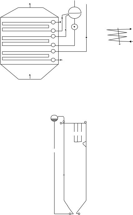
72 |
Steam Generators and Waste Heat Boilers: For Process and Plant Engineers |
To stack |
Drum |
|
|
|
|
|
Water in |
|
|
Flue gases |
Steam out |
|
|
|
Economizer |
Pump |
|
|
|
|
Evaporator |
|
Feed water in |
|
|
|
Once through |
SH steam |
boiler |
Superheater
GT exhaust in
Forced circulation HRSG
is is a forced circulation system generally seen with horizontal evaporator tubes. A circulation pump is used to suck water from the drum and ensure its •ow through the evaporator tubes back into the drum. e pump capacity determines the CR, which can vary from three to eight depending on
the designer’s choice.
(c)
Riser
Drum
Superheater
Downcomer
Furnace
(d)
FIGURE 2.13 (Continued)
(c) Forced circulation system. (d) High-pressure boiler with external downcomers and risers.
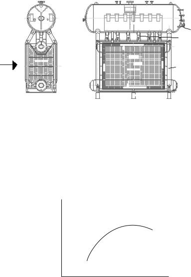
Steam Generator Furnace Design |
73 |
Feed water
Riser pipes
Gas in
Downcomer pipes
Elevated drum water tube boiler
Feed water enters the drum from the boiler feed pump or from an economizer. is mixes with the water
from the evaporator tubes and the mixture •ows down the downcomer pipes to the bottom of the evaporator
tubes. Steam–water mixture is generated in the evporator tubes which is separated into water and steam and then the saturated steam leaves the drum. e amount of steam–water mixture circulated in the system divided by the steam generated is called the circulation ratio. CR is established by an iterative process. It can vary from 5 to 40
depending upon so many variables discussed.
(e)
Circulation ow, kg/h
(f) |
Load, % |
|
FIGURE 2.13 (Continued)
(e) Cross-flow boiler with elevated drum and external downcomers and risers. (f) Load versus circulation rate.
gases, may be generating more than 70% of the steam in the boiler banks, and hence, there is a need to do a section-by-section analysis.
In many package boilers, the drum is integral as shown in Figure 2.3a. In these boilers, external downcomers are not used. Portion of the bank tubes act as downcomers. These are typically located at the cooler end of the bank tubes, where the energy transfer to the tubes is minimal, and hence, the water enthalpy pickup is not much. The number of heated downcomers is obtained through circulation calculations to ensure that the enthalpy pickup is not significant. If tubes that are in very high gas temperature zone are
74 |
Steam Generators and Waste Heat Boilers: For Process and Plant Engineers |
selected as downcomers, then due to the high enthalpy pickup, steam can be generated in these tubes, which will hinder flow of cooler water down the tubes. Due to this formation of steam bubbles, water flow through downcomers is disrupted, affecting the circulation process. Evaporator tubes have failed through overheating due to poor circulation even though the heat flux was low. It is also likely that stagnation of flow can occur as these tubes can neither act as risers. Hence, over a period of time, these tubes reach the flue gas temperatures and can get overheated and fail. The author has seen these issues in some plants. Correction may be implemented through proper baffling inside the drum to ensure that only the tubes located in the cool gas region act as downcomers. If downcomers are properly selected, the cool water flowing down the tubes will have a higher density than the hotter steam–water mixture in the riser tubes, which ensures good circulation.
The quality of steam at the exit of the riser for a CR of 10 will be 0.1, or 10% is the wetness of steam in the mixture. Low-pressure boilers (up to 40 barg) may have a CR ranging from 15 to 40, while higher-pressure units may have a CR ranging from 5 to 15. This is determined by the balance between the available head and the losses in the circulation system. In a forced circulation system, a circulating pump takes water from the drum and forces it through the evaporator tubes. In these types of boilers (Figure 2.13c), one may predetermine the CR, depending on experience. Since pumps assure that circulation will occur, a low value of 3–8 may be used depending on the cost of pump and electricity. Note that the operating costs are higher if circulating pumps are used.
Circulation calculations or determination of CR in each circuit is not the end in itself. A CR of 10 or 15 does not mean much unless factors such as heat flux inside the tubes, mass flow inside the tubes, steam pressure, and orientation of evaporator tubes whether horizontal or vertical are considered.
In evaporator tube as shown in Figure 2.13a, bubbles start forming as the water gets heated in the risers. If the heat flux is below the DNB limits, bubble formation is not intense, and tubes will be wetted by the water film ensuring cool tubes. The tube wall temperature in a normal riser tube is expected to be 5°C–15°C above saturation temperature. If tubeside deposits are present due to poor water chemistry, then this temperature can shoot up. If the heat flux suddenly increases to critical limits, then the vapor formation is so intense that the film of vapor forms around the periphery of the tubes increasing the tube temperature significantly causing it to fail. As the vapor film has a much lower heat transfer coefficient compared to water, it will not be able to cool the tubes effectively, and hence, the temperature rise will be significant. Hence, CR has to be looked at along with the several other variables discussed to find out if the possibility of overheating exists.
As part of circulation study, one has to check the actual heat flux inside the tubes with the allowable heat flux for which correlations are available in the literature. There must be sufficient margin between the two to avoid what is called DNB condition. The heat flux inside the tubes at DNB conditions is called the CHF. DNB checks are initiated when heat fluxes exceed 600–700 kW/m2 (190–212,000 Btu/ft2 h) for steam pressures less than140 barg (2,030 psig).. There are correlations in the literature for CHF depending tube diameter, mass flow inside the tubes, pressure, and tube orientation. Note that heat flux in a plain tube is much lower than in a finned tube. Hence, one should be careful in designing evaporators or once-through steam generators in a fired HRSG; evaporators are designed with varying fin density in each row so the high gas temperature regions have low heat flux and vice versa. The fin density varies from, say, 2 in high gas temperature region to, say, 5 in a much cooler gas temperature region.
It may be noted that a circulation pump is not always required with horizontal tube evaporators. Natural circulation system as discussed in Chapter 4 for a steel mill waste

Steam Generator Furnace Design |
75 |
heat boiler was designed without circulating pumps. This evaporator had plain tubes, and hence, the heat flux inside the tubes was not high. The streams and the location of the drum should be selected with care, and circulations should be done to ensure that the fluid velocity inside the tubes is reasonably high and will not cause stagnation or separation of flow. The heat flux also is an important variable. With finned tubes, the heat flux inside the tubes particularly if the boiler is fired will be high, and hence, circulation pumps provide some safety factor.
While designing a steam generator, the sizing calculations are first performed followed by off-design calculations as discussed in Chapter 3 and Appendix A. The maximum load conditions or the highest furnace heat flux cases are generally chosen for circulation study. The energy absorbed in each section of the boiler such as furnace front and rear walls, side walls, and bank tubes is evaluated along with steam generation in each section. For example, the furnace duty may be estimated as shown earlier. Then based on the average heat flux in the furnace and considering variations in heat flux along the flame length, one can assign duty to each section from which the steam flow is estimated. Oil-fired boilers have a higher operating heat flux in the furnace compared to gas-fired boilers as discussed earlier.
Figure 2.9 shows how the furnace gas temperature (and hence the heat flux) varies along the furnace length. The maximum point occurs a short distance away from the burner location and cooling occurs along the furnace length. This fact is also considered while arriving at the estimation of steam generation in each section of the furnace. As one can see, the distribution is subject to many variables, and no clear formula or empirical equation can provide this information. It is generally based on the experience of the boiler supplier and field data of operating units. Losses from two-phase flow must be estimated for performing circulation studies. The next section deals with estimation of various losses.
Thom’s Method for Estimating Losses [3,4]
The circulation calculations balance the static head available with the losses occurring in the steam loop. The downcomer flow is single phase, and hence, the following equation may be used for estimating the pressure loss as discussed in Appendix B.
P = 810 × 10−6 f Lev w2/di5 |
(2.16) |
where, w is the flow in each pipe in kg/s.
The friction loss ΔPf in kPa in the heated riser tube is estimated by the following equation:
ΔP = 38 × 10−12 |
f v |
L G 2 |
r /d |
i |
(2.17) |
f |
f |
i |
3 |
|
where
f is 4× Fanning’s friction factor = Moody’s friction factor
L is the total effective length over which two-phase friction loss occurs, m vf is the specific volume of saturated water, m3/kg
Gi is the tube-side mass velocity, kg/m2 h di is the tube ID, m
r3 is Thom’s friction loss factor (Figure 2.14b)

76 |
Steam Generators and Waste Heat Boilers: For Process and Plant Engineers |
r2
100 |
|
80 |
100 |
|||||
|
90 |
|||||||
70 |
|
|||||||
|
70 |
|
||||||
50 |
|
60 |
|
|||||
40 |
|
50 |
|
|
||||
30 |
|
40 |
|
|
||||
20 |
|
30 |
|
|
||||
10 |
|
20 |
|
|
||||
9 |
|
15 |
|
|
||||
|
|
|
||||||
8 |
|
|
|
|||||
7 |
|
|
|
|
|
|
|
|
6 |
|
10 |
|
|
||||
5 |
|
9 |
|
|
||||
|
|
|||||||
4 |
|
|
|
|
8 |
|
|
|
|
|
7 |
|
|
||||
3 |
|
|
|
|
6 |
|
|
|
|
|
|
|
|||||
2 |
|
5 |
|
|
|
|||
|
|
4 |
|
|
|
|||
|
|
|
||||||
|
|
|
|
|
|
|
||
|
|
3 |
|
|
|
|||
1.00 |
|
|
|
2 |
|
|
|
|
0.9 |
|
|
|
|
|
|
||
|
|
|
|
|||||
0.8 |
|
1.5 |
|
|||||
0.7 |
|
|
||||||
0.6 |
|
|
|
|
|
|
|
|
|
1.0 |
|
||||||
0.5 |
|
|
||||||
0.4 |
|
|
|
|
|
|
|
|
0.3 |
|
|
|
|
|
|
|
|
0.2 |
|
|
|
|
|
|
|
|
0.10 |
|
|
|
|
|
|
|
|
|
200 |
|||||||
(a)
Dr |
||
|
y |
|
|
|
saturate |
|
|
d |
|
|
steam |
|
|
outle |
|
|
t |
% |
|
|
steam |
by |
ma |
|
||
|
|
|
|
|
ss |
|
|
at |
|
|
outlet |
r3
40
70
30 50
2040
30
20
10 15
7 10
5 7
4
5
34
3
2 2
1.51.5
Dr y
saturate d
steam at
outle t
% steamby
ma ss at outlet
|
|
|
|
|
|
1 |
Water |
|
|
|
|
|
300 |
400 500 |
|
|
|
|
1200 0 |
|
|
|
|
||
700 |
1000 |
2000 |
3000 |
300 |
500 |
600 |
1000 |
2000 |
3000 |
|||
Operating pressure, psia |
(b) |
|
|
Operating pressure, psia |
|
|
||||||
|
|
1.0 |
0 |
Water |
|
|
|
|
|
|
|
|
|
|
0.9 |
1 |
|
|
|
|
|
|
|
|
|
|
|
0.8 |
|
|
|
|
|
|
|
|
|
|
|
|
0.7 |
2 |
|
|
|
|
|
|
|
|
|
|
|
0.6 |
|
|
|
|
|
|
|
|
|
|
0.55
|
|
|
|
|
t |
|
|
|
0.4 |
10 |
|
|
|
atoutle |
|
|
|
|
|
|
ss |
|
|
|
||
0.3 |
|
|
ma |
|
|
|
|
|
|
|
by |
|
|
|
|
|
|
r |
20 |
steam |
|
|
|
|
|
|
% |
atinlet) |
|
|
t |
|
|||
4 |
|
|
|
|
|
|
||
0.2 |
30 |
(Xm=0 |
|
steam |
at |
outle |
|
|
|
|
|
||||||
|
40 |
|
|
|
|
|
|
|
|
|
|
|
d |
|
|
|
|
|
50 |
|
|
saturate |
|
|
|
|
0.10 |
70 |
|
y |
|
|
|
|
|
|
Dr |
|
|
|
|
|
||
|
100 |
|
|
|
|
|
|
|
0.05 |
200 |
|
500 |
|
1000 |
|
2000 |
3000 |
|
|
|
|
|||||
(c)Operating pressure, psia
FIGURE 2.14
Thom’s multiplication factor for (a) acceleration loss and (b) friction loss. (c) Thom’s two-phase multiplication factor for gravity loss.
Steam Generator Furnace Design |
|
|
|
|
|
|
77 |
||||||
|
TABLE 2.3 |
|
|
|
|
|
|
|
|
|
|
|
|
|
Two-Phase Pressure Drop Correlations |
|
|
|
|
|
|
|
|
||||
|
|
|
|
|
|
|
|
|
|
|
|
||
|
SI |
|
|
|
|
British |
Metric |
|
|
|
|
||
|
|
|
|
|
|
|
|
|
|
|
|||
|
ΔP |
= 7.65 × 10⁻¹¹ v Gi2r |
2 |
1.664 × 10⁻¹¹ v G2r |
2 |
ΔP = 7.8 × 10⁻¹³ |
v Gi2r |
2 |
|
|
|||
|
a |
|
|
|
f |
a |
f |
|
|
|
|||
|
ΔP |
= 38 × 10−12 fv LG |
2r /d |
4 × 10⁻¹⁰ fv LG2r /d |
ΔP = 0.388 × 10⁻¹² fv |
LG |
2r /d |
||||||
|
f |
f i |
|
3 i |
f |
3 |
i |
f |
f |
|
i |
3 i |
|
|
ΔPg = 0.00981 Lr4/vf |
|
|
0.00695 Lr4/vf |
|
ΔPg = 0.0001 Lr4/vf |
|
|
|
|
|||
|
G, kg/m2 h |
|
|
lb/ft2 h |
|
|
G, kg/m2 h |
|
|
|
|
|
|
|
w, kg/s |
|
|
lb/h |
|
|
w, kg/s |
|
|
|
|
|
|
|
L, m |
|
|
ft |
|
|
L, m |
|
|
|
|
|
|
|
f, Moody’s friction factor |
Fanning friction factor = Moody’s |
f, Moody’s friction factor |
||||||||||
|
|
|
|
|
friction factor/4 |
|
|
|
|
|
|
|
|
|
di, m |
|
|
In |
|
|
di, m |
|
|
|
|
|
|
|
vf, m3/kg |
|
|
ft3/lb |
|
|
m3/kg |
|
|
|
|
|
|
|
ΔP, pressure loss, kPa |
|
|
psi |
|
|
kg/cm2 |
|
|
|
|
|
|
The gravity loss in the heated riser section in kPa is given by |
|
|
|
|
|
|
|||||||
|
|
|
|
|
ΔPg = 0.00981 Lr4/vf |
|
|
|
|
(2.18) |
|||
where
L is the length of the boiling section in m
vf is the specific volume of saturated water, m3/kg
r4 is the multiplication factor for gravity loss (Figure 2.14c)
ΔPa is the acceleration loss in kPa due to change of phase, which is significant at low steam pressures and high mass velocities and is given by
ΔP = 7.65 × 10⁻¹¹ |
v |
Gi2r |
2 |
(2.19) |
a |
f |
|
|
r2 is the acceleration loss multiplication factor as shown in Figure 2.14a.
The correlations are shown in Table 2.3 in all three systems of units.
Circulation Calculations
Circulation calculation in a natural circulation boiler is an iterative process.
1.First, a CR is assumed based on experience and type of steam generator and pressure. For low-pressure boilers (<70 barg), CR could range from 12 to 35, while for higher-pressure units, it can range from 5 to 15. CR = 1/x where x is the steam quality, fraction. Flow through the downcomers, evaporators, and risers is CR x steam generated.
2.The feed water temperature entering the drum should be known from thermal calculations, which should have already been done. This includes the complete boiler performance as illustrated in Chapter 3, furnace calculations, and estimation of energy absorbed in each parallel path such as front wall, rear wall, and side
78 |
Steam Generators and Waste Heat Boilers: For Process and Plant Engineers |
walls. The resistance of each path must also be known. Mixture enthalpy entering the downcomers is calculated through an energy balance around the drum, Figure 2.13a.
hfw + CR × he = hg + CR × hm |
(2.20) |
where hfw, he, hm, and hg are the enthalpy of feed water, steam–water mixture leaving the evaporator, water entering the downcomers, and saturated steam, respectively.
It should be noted that cool water entering the downcomer aids better circulation. If hm is close to or at saturation, then bubbles will be formed in the region near the entry of downcomer pipes, and circulation will be hindered. There may be several downcomers in a boiler each with a different length and pipe size. A flow and pressure balance calculation is done to arrive at the flow in each downcomer and riser.
As the downcomer flow enters the evaporator, it gets heated, and boiling starts after a distance from the bottom of the furnace. This is called the boiling height, Lb.
Lb = L × CR × Ws (hf − hm)/Q |
(2.21) |
(All in consistent units)
hf is the enthalpy of saturated liquid
Q is the energy absorbed in the furnace L is the furnace height
Ws is the steam generated by the boiler
1.The static head available is first estimated. It is typically the distance from the drum water level to the bottom of the furnace; then the following losses are estimated:
2.Losses in the downcomers including entry and exit losses.
3.Losses in the boiling height and two-phase losses such as friction, acceleration, and gravity using Thom’s method or similar well-known two-phase correlations.
4.If there are unheated risers, their losses are estimated. Again there may be several parallel paths with different pipe sizes and lengths. Flow in each parallel path is evaluated by estimating the pressure drop in each path for different flows and ensuring that the pressure drop is the same. This is an iterative process. These calculations are preferably done using a computer program.
5.Loss in drum internals. This is impacted by the presence of cyclones inside the drum for steam separation.
The static head is balanced with various losses, and if they match, the CR assumed is fine; else, another CR is assumed and the calculations are repeated. If there are multiple parallel paths (a D-type boiler has front wall, rear wall, side wall, and boiler bank tubes), then flow and pressure balance calculations are carried out to ensure that the total losses in each parallel path are the same. CR in each parallel path may differ depending on its energy absorbed, tube size used, and resistance to flow.
Once the circulation calculations are done, the flow in each evaporator tube will be known along with the steam quality at its exit. Checks for heat flux in each path and DNB
Steam Generator Furnace Design |
79 |
based on exit quality are then done. The variation of heat flux along flame length and view factors based on tube spacing enter into these calculations. If there is a potential for DNB, then efforts are taken to revise the downcomer and riser system pipe sizes to improve the CR in the boiler; else, the heat flux in the furnace has to be reduced, and the boiler design is redone. Based on experience and field data, one should be able to arrive at a good system considering these concerns.
Example 2.9
A waste heat boiler similar to the system shown in Figure 2.13a has the following data: steam pressure = 55.1 barg (800 psig). Static head available (from drum centerline to bottom of evaporator bundle) = 8 m. Steam drum is located far away from the evaporator, which is generating 58 t/h of steam; feed water temperature is 120°C.
Two downcomers of ID 285 mm and length 14 m and with six 90° bends are feeding the evaporator with two risers of ID 317 mm and of length 11 m with five bends are feeding drum. The evaporator bundle is 6 m high and has 420-44 mm ID tubes. Determine the approximate CR in the evaporator. Drum internals loss = 352 kg/m2.
Solution
First, the energy balance is performed in the drum assuming a CR. Say CR = 11.
At 55.1 bar, from steam tables, vg = 0.035 and vf = 0.0013 m3/kg. Enthalpy of feed water hf = 121.2 kcal/kg, enthalpy of saturated steam hg = 666.1 kcal/kg, and saturated water hl = 284.27 kcal/kg. Saturated steam temperature = 271°C.
Assume CR = 11. Mixture enthalpy leaving the drum he = 0.0909 × 666.1 + 0.9091 × 284.27 = 319 kcal/kg. From energy balance in the drum,
11 × 319 + 121.2 = 666.1 + 11hm or hm = 269.5 kcal/kg. From steam tables, this corresponds to 259°C and vm = 0.001271 m3/kg. Hence, the water will start boiling after some distance from the bottom as the saturated steam temperature is 271°C.
1.Static head available = 8/.001271 = 6294 kg/m2.
2.To compute the losses in downcomers, the velocity of water in downcomer
must be known. Vdc = 1.246wvm/di2 (see Appendix B for formula for velocity inside tubes). Flow in each downcomer w = 11 × 58,000/2/3,600 = 88.6 kg/s.
Then Vdc = 1.246 × 88.6 × 0.001271/0.285/0.285 = 1.73 m/s. Velocity head VH = V2/(2gvm) = 1.73 × 1.73/2/9.8/0.001271 = 120 kg/m2 (g = 9.8 m/s2). The entrance plus exit loss in downcomer = 1.5VH = 180 kg/m2.
Equivalent length of downcomer (see Table B.7 for equivalent length of 90° bends) = 11 + 32 × 0.285 × 6 = 54.7 m. Total equivalent length = 11 + 54.7 = 65.7 m
Friction loss in downcomer = 810 × 10−6fLevmw2/di5 = 810 × 10−6 × 0.012 × 66 × 0.001271 × 88.6 × 88.6/0.2855 = 3.4 kPa = 347 kg/m2
Boiling height is then determined. Lb = CR × L × (hl − hm)/(hv − hf) = 11 × 6(284.27 − 269.5)/(666.1 − 121.2) = 1.79 m. Note that a large boiling length reduces the CR as the net thermal head for forcing the two-phase flow through the evaporator tubes reduces. A higher feed water temperature entering the drum helps but not close to saturation as that will hinder flow through downcomer tubes in case the downcomer tubes are partly heated.
The gravity loss in the boiling length before start of boiling = 1.79/0.001285 = 1393 kg/m2 (an average specific volume between that of saturated liquid and the colder water entering the evaporator is taken).
The gravity loss in the evaporator section is ΔPg = 0.00981Lr4/vf. r4 from Figure 2.14c = 0.65. ΔPg = 0.00981 × (6 − 1.79) × 0.65/.0013 = 20.62 kPa = 2104 kg/m2.
80 |
Steam Generators and Waste Heat Boilers: For Process and Plant Engineers |
The friction loss may be shown to be very small due to the large number of tubes used. r3 = 2.3 from Figure 2.14b. ΔPf = 38 × 10−12 f vl L Gi2 r3/di
G = 58,000 × 11 × 4/(3.14 × 420 × .0442) = 999,531 kg/m2 h
ΔPf = 38 × 10−12 × 0.02 × 0.0013 × 4.21 × (999,531)2 × 2.3/.044 = 0.217 kPa = 22 kg/m2 Average mass flow in each tube = 58,000 × 11/420/3,600 = 0.42 kg/s
Friction loss in the single-phase heated section = ΔPf = 810 × 10−6 × 0.02 × 1.79 × 0.001285 × 0.422/0.0445 = 0.04 kPa = 4 kg/m2
At entrance to evaporator bundle, velocity = 1.246 × 0.42 × 0.001271/0.0442 = 0.34 m/s Specific volume of steam mixture at evaporator exit = 0.0909 × 0.035 + (1 − 0.0909) ×
0.0013 = 0.004363 m3/kg (1/CR = 0.0909)
Entrance loss = 0.5VH = 0.5 × 0.34 × 0.34/2/9.8/.001271 = 2.32 kg/m2
Exit velocity = 1.246 × 0.42 × 0.004363/.044/.044 = 1.179 m/s. Exit loss = 1 VH = 1.179 × 1.179/2/9.8/.004363 = 16.3 kg/m2
Acceleration loss ΔPa = 7.65 × 10⁻¹¹ vf Gi2r2
r2 = 1.45 from Figure 2.14a. ΔPa = 7.65 × 10−11 × 0.0013 × (999,531)2 × 1.45 = 0.14 kPa = 14 kg/m2 Velocity of steam in riser pipe = 1.246 × 88.6 × 0.004363/0.3172 = 4.79 m/s
Inlet and exit loss = 1.5VH = 1.5 × 4.792 × 4.79/(2 × 9.8 × 0.004363) = 402 kg/m2 Le = equivalent length = 11 + 5 × 32 × 0.317 = 61.7 m
Friction loss = 810 × 10−6 fLeveW2/di5 = 810 × 10−6 × 0.011 × 61.7 × 0.004363 × 88.6 × 88.6/0.3175 = 0.095 kPa = 952 kg/m2 (using homogeneous model)
The difference in height between the drum centerline and the evaporator header is about 2 m. The gravity head in the riser pipe = 2/0.004363 = 458 kg/m2. (Using the relation between slip factor, void fraction, and quality, one can come up with more accurate estimation of gravity loss.)
Summary of Losses
1.Downcomer inlet and exit loss = 180 kg/m2
2.Downcomer friction loss = 347 kg/m2
3.Gravity loss in evaporator section = 1393 + 2104 = 3497 kg/m2
4.Friction loss in evaporator length = 22 + 4 + 2 + 16 = 44 kg/m2
5.Acceleration loss = 14 kg/m2
6.Riser inlet and exit loss = 402 kg/m2
7.Riser friction loss = 952 kg/m2
8.Unheated riser pipe gravity head = 458 kg/m2
9.Drum internals loss = 352 kg/m2 (0.5 psi is a conservative estimate)
Total losses = 6246 kg/m2. Available head = 6294 kg/m2. Hence CR is in the range of 11. A computer program is helpful in performing these calculations more accurately. One can consider variation in steam generation in individual paths, differences in downcomer and riser sizes and lengths of parallel paths, effect of feed water temperature, and so on. Also this is a tedious calculation as we have to assume a CR and perform all these calculations and check if available head matches the losses. If not, another CR is assumed, and these calculations are repeated. For the earlier illustration, a CR close to the computer-calculated value was chosen. The manual calculation showed a simplistic model for illustration. The first few rows of tubes of evaporator will be generating more steam, and hence, the CR in these tubes could be slightly lower. If risers or downcomers with different lengths are used, the flow in each could vary. One should then check the heat flux in each section and ensure that the CHF levels are not reached.
Steam Generator Furnace Design |
81 |
Example 2.10
Pressure drop in two-phase flow may be estimated using the average specific volume as well as by using Thom’s method. Let us compare the difference. In a once-through boiler, 15,000 kg/h of two-phase mixture at 105.5 kg/cm2 a absolute pressure with exit quality of 80% flows inside a pipe of inner diameter 50 mm. For an effective length of 50 m, compute the friction loss using Thom’s method and homogeneous model using average specific volume of mixture.
Solution
From steam tables, vg = 0.01728 m3/kg, vf = 0.001469 m3/kg
Mixture-specific volume at exit of boiler = 0.8 × 0.01728 + 0.2 × 0.001469 = 0.0141 m3/kg Average specific volume in the boiler = (0.001469 + 0.0141)/2 = 0.007785 m3/kg
w = 15,000/3,600 = 4.17 kg/s. r3 from Figure 2.14b = 5.7
ΔP = 810 × 10−6 × 0.02 × 50 × 4.172 × 0.007785/0.055 = 354 kPa = 3.6 kg/cm2 [51 psi] P(Thom) = 38 × 10−12 × 0.02 × 0.001469 × (15,000 × 4/3.14 × 0.05 × 0.05)2 × 5.7 × 50/0.05 =
371 kPa = 3.79 kg/cm2 [54 psi]
Hence, in the absence of Thom’s curves, one may estimate the two-phase friction loss using an average specific volume in the boiling section.
Example 2.11
A simplified version of circulation calculations for the boiler in Figure 2.13b is shown. The boiler is a natural gas–fired D-type boiler with external drum, downcomers, and risers and generates 190 t/h of saturated steam at 40 kg/cm2 a. Energy balance calculations were done, and the energy transferred in each section of furnace such as D tubes, front wall, rear wall, and the convection bank tubes was estimated using a thermal performance program. The steam generation in each section was estimated. Then, the geometric data for the circulation system, namely, the number of external downcomers, risers, and lengths of each section were inputted in a circulation program, results of which are shown in Table 2.4.
The front and rear walls have a CR of about 20, while the D-tubes have a CR of about 12 and the bank tubes about 19 giving an overall average CR of 16.8.The calculations can be more detailed with split-up of the bank tubes into several sections. However, this is only for illustrating that CR varies in each circuit depending on its resistance to flow and steam generation.
Natural circulation is adopted in small and large boilers up to a pressure of about 165 barg. Beyond this, forced circulation is required as the density difference between steam and water decreases.
Circulation Flow versus Load
The amount of flow circulated through a steam generator typically shows a trend shown in Figure 2.13f. As the load increases, the heat flux in various parts of the evaporator increases, and hence, the difference in density between the cooler downcomer water mixture and the flow in the evaporator tubes increases increasing the circulation flow through the system. However, beyond the maximum load, the resistance offered by the riser circuits and drum internals dominates and reduces the flow circulating through the system. If the CR at 100% load is, say, 15, then at 80% load, it could be 17, and at 120% load, it could be 11. At 100% load, the mixture flow = 15 × 100 = 1500. At 80% load, 80 × 17 = 1360, and at 120% load, 120 × 11 = 1320. Overloading a steam generator is not recommended for this reason, and critical circuits must be evaluated for DNB concerns.

82 |
|
Steam Generators and Waste Heat Boilers: For Process and Plant Engineers |
||||||||
TABLE 2.4 |
|
|
|
|
|
|
|
|
|
|
Results of Circulation Calculations |
|
|
|
|
|
|
||||
|
|
|
|
|
|
|
||||
Steam Pressure |
|
40 |
Section |
|
Steam kg/h |
CR |
||||
|
|
|
|
|
|
|
|
|
||
Sat temperature |
|
249 |
|
Front wall |
|
5,300 |
|
20 |
||
Feed water temp |
|
194 |
|
Rear wall |
|
2,830 |
|
20.5 |
||
Sp vol steam |
|
0.0508 |
D tubes |
|
58,300 |
|
12.1 |
|||
Sp vol water |
|
0.0012 |
Bank tubes |
|
127,000 |
|
19.1 |
|||
Average CR |
|
16.8 |
|
Units |
|
|
|
|
||
Total static head |
|
7.80 |
|
Flow |
|
kg/h |
|
|
||
Total static head |
|
0.63 |
|
Length |
|
m |
|
|
||
Downcomer losses |
|
0.10 |
|
Pressure |
|
kg/cm2 a |
|
|
||
Riser losses |
|
0.10 |
|
Press loss |
|
kg/cm2 |
|
|
||
Riser gravity loss |
|
0.11 |
|
Tube dia |
|
mm |
|
|
||
Drum internal loss |
|
0.04 |
|
Velocity |
|
m/s |
|
|
||
Mixture temp |
|
246 |
|
Sp volume |
|
m3/kg |
|
|
||
|
|
|
|
|
|
|
|
|
|
|
Path |
Level |
Sort |
Dia |
Length |
Bends |
Flow |
Velocity |
No tubes |
Pr. drop |
Item |
|
|
|
|
|
|
|
|
|
|
|
1 |
1 |
1 |
289 |
8 |
3 |
3,246,264 |
2.81 |
6 |
0.10 |
dc |
1 |
1 |
1 |
289 |
1.22 |
0 |
3,246,264 |
7.08 |
8 |
0.10 |
riser |
Steam |
Quality |
Accln |
Gravity |
Friction |
Total flow |
Tubes |
Tube ID |
Boil ht. |
Length |
CR |
|
|
|
|
|
|
|
|
|
|
|
5,300 |
0.05 |
0.002 |
0.29 |
0.01 |
106,000 |
30 |
56.00 |
4.9 |
4.90 |
20.0 |
2,630 |
0.049 |
0.001 |
0.292 |
0.002 |
53,893 |
30 |
56.00 |
4.9 |
4.90 |
20.5 |
58,300 |
0.082 |
0.01 |
0.246 |
0.046 |
707,524 |
120 |
56.00 |
4.9 |
8.50 |
12.1 |
127,000 |
0.052 |
0.001 |
0.286 |
0.007 |
2,423,664 |
1320 |
45.00 |
4.9 |
4.90 |
19.1 |
|
|
|
|
|
|
|
|
|
|
|
Flow Stratification in Horizontal Tubes
With horizontal tubes in two-phase flow, one has to also check if flow stagnation is likely. Froude number is an indicator of inertial forces to gravity forces, and if it is above 0.04, flow separation is unlikely. Froude number F = G2/ρ2gd where G = mass flow inside the tubes (liquid only), kg/m2 s. ρ = density of liquid (807 kg/m3), g = acceleration due to gravity (9.8 m/s2), and d = tube inner diameter (0.026 m).
Correlations for CHF (Critical Heat Flux) and Allowable Steam Quality
One may obtain the heat flux given the steam quality, mass flow inside tubes, steam pressure, and tube inner diameter or conversely obtain the allowable steam quality given a heat flux. There are several correlations for CHF, and the Kastner correlation [4] is one of them. It gives the allowable quality at any mass flow and heat flux and steam pressure.
For 0.49 < P < 2.94 MPa [5] |
|
|
|
x = 25.6(1000q)−0.125 |
m(−0.33)(1000d )−0.07 e0.1715P |
(2.22) |
|
c |
|
i |
|
For 2.94 < P < 9.8 MPa |
|
|
|
x = 46(1000q)−0.125 |
m(−0.33)(1000d )−0.07 e−0.0255P |
(2.23) |
|
c |
|
i |
|

Steam Generator Furnace Design |
|
83 |
For 9.8 < P < 19.6 MPa |
|
|
x = 76.6(1000q)−0.125 |
m(−0.33)(1000d )−0.07 e−0.0795P |
(2.24) |
c |
i |
|
(Steam pressure P in MPa, di in m, q in kW/m2, m in kg/m2s)
Example 2.12
Steam is generated at 50 bara in a boiler using 40 mm tubes. Heat flux is 300 kW/m2. Mass velocity of steam water mixture inside tubes is 750 kg/m2 s. Determine the maximum allowable quality or CR to avoid DNB conditions.
xc = 46(1000q)−0.125 m(−0.33)(1000di) −0.07 e−0.0255P
P = 50 bara = 5 MPa, m = 750 kg/m2 s, di = .040 m, q = 300 kW/m2.
xc = 46 × (300,000)−0.125 750−0.33 40−0.07 e−0.0255×5 = 0.73 or 73% allowable quality or a CR of 1.37 minimum. CR in practice will be much higher than this, and hence, this heat flux is acceptable.
Macbeth correlation gives the CHF, given the other variables, and takes the following form:
qc = 0.5025 hfg di−0.1 (Gi)0.51 (1 − x) |
(2.25) |
where
qc = CHF, kW/m2
x is the steam quality, fraction di is the tube ID, m
Gi is the mass velocity, kg/m2 s
Example 2.13
If G = 816.7 kg/m2s, x = 0.2, di = 0.0381 m, and P = 6.9 MPa (hfg = 361.1 kcal/kg), then qc = 0.5025 × 361.1 × (0.0381)(−0.1) × 816.70.51 × 0.8 = 6150 kW/m2
This being a theoretical correlation does not account for tube-side fouling, and the actual value of CHF could be 20%–30% of this.
Groeneveld’s lookup tables are also used to check for CHF. Table 2.5 shows an extract from 1996 tables.
TABLE 2.5
Groeneveld’s Lookup Tables for CHF in kW/m2 for 8 mm Tubes
Pressure, kPa |
G, kg/m2 s |
X = 0.2 |
0.4 |
0.6 |
0.8 |
3000 |
500 |
5660 |
3392 |
2745 |
1320 |
|
1000 |
5620 |
3079 |
1925 |
830 |
|
1500 |
5043 |
2691 |
1080 |
499 |
|
2000 |
4507 |
2279 |
608 |
330 |
5000 |
500 |
5178 |
3975 |
3040 |
1769 |
|
1000 |
4957 |
3447 |
2066 |
1034 |
|
1500 |
4530 |
2983 |
1194 |
899 |
|
2000 |
3984 |
2557 |
668 |
650 |
Source: IAEA April 2001 report, Thermo-hydraulic relationships for advanced water cooled reactors, IAEA-TECDOC-1203.
Note: P in kPa, G in kg/m2 s, CHF in kW/m2. Use a correction factor of 0.79 for tube ID > 16 mm. This table is based on a tube ID of 8 mm. For diameter above 16 mm, use a correction factor of 0.79.

84 |
Steam Generators and Waste Heat Boilers: For Process and Plant Engineers |
Example 2.14
At 50 barg and with 1000 kg/m2 s mass velocity and 40 mm tube ID and quality = 0.2, the CHF = 4957 × 0.79 = 3916 kW/m2
Though there are several correlations for CHF, many have been developed in laboratories under controlled conditions. They may show different CHF values for the same steam parameters and tube geometry. Hence, charts such as Figure 2.15 developed by boiler firms have more practical value as the results are backed by operation of steam generators [6].
|
40 |
|
|
30 |
|
weight% |
20 |
|
10 |
||
|
||
Quality, |
0 |
|
13 |
||
|
||
|
–10 |
|
|
–20 |
(a) –30
1.100,000(0.32) 2.150,000(0.47) 3.200,000(0.63) 4.250,000(0.79) |
Btu/ft2h (MW/m2) |
|||||
|
|
|
|
1 |
|
|
|
|
|
|
2 |
|
|
|
|
|
|
3 |
|
|
|
|
|
|
4 |
|
|
14 |
15 |
16 |
17 |
18 |
19 |
20 |
|
|
Pressure, MPa |
|
|
|
|
Steam quality vs. critical heat flux
|
|
|
e number on each curve |
|
|
|
|
|
|
|
|
|
||||||||
|
|
|
indicates heat flux as |
|
|
|
|
|
|
|
|
|
||||||||
|
1400 |
|
Btu/ft2h of internal |
|
|
|
|
|
|
|
|
|
||||||||
|
|
|
Tube surface. |
|
|
|
|
|
|
|
|
|
|
|
|
|||||
|
1200 |
|
|
|
|
|
|
|
200,000 |
|
|
|
|
|
|
|
|
|
||
|
|
|
|
|
|
|
|
|
|
|
|
|
|
|
|
|
||||
h |
1000 |
|
|
|
|
|
|
|
|
|
|
|
|
|
|
|
|
|||
|
|
|
|
|
|
|
|
|
|
|
|
|
|
|
|
|
|
|
||
|
|
|
|
|
|
|
|
|
|
|
|
|
|
|
|
|
|
|
|
|
2 |
|
|
|
|
|
|
|
|
100,000 |
|
|
|
|
|
|
|
|
|||
lb/ft |
|
|
|
|
|
|
|
|
|
|
|
|
|
|
|
|
||||
|
|
|
|
|
|
|
|
|
|
|
|
|
|
|
|
|
|
|
|
|
velocity, |
800 |
|
Safe |
Unsafe |
|
|
|
|
|
|
|
|
|
|
|
|
||||
|
|
|
|
|
|
|
|
|
|
|
|
|
||||||||
|
|
|
|
|
|
|
|
|
|
|
|
|
|
|
|
|
||||
|
|
|
|
|
|
|
|
|
|
|
|
|
|
|
|
|
|
|||
Mass |
600 |
|
|
|
|
Safe |
|
|
Unsafe |
|
|
|
|
|
|
|||||
|
|
|
|
|
|
|
|
|
|
|
|
|||||||||
|
|
|
|
|
|
|
|
|
|
|
|
|
|
|
|
|
||||
|
|
|
|
|
|
|
|
|
|
|
|
|
|
|
|
|
|
|||
|
400 |
|
|
|
|
|
|
|
|
|
|
|
|
|
|
|
|
|
|
|
|
|
|
|
|
|
|
|
|
|
|
|
|
|
|
|
|
|
|
|
|
|
200 |
|
|
|
|
|
|
|
|
|
A |
|
|
|
|
|
|
B |
||
|
|
|
|
|
|
|
|
|
|
|
|
|
|
|
|
|||||
|
0 |
|
|
|
|
|
|
|
|
|
|
|
|
|
|
|
|
|
|
|
|
|
|
0 |
10 |
20 |
30 |
40 |
50 |
||||||||||||
(b) |
|
|
|
|
|
Quality, % steam by weight |
|
|
|
|
|
|
||||||||
FIGURE 2.15
(a) Allowable steam quality as a function of heat flux Btu/ft2 h (MW/m2) and steam pressure. (b) Allowable quality for nucleate boiling at 2700 psia. (From Babcock and Wilcox, Steam: Its Generation and Use, 38th edn., B&W, Barlerton, OH, 1992.)

Steam Generator Furnace Design |
85 |
Circulation Problems
The common problem in boiler circulation system is that the downcomer tubes are not properly located or shielded from hot flue gas. If located in the hot gas zone, steam bubbles are likely to be formed at the downcomer inlet preventing the flow of cold water to the bottom of the boiler for circulation. This generally happens through improper baffling inside the drum. The boiler designer may think that the tubes are acting as downcomers, while due to improper baffling, they may be acting as risers. Sometimes, the head is inadequate to ensure flow as downcomers, and hence, stratification occurs with steam bubble formation at downcomer inlet resulting in the stagnation of flow. The tubes can then reach the flue gas temperature and fail even though they may be in 500°C–600°C gas temperature region and the average heat flux in the convection bank is very low, well below the DNB limits. So DNB is not the problem but vapor formation, stratification, and overheating of tubes, which are neither capable of acting as downcomers or risers.
High feed water temperature close to saturation temperature or steaming water entering the drum from the economizer is also a concern. If one computes the mixture enthalpy entering the downcomers, he may find it above saturated water enthalpy or above saturation temperature. The bubble formation at the downcomer inlet prevents water flow to the bottom of the boiler for creating a circulation pattern.
Guidelines for Good Circulation System Design
The following are the guidelines used while designing the downcomer system in a package boiler.
1.The designated downcomer tubes should be located at the coolest gas temperature region; that is where the flue gases make a turn to the economizer. If they are located in a high gas temperature region, the enthalpy absorbed by these tubes can be high, resulting in steam bubble formation inside the tubes, which can hinder downward flow of water and hence the circulation process. Formation of steam does two negative things. It decreases the density of the water in the downcomer, which in turn reduces the available head for circulation and also physically prevents the free flow of downcomer water. So locating downcomers in hot gas zones should be avoided. If inevitable, then the downcomers must be insulated.
2.The gas temperature entering the downcomers should be as low as possible to ensure that even if stagnation occurs, the tubes will not be overheated. A good value is less than 450°C at full load.
3.Belly pans are used to collect steam from risers, and all the water for circulation is allowed to flow from drum normal level through the downcomer tubes. Design velocity chosen for downcomer flow is generally in the range of 1–3 m/s at full load.
4.Proper baffling to be done inside the drum to ensure that tubes, which are supposed to be risers, are inside the belly pan area (see Figure 6.10). This provides these tubes an additional head for circulation. (Density of steam–water mixture in the baffle space of belly pan is lower than the water in the drum; also the static head equivalent to the radius of the drum less the belly pan height is available for

86 |
Steam Generators and Waste Heat Boilers: For Process and Plant Engineers |
circulation process.) If, say, the average CR is 16 (steam quality x = 1/CR = 0.055) in the boiler, the specific volume of the mixture = 0.055 × 0.0435 + 0.945 × 0.00125 = 0.00356 m3/lb, where 0.0435 and 0.00125 are the specific volumes of saturated steam and water, respectively, at 46 bara drum pressure. Hence, the density of the mixture = 1/0.00356 = 281 kg/m3. Assume that the normal water level is at 600 mm in the drum and the belly pan height is 125 mm, then the extra head available for the baffled tubes is (0.600 − 0.125) × 281 = 133 kg/m2, which helps a lot considering that the net head for circulation is in the order of about 3500 kg/m2. So riser tubes should be under the belly pan. Tubes acting as risers in the water-filled region will have difficulty in circulating as this additional head is not available.
5.It is very important that downcomers do not take suction from locations in drum where vaporization or heat flux is intense resulting in sucking of bubbles into downcomers. This will interfere with circulation and also prevent a normal downcomer from acting as a downcomer. In large waste heat boilers, a vortex breaker is provided at the suction line to break up these bubbles.
6.Swaging of tubes inside drums is better avoided as it adds to the flow resistance and impacts circulation. Also, it adds to two-phase flow instabilities. Resistance to flow at the riser end should be avoided, while resistance at downcomer inlet or feed water inlet in once-through boilers improves the stability of two-phase flow as discussed in Chapter 6.
References
1.V. Ganapathy, Industrial Boilers and HRSGs, CRC Press, Boca Raton, FL, 2001, p112.
2.V. Ganapathy, Applied Heat Transfer, Pennwell Books, Tulsa, OK, 1982, p60.
3.V. Ganapathy, Boiler circulation calculations, Hydrocarbon Processing, January 1998, p100.
4.J.R.S. Thom, Prediction of pressure drop during forced circulation boiling of water, International Journal of Heat Transfer, 7, 709–724, 1964.
5.D. Tucakovic et al., Thermal hydraulics of evaporating tubes in the forced circulation loop of a steam boiler, FME Transaction, 36, 1, 2008.
6.Babcock and Wilcox, Steam: Its Generation and Use, 38th edn., Published by B&W, Barlerton, Ohio, 1992.
3
Steam Generators
Introduction
Oiland gas-fired steam generators or boilers as they are often called form an essential part of any power plant or cogeneration system. The steam-based Rankine cycle has been synonymous with power generation for centuries. Though the steam parameters such as pressure and temperature have been steadily increasing during the last several decades, the function of the boiler remains the same, namely, to generate steam at the desired conditions efficiently and with low operating costs while meeting the local emission regulations. Low-pressure steam is used in cogeneration plants for heating or process applications while high-pressure steam is used for generating power via steam turbines. Boiler capacities have undergone significant changes during the past 50 years. Today oilor gas-fired shop-assembled package boiler generating 100–140 t/h of steam at 100 barg, 500°C, is not uncommon (Figure 3.1). Modular design or elevated steam drum design (Figures 3.2 and 3.3) is also evolving to handle yet larger capacities of about 200 t/h steam, while large forced circulation boilers using treated water from oil wells are finding application in oil field applications (Figure 3.4). Another factor that has introduced significant changes in the design of boilers and associated systems is the stringent emission regulations in various parts of the world requiring CO and NOx control systems such as flue gas recirculation (FGR) or selective catalytic reduction system (SCR) adding to the complexity of the boiler design and layout. High efficiency also remains a goal coupled with low fan power consumption; hence, boiler suppliers are offering both custom-designed boilers, wherever required, and standard boilers. This chapter deals with oiland gas-fired steam generators only and not with solid fuel–fired boilers.
Large Package Boilers
Large boilers in the range of 100–200 t/h capacity were once field erected considering the limitations of local rail or road shipping dimensions. Considering the high cost of site erection, during the last three decades, boiler suppliers have come up with modular designs to minimize the labor cost, field erection, and delivery time by maximizing the work done in the shop.
For larger capacities, in the range of 150–200 t/h modular design, Figure 3.2 is an interesting option. Since shipping dimensions are not limiting the size, the furnace dimensions
87

88 |
Steam Generators and Waste Heat Boilers: For Process and Plant Engineers |
FIGURE 3.1
Large package steam generator. (Courtesy of Cleaver Brooks Inc., Engineered Boiler Systems, Thomasville, GA.)
Modular D-type watertube shown in progress. is is one of two identical units designed to produce 250,000 pph of 500 psig/650°F steam.
FIGURE 3.2
Modular steam generator design. (Courtesy of Cleaver Brooks Inc., Engineered Boiler Systems, Thomasville, GA.)
can be chosen independently based on liberal furnace heat release rates; the width of the convection bank can also be large as it is also shipped separately, and hence, the bank tube spacing or that of the superheater if used in the convection bank can have longer lengths or wider tube spacing to minimize the gas velocity and pressure drop, as a result of which the fan can be made smaller and fan power consumption lower. The steam drum can be integral with the boiler bank tubes or can be shipped separately and assembled in the field.
Another option for large units is the elevated drum unit (Figure 3.3), which shows a 193 t/h boiler generating saturated steam for oil field application. The concept of external

Steam Generators |
89 |
FIGURE 3.3
Elevated drum steam generator for large capacity. (Courtesy of Cleaver Brooks Inc., Engineered Boiler Systems, Thomasville, GA.)
FIGURE 3.4
Large-capacity high-pressure forced circulation steam generator for oil sands application. (Courtesy of Cleaver Brooks Inc., Engineered Boiler Systems, Thomasville, GA.)
drum and circulation system has been widely used in waste heat boilers, and the package boiler industry has started adapting these concepts for the benefit of the end users. Considering the high cost of fuel and electricity, these boilers have been designed with a closed-loop glycol heating system, which offers about 2.5% more efficiency over a typical steam generator with an economizer, which is discussed later. Combining the modular and elevated drum boiler concepts, oiland gas-fired steam generators of capacity 200–300 t/h are viable. With minimum field installation time and lower cost of erection, these recent designs are economically attractive to the end user.

90 |
Steam Generators and Waste Heat Boilers: For Process and Plant Engineers |
Water-Cooled Furnaces
Refractory-lined boilers are becoming a thing of the past, and today’s package boiler has completely water-cooled furnaces as shown in Figure 3.2; the water-cooled furnace design has several advantages over refractory-lined units as discussed in Chapter 2. One advantage of the completely water-cooled furnace design is that it enables quick starting of boilers. In combined cycle plants, one important application of steam generators is to provide steam to the steam turbine glands when steam from the HRSGs is not available. A package steam generator is used as a standby boiler, whose important purpose is to supply steam at a short notice, say, when the gas turbine trips. They are called quick start boilers or standby boilers. A steam-heated coil is inserted in the mud drum, which keeps the boiler always warm; sometimes a small additional burner of capacity 3%–5% of the total burner capacity is kept operating all the time, and the boiler makes a small amount of steam at the operating pressure or close to it. When required, it can be brought on line to the required capacity in less than 1–2 min. A refractory-lined boiler will not be suitable for this type of application.
Major Changes in Boiler Design
Major changes have been introduced in the design of oiland gas-fired steam generators of today. Decades ago, boilers were concerned with only two issues, namely, efficiency and operating cost. Low boiler efficiency meant higher fuel cost, and a large gas pressure drop across heating surfaces meant higher fan power consumption. Each addition of 25 mm wc (1 in wc) pressure drop in a boiler of 45 t/h (100,000 lb/h) capacity results in about 5 kW of additional fan power consumption. The difference in efficiency between 5 and 15% excess air operation on natural gas is about 0.4%. Every 22°C drop in flue gas exit temperature adds 1% to the boiler efficiency. Therefore, steam generators were operating at the lowest possible excess air, say, 5%. The effect of excess air and exit gas temperature on boiler efficiency is shown in Figure 3.5 for natural gas firing. With limits on CO and NOx emissions today, this is no longer possible, and higher excess air rates are used as explained later. The expression, “no NOx, no SOx, and no rocks” aptly describes the direction where boiler systems are headed, namely, emission-governed equipment [1].
Absence of Air Heater
The steam generator configuration has changed in the last few decades. The tubular or regenerative air heater, which was once an integral part of the steam generator, is now replaced by the economizer. Air heaters are rarely used in steam generators where NOx emissions have to be limited. Air heater increases the combustion temperature in the furnace and thus increases the NOx levels adding to the cost of pollution control equipment. With natural gas at 15% excess air, each 55°C (100°F) increase in combustion air temperature increases the flame temperature by about 36°C (65°F). In addition, air heater increases

Steam Generators |
91 |
LHV eciency, %
94 |
|
93 |
|
92 |
10% |
|
|
91 |
|
90 |
30% |
|
|
89 |
|
88 |
|
120 |
140 |
160 |
180 |
200 |
|
|
(Tg –Ta), °C |
|
|
FIGURE 3.5
Effect of excess air and exit gas temperature on boiler efficiency for natural gas firing.
1000
NOx, ppm at 3% O2
100 |
|
|
|
|
|
10 |
|
|
500°F air |
|
|
|
|
Amb. air |
|
|
|
|
|
|
|
|
|
1 |
10 |
20 |
30 |
40 |
50 |
0 |
% FGR
FIGURE 3.6
Effect of air temperature on NOx.
the operating cost as it has a larger gasand air-side pressure drop of about 100–120 mm wc compared to the economizer, which has a nominal pressure drop of only 25–30 mm wc. Figure 3.6 shows the effect of air temperature and FGR on NOx emissions. High air temperature increases NOx significantly, and hence, air temperature is kept at ambient or in some high-efficiency systems at less than 60°C–70°C. Air heaters find application in steam generators burning low heating value fuels or solid fuels where flame stability is improved by using hot air but not in natural gas– or fuel oil–fired steam generators. However, several heat recovery systems use them, and their design and performance aspects are discussed in Chapter 4 on waste heat boilers.
There are a few options for increasing the boiler efficiency without using the conventional air heaters. Higher efficiency is achieved in a package boiler today by using a condensing economizer or a closed-loop glycol or thermic fluid heating and cooling system or a scavenger system or by using a low feed water temperature, which are discussed later.

92 |
Steam Generators and Waste Heat Boilers: For Process and Plant Engineers |
Emissions Affect Steam Generator Designs
Present-day package boilers operate at high excess air (15%–20%) with FGR rates ranging from 0% to 30% to limit CO and NOx. Higher the combustion air temperature, higher the FGR rate to achieve the same level of NOx. If fuels containing hydrogen are fired, the flame temperature is higher compared to natural gas, and hence, more NOx is generated and more FGR is required. Hence, air heating is avoided in oiland gas-fired boilers. The reason for the use of high excess air can be seen from Figure 3.7, which shows that as the excess air increases, the NOx level increases and then drops off. When the excess air is a little above stoichiometric, the flame temperature increases up to a certain level due to good mixing of fuel and air, and hence, the NOx increases; as the excess air increases further, the combustion temperature decreases due to the increased mass flow of air and consequent cooling effect; also at low excess air, the CO formation is high due to poor mixing between the fuel and the air. Hence, 15% excess air and 15–25% FGR are widely used in all gasand oil-fired package boilers instead of 5% excess air a few decades ago. This increases the boiler size by 15%–25% if gas pressure drop has to be limited. A larger economizer is also required to maintain the same stack flue gas temperature and efficiency as the design without FGR.
If SCR is added to lower NOx (Figure 3.8), the evaporator section may have to use a gas bypass system to ensure that the catalyst operates in the optimum range of gas temperatures (350°C–420°C) to guarantee NOx levels adding to the complexity of the boiler construction. Catalysts are available for low gas temperature operation also, which can be located ahead of the economizer or even behind it. The location of the catalyst, whether between the evaporator and the economizer or beyond the economizer, also affects the boiler layout. More information on SCR catalysts and ammonia grid is provided in Chapter 4. Lo-NOx burners also have been developed by boiler suppliers to handle the low emission levels of NOx and CO (Figure 3.9). These may require a minimum furnace cross section to avoid flame impingement and a furnace length different from a standard furnace. Thus, standardization is possible only to a limited extent in large water tube boiler designs. While standard boiler applications find a place in the industry, there are numerous applications where a custom-designed boiler would fit the needs of the end
CO
NOx
0.9 |
1.0 |
1.1 |
1.2 |
1.3 |
1.4 |
Excess air factor
FIGURE 3.7
Typical NOx and CO levels versus excess air.

Steam Generators |
93 |
|
|
|
|
Burner |
|
Economizer |
|
|
|
|
|
|
|
|
|
|
FD fan |
Boiler |
|
||||
Air |
|
|
|
|
|
||
|
|
|
|
|
|||
(a) |
|
|
|
|
|
|
|
|
|
|
|
Damper |
|||
|
FD fan |
|
|
|
|||
Air |
|
|
|
|
Furnace |
||
|
|
|
|
||||
|
|
|
|
|
Convection bank |
||
Ammonia
grid
(b) |
SCR — Economizer |
FIGURE 3.8
Arrangement of (a) FGR and (b) SCR system in package boiler for NOx control.
Dual burner, 600 MMBtu/h
FIGURE 3.9
Low NOx burner. (Courtesy of Cleaver Brooks Inc., Natcom Burners, Thomasville, GA.)
user better and lower the user’s cost of owning the boiler. Plant engineers prefer customdesigned boilers as it lowers the operating costs and saves them money in the long run.
Operators must also consider the risk of operating a boiler near the limits of inflammability when using high FGR rate. Figure 3.10 shows the narrowing between the upper flammability limit and lower ignition limit as FGR increases. Integrating control systems to maintain fuel/air ratios at high FGR rates is difficult because FGR dampens the combustion process to the ragged edges of flammability-flameouts and flame instability. Full metering combustion control systems with good safety measures are necessary in such cases (Figure 3.11a and b).

94 |
Steam Generators and Waste Heat Boilers: For Process and Plant Engineers |
Fuel–air ratio
16 |
|
|
|
|
|
|
|
|
|
|
|
|
|
|
|
|
|
||
14 |
|
|
|
|
|
|
|
|
|
12 |
|
|
|
|
|
|
|
|
|
10 |
|
|
|
Upper ammability limit |
|
|
|||
8 |
|
|
|
|
|
|
|
|
|
6 |
|
|
|
|
|
|
|
|
|
4 |
|
|
|
Lower ignition limit |
|
|
|
|
|
2 |
|
|
|
|
|
|
|
||
|
|
|
|
|
|
|
|
|
|
0 |
|
|
|
|
|
|
|
|
|
0 |
5 |
10 |
15 |
20 |
25 |
30 |
35 |
||
% Flue gas recirculation
FIGURE 3.10
Flue gas recirculation and limits of inflammability.
Figure 3.8 shows the scheme for a typical FGR system in a package boiler that can achieve NOx in the range of 9 ppmv; the use of the SCR can achieve 90%–95% NOx removal or NOx under 3–5 ppmv. With a typical FGR system, 15%–30% of flue gas quantity from the economizer exit as suggested by the burner supplier is recirculated to the suction of the forced draft fan. This lowers the combustion temperature of the flame, and hence, NOx is reduced and NOx levels of 9–30 ppmv are achieved for natural gas firing. FGR also increases the combustion air temperature entering the forced draft fan. With 26°C combustion air (80°F) and 15% FGR at 160°C (320°F) flue gas temperature, the mixed air temperature is about 44°C (112°F). The air density at the fan also decreases adding to the volume of air to be handled by the fan. FGR also affects the gas temperature profile through the boiler and affects the furnace heat absorption and heat flux.
The superheater performance is also impacted by FGR depending on where it is located, whether radiant or convective. This is discussed later. Custom designing of boiler evaporator section, which is the source of major gas-side pressure drop, can help lower the gas pressure drop arising out of higher mass flow through the boiler due to FGR. Tube length can be increased or tube spacing increased to reduce the gas velocity and pressure drop.
Catalyst operates efficiently in a range of gas temperatures, typically between 340°C and 420°C. If one looks at the gas temperature profile along the flue gas path, one may note that the gas temperature decreases as the load decreases (Figure 3.12). Hence, a gas bypass system is often used to maintain the gas temperature at the catalyst at low loads. The flue gas should be taken from a reasonably high gas temperature zone and mixed with the flue gas at the evaporator exit as shown; the ammonia injection system should be located upstream of the SCR and should have sufficient mixing length so that the flue gas can react with ammonia. The SCR catalyst pressure drop is typically in the range of 50–75 mm wc. One can thus see how complex a steam generator has become due to NOx and CO emission regulations, not to speak of the operating and installation costs! Hence, a standard off- the-shelf boiler cannot be used for applications involving emission controls, particularly those using the SCR system. Figure 3.13 shows the scheme of ammonia injection system and the SCR. The ammonia grid is installed ahead of the catalyst box, and one should ensure good mixing of ammonia with the flue gas before it passes through the catalyst.

Steam Generators |
95 |
(a)
(b)
FIGURE 3.11
(a) Scheme of boiler controls—gas side. (b) Scheme of controls—steam side. (Courtesy of Cleaver Brooks Inc., Engineered Boiler Systems, Thomasville, GA.)

96 |
Steam Generators and Waste Heat Boilers: For Process and Plant Engineers |
Temperature, °F
2500 |
|
|
|
|
|
|
|
|
|
|
1. |
100% Load |
|
|
|
|
|
2. |
75% |
|
2000 |
|
|
|
3. |
50% |
|
|
|
|
4. |
25% |
||
1500 |
|
|
|
2 |
1 |
|
|
|
|
3 |
|
||
|
|
|
|
|
||
1000 |
|
|
|
|
|
4 |
|
|
|
|
|
|
|
|
Gas temperatures at exit |
|
|
|||
|
Load |
100% |
75% |
50% |
25% |
|
500 |
Furnace 2296 |
2167 1949 |
1666 |
|||
Screen |
1696 |
1549 1332 |
1072 |
|||
|
Sh |
1256 |
1125 954 |
|
772 |
|
|
Evap. |
726 |
653 |
575 |
|
512 |
|
Eco. |
290 |
270 |
250 |
|
241 |
0 |
|
|
|
|
|
|
Burner
Furnace
Evap. Scrn.
Sh.
Econ.
Steam pressure = 475 psig Steam temp. = 665 F
Furn. |
Scrn. |
Sh. |
Evap. |
Eco. |
|
|
surfaces |
|
|
FIGURE 3.12
Flue gas temperature profile in a steam generator versus load.
Reduction agent
Catalyst bed
O |
H |
|
|
|
|
ON |
O |
O |
N N |
|
|
H NH |
|
||||
O N |
O N |
H H |
|
||
H |
|
|
HOH |
Treated gas |
|
Exhaust gas |
H NH |
O N |
N N |
||
ON |
H |
ON |
|
|
|
O |
H NH |
HOH |
N N |
|
|
O N |
|
O |
|
|
|
|
|
|
|
|
|
NOx |
NH3 + NOx |
H2O + N2 |
|
||
FIGURE 3.13
Typical SCR system with ammonia injection grid.
(See Chapter 4 for more information on ammonia grid and catalyst.) Hence, boiler layout also becomes more complex. Chemical reactions for NOx reduction briefly are as follows:
4NO + 4NH3 + O2 4N2 + 6H2O + NH3 slip
NO + NO2 + 2NH3 2N2 + 3H2O + NH3 slip
2NO2 + 4NH3 + O2 3N2 + 6H2O + NH3 slip
6NO + 4NH3 5N2 + 6H2O + NH3 slip
6NO + 4NH3 5N2 + 6H2O + NH3 slip
Steam Generators |
97 |
The idea is to convert the NOx to N2 and H2O using the ammonia. Excess ammonia called ammonia slip should be as low as possible as it is also considered a pollutant. Controls and instrumentation are used to ensure that the slip is within levels permitted by local regulations.
Sulfur-containing fuels present problems for the catalyst. Vanadium present in the catalyst convert SO2 to SO3, which can react with excess ammonia to form ammonium sulfate or with water vapor to form sulfuric acid causing problems such as fouling and plugging of tubes downstream of the gas path. One method is to limit the number of hours of operation on fuels containing sulfur. Lowering ammonia slip helps, but this can affect the NOx reduction efficiency. Environmentally, ammonium sulfate and bisulfate are particulates that contribute to visible haze and acidify lakes and ground areas where they settle out of the air. Sulfates are formed according to the following equations:
SO3 + NH3 + H2O → NH4HSO4
SO2 + 2NH3 + H2O → (NH4)2SO4
Ammonium sulfate is a sticky substance that can be deposited on heat transfer surfaces such as finned economizer. If the ammonia slip is less than 10 ppm and SO3 is less than 5 ppm, experts say that the probability of ammonium sulfate formation is nil unless the gas temperature is low on the order of 200°C at the catalyst. One may keep the boiler warm during shutdown or in standby conditions to prevent condensation of acid vapors.
Custom-Designed Boilers
Emission regulations and the associated operating costs have forced boiler designers to move away from the concept of standard designs to custom-designed boilers, particularly with large steam generators with high-pressure superheated steam. Designs are optimized to meet local emission regulations with high efficiency, while the operating costs are reduced. Allowable NOx can vary from <5 ppmv in some locations in the United States to even as high as 76 ppmv in some other parts such as Canada. The boiler configuration and size will be different even though the steam parameters may be the same. FGR of 20% may be necessary to meet the emission limits in a particular area, while FGR may not be required in another area; the boiler cross section should increase by about 20% to maintain the same back pressure for the same steam generation; else the operating cost increases! One option is to manipulate the tube spacing or boiler tube lengths or widths to obtain the desired performance with the same gas pressure drop, in other words, custom designing. To quote a boiler salesman, “A gasor oil-fired water tube boiler for California will not be the same as the boiler for China or South America even if the steam parameters are identical!” Examples of custom-designed boilers follow.
Novel Ideas
Novel ideas have been incorporated in package boilers by the author when he was a boiler designer to benefit the end user. Finned tubes in evaporators were unheard of in steam generators three decades ago, while they are inevitably used in gas turbine heat recovery

98 |
Steam Generators and Waste Heat Boilers: For Process and Plant Engineers |
steam generator (HRSGs) as they make the HRSGs compact. The author toyed with the idea of using finned tubes in the cooler region of the convection bank to achieve the desired performance with a lower gas pressure drop and a shorter length of convection section and started implementing the idea in a few boilers. Consultants who were well informed in process and thermal issues had no objection while conservative engineers even wondered if the concept will work! In applications involving a large degree of superheat (low steam pressure with a high degree of superheat), portion of the multistage superheaters have also been designed and built using finned tubes in order to make the convection bank compact; else, a large amount of space will be required for the superheater as also for the evaporator section. Hence, custom designing has become a way of life, and the end user is ultimately benefitted. Creativity is helpful in any business, and in package boiler industry, the author has been associated with a few interesting applications, which may be considered untraditional or novel!
O-Type Package Boiler
A natural gas–fired package boiler of capacity 50 t/h was required by a plant. However, the building in which the boiler was to be located was hardly 2.75 m wide, and it was difficult to install a conventional A- or O- or D-type boiler as the width would definitely exceed 3.5 m for this capacity. Borrowing the concepts used in the design of HRSGs, the author came up with the design shown in Figure 3.14. An O-type boiler was designed with the furnace dimensions required by the burner supplier to meet the emission limits. The burner was mounted on the front wall. There was no second pass! The convection section was an extension of the furnace with a combination of plain and finned tubes. The length of the convection bank would typically be the same as the furnace length if plain tubes were used; however, here by using finned tubes, the length of the convection bank was cut short to about 3 m (instead of the usual 8 m) so that the total boiler length was about 11 m only. The labor cost was also reduced as fewer tubes were used in the convection bank. If it were a plain tube convection section, it would have 75 rows of tubes deep, while with finned tubes, only 16 rows deep were required. Nine plain tubes were used ahead of the finned tubes to ensure that the tube wall and fin tip temperatures of the finned tubes were not exceeding carbon steel limits. The furnace back pressure was also slightly less with the finned tube design as fewer rows were required. Some data regarding the boiler and a plain tube equivalent boiler are given in Table 3.1. Several natural gas–fired package boilers designed by the author with finned tube superheaters and evaporators are in operation for the past several decades.
Front burner wall
Furnace |
Convection bank
FIGURE 3.14
An O-type steam generator using a short finned convection. (Courtesy of Cleaver Brooks Inc., Engineered Boiler Systems, Thomasville, GA.)

Steam Generators |
99 |
TABLE 3.1
Comparison of Finned Tube Convection Bank versus Plain Tube Design
Item |
Plain Tube (A, D, O Types) |
Finned Tube (O Type) |
|
|
|
Steam generation, kg/h |
55 |
55 |
Steam temperature, °C |
231 |
231 |
Steam pressure, kg/cm2 g |
28 |
28 |
Furnace width × height |
1.9 × 2.75 |
1.9 × 2.75 |
Furnace length, m |
7.6 |
7.6 |
Tubes/row convection |
16 |
16 |
Number of rows deep |
75 |
9 + 16 (9 plain, 16 finned) |
Fin details |
— |
4 × 75 × 0.05 × 0.172 |
Total boiler width, m |
3.7 |
1.85 |
Total boiler length, m |
8 |
11 |
Gas temp to convection, °C |
1303 |
1303 |
Gas temp. to eco, °C |
313 |
351 |
Exit gas temp., °C |
149 |
149 |
Efficiency, % LHV |
93 |
93 |
Furnace back press, mm wc |
116 |
100 |
Note: Economizer is made 5% larger in finned tube design as evaporator exit gas temperature is more.
Dual-Pressure Design
Another application where custom designing and creativity helped is shown in Figure 3.15. An 80 t/h boiler was required to generate steam at 10 barg and 360°C for the first few years and later on generate 80 t/h of steam at 45 kg/cm2 g at about 400°C.
Designing a boiler to operate at two different pressures at the same capacity is a challenging task. Due to the lower specific volume at higher pressure and vice versa, the steam velocity and the steam pressure drop will be about four times more in the low-pressure case if the same number of streams were used in the superheater (for the meaning of streams refer to Appendix B), but pressure drop has to be reasonable in both highand low-pressure operation. While many boiler suppliers came up with a superheater design that had to be replaced for the higher-pressure operation later, the concept shown in Figure 3.15 was developed by the author’s team, which enabled the use of the same superheater at both operating conditions.
The suggested concept enabled the plant not to make any changes to the superheater inside the boiler when the steam pressure changed. In the initial low-pressure mode of operation, there would be two inlets to the superheater from the opposite direction as shown. The steam-specific volume would be higher, but as the path traveled by steam is shorter with smaller (about 50%) steam flow, the pressure drop will not be that much more. In the highpressure case, steam inlet would come from one end and leave at the other end as shown. Thus, only the intermediate nozzle and one of the piping to the superheater from the drum had to be blanked; since these were accessible from outside, there was no need to pull out the superheater for the modification later, and hence, the plant preferred this concept.
Small Changes, Big Benefits
Custom designing process involves teamwork and understanding among design and fabrication groups in a boiler company. While many boiler suppliers like to keep on doing
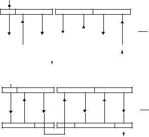
100 |
Steam Generators and Waste Heat Boilers: For Process and Plant Engineers |
Steam in
Gas in
|
|
|
|
|
|
|
|
|
|
|
|
|
|
|
|
|
|
|
|
|
|
|
|
|
|
|
|
|
|
|
|
|
|
|
|
|
|
|
|
|
|
|
|
|
|
|
|
|
|
|
|
|
|
|
|
|
|
|
|
|
|
|
|
|
|
|
|
|
|
|
|
|
|
|
|
|
|
|
|
|
|
|
|
|
|
|
|
|
|
|
|
|
|
|
|
|
|
|
|
|
|
|
|
|
|
|
|
(a) |
|
|
|
|
|
Steam out |
|
Steam in |
|
||||||||
|
|
|
|
|
|
||||||||||||
|
|
|
|
Steam in |
|
|
|
|
|
|
|
||||||
|
|
|
|
|
|
|
|
|
|
||||||||
Gas in
|
|
|
|
|
|
|
|
(b) |
Steam out |
||
FIGURE 3.15
Superheater arrangement for (a) low-pressure and (b) high-pressure operations.
what they have been doing for decades, many small boiler companies have found ways to offer better value to the end user if they modified the existing designs whenever necessary. In the following example, a standard boiler design for an application involving FGR was found to have a very high back pressure, though the initial cost was attractive. The back pressure was reduced by making a minor change to the convection bank as a result of which the operating cost of the boiler was significantly reduced. The boiler cost did not increase, while the fan size and power consumption were drastically reduced. A strong thermal engineering team is required in a boiler company to perform this type of analysis. Plant engineers should review the thermal performance and question the boiler suppliers regarding operating costs and back pressure. Since many boiler companies do not want to spend time reengineering their boiler and want to push existing designs, plant engineers will not get a satisfactory answer! However, by becoming more knowledgeable, they can easily see how a particular boiler design can be improved. The following example illustrates the point.
Example 3.1
A boiler supplier proposed a steam generator firing distillate oil with a capacity of 90,750 kg/h (200,000 lb/h) of saturated steam at 27.6 barg (400 psig) using 110°C (230°F) feed water to a chemical plant; to meet low emissions of NOx, the boiler supplier suggested the need for FGR at 17% and an excess air of 15%. On reviewing the boiler performance of the standard boiler, the plant engineer felt that the back pressure or flue gas pressure drop in the convection bank was high. The author also felt that the operating cost could be significantly reduced by making minor changes to the convection bank design without impacting the performance. The results are shown in Table 3.2 for the standard and custom designs showing how a small change can bring in so much relief in operating cost! The economizer exit gas temperature is the same in both cases,

Steam Generators |
101 |
TABLE 3.2
Comparison of Standard and Custom-Designed Boiler
Item |
Standard Boiler |
Custom Boiler |
|
|
|
Flue gas flow, kg/h |
110,940 |
110,950 |
Furnace exit temperature, °C |
1,130 |
1,130 |
Leaving evaporator, °C |
386 |
422 |
Leaving economizer, °C |
148 |
149 |
Evaporator surface, m2 |
552 |
552 |
Economizer surface, m2 |
2,370 |
2,495 |
|
Evaporator |
Economizer |
Evaporator |
Economizer |
Tubes/row |
12 |
20 |
12 |
20 |
Number of rows deep |
105 |
19 |
105 |
20 |
Tube length, m |
2.743 |
3.66 |
2.743 |
3.66 |
Transverse pitch, mm |
133 |
114 |
159 |
114 |
Gas press drop, mm wc |
286 |
33 |
150 |
36 |
Notes: Gas analysis: % volume CO2 = 11.57, H2O = 12.29, N2 = 73.63, O2 = 2.51. Fouling factor gas = 0.0006, and tube side = 0.0002 m2 h °C/kcal. Tube size = 50.8 × 44.7 mm. Fins configuration of economizer: 197 fins/m, 19 mm high, 1.27 mm thick, 4.36 mm serration.
and hence, the efficiency is the same. The boiler furnace and convection bank surface area remained the same. However, the evaporator tube spacing was manipulated in the custom boiler to lower the gas pressure drop. To compensate for the slightly higher gas temperature entering the economizer, one more row was added to the economizer. Hence, boiler cost did not see any increase! (A large company in my personal opinion may not be amenable to such design modifications as it involves several layers of bureaucracy to make these small changes or they may say that they have thousands of such standard boilers in operation worldwide, and if the plant engineers are not process-savvy, they may go along with the poor design losing money in operating costs year after year!)
The boiler practically is the same in both cases except for the tube spacing of the evaporator section and an additional row of tube in the economizer. However, the operating cost of the custom-designed boiler reduces by over 130 mm wc. The fan power saved is 2.7 × 10−6 × 90,000 × 130/(1.16 × 0.7) = 39 kW (1.16 kg/m3 is the density of air and 0.7 is the efficiency of fan motor combination and air flow = 90,000 kg/h). At 15 cents/kWh, the annual savings in operating cost due to this slight modification is = 39 × 0.15 × 8,000 = $46,800. Hence, the custom design pays for itself in a short period. It is not sufficient if the plant engineer reviews the painting or insulation or the welding aspects or weight of the boiler. The objective of the book is to make plant engineers process-savvy so that they can review boiler performance from boiler suppliers and suggest improvements or question their data!
Plant engineers can also verify the performance data for the standard and custom boilers as follows. Appendix A shows the procedure.
Solution
Calculations for Evaporator Performance in Standard Boiler
Gas mass velocity G = 110,940/[12 × 2.743 × (0.133 – 0.0508) = 41,000 kg/m2 h = 11.39 kg/m2s. Average gas temperature in the bank tubes = (1130 + 386)/2 = 758°C = 1031 K.
A good estimate of gas film temperature = 0.5 × (758 + 231) = 494°C or close to 500°C. Gas properties for heat transfer are evaluated at this temperature. From Appendix F,
102 |
Steam Generators and Waste Heat Boilers: For Process and Plant Engineers |
Cp = 0.2863 kcal/kg °C, µ = 0.1209 kg/m h, k = 0.046 kcal/m h °C. Tube wall temperature may be assumed to be 237°C, a little more than saturation due to the high tube-side boiling heat transfer coefficient of about 10,000 kcal/m2 h °C (assumed). As discussed in Appendix A, the tube-side coefficient will not impact U.
Let us use Grimson’s correlations for hc. For ST/d = 133/50.8 = 2.62 and SL/d = 101.6/50.8 = 2, from Table C.2, B = 0.213, N = 0.64.
Reynolds number Re = 41,000 × 0.0508/0.1209 = 17,227. Nu = 0.213 × 17,2270.64 = 109.5 = hc × 0.0508/0.046 or hc = 99.15 kcal/m2 h °C. A correction factor of 10% is used with Grimson’s correlations for convection bank with membrane panel end walls (based on the author’s experience). Hence, use hc = 109 kcal/m2 h °C.
Calculation of nonluminous heat transfer coefficient hn. Using methods discussed in Appendix D, beam length L = 1.08 × (0.133 × 0.1016 – 0.785 × 0.05058 × 0.0508)/0.0508 = 0.244 m. K = (0.8 + 0.12 × 1.6) × (1 − 0.00038 × 1031) × 0.238/(0.238 × .244)0.5 = 0.596.
g = 0.9 × [1-exp(.244 × 0.5960] = 0.122
hn = 5.67 × 10−8 × 0.122 × [10314 − 5104]/(1031 − 510) = 14.1 W/m2 K = 12.12 kcal/m2h°C (1031°K is the average gas temperature and 510 K is the average tube wall temperature.)
1/Uo = 1/(109 + 12.12) + 0.0006 + 0.0505 × ln(50.8/44.7)/(2 × 35) + 50.8/(44.7 × 9800) + 0.0002 × 50.8/44.7 or Uo = 107.6 kcal/m2 h °C (125.1 W/m2 K)
Let us check the evaporator exit gas temperature. One may use the following equation for evaporator performance as shown in Appendix A.
Ln[(1130−231)/(T – 231)] = 107.6 × 552/(110,941 × 0.303) or T = 385°C agrees with the data given by the boiler supplier (0.303 is the specific heat of flue gas at the average gas temperature).
Flue Gas Pressure Drop
MW of flue gas = 44 × 0.1157 + 18 × 0.1229 + 28 × 0.7363 + 32 × 0.0251 = 28.72. ST/d = 2.625.
SL/d = 2.
Density at average gas temperature of 758°C = 12.17 × 28.72/(273 + 758) = 0.339 kg/m3. Reynolds number at 758°C = 41,000 × 0.0508/0.1469 = 14,178. See Appendix C for flue
gas pressure drop calculations.
Friction factor f = 14,178−0.15[0.044 + 0.08×2/{1.625(0.43 + 1.13/2)}] = 0.034
P = 0.204fG2Nd/ρg = 0.204 × 11.392 × 0.034 × 105/0.339 = 279 mm wc, which is close to the boiler supplier’s data.
Calculations for Evaporator Performance in Custom Boiler
Now let us look at the option of ST = 159 mm. Average gas temperature is (1130 + 422)/2 = 776°C. G = 110,940/[12 × 2.743 × (0.159 – 0.0508) = 31,150 kg/m2 h = 8.65 kg/m2 s.
Approximate gas film temperature = 0.5 × (776 + 231) = 503°C, which is not much different from the earlier case. So let us use the same flue gas properties.
For ST/d = 3.125, SL/d = 2, B = 0.198, and N = 0.648 from Appendix C. Re = 31,150 × 0.0508/0.1209 = 13,088. Nu = 0.198 × 130,880.648 = 92.1 or hc = 92.1 × 0.046/0.0508 = 84.3 kcal/m2 h °C. Using 10% margin as before, hc = 91.8 kcal/m2 h °C.
Beam length L = 1.08 × (0.159 × 0.1016 – 0.785 × 0.05058 × 0.0508)/0.0508 = 0.300 m
K = (0.8 + 0.12 × 1.6) × (1−0.00038 × 1049) × 0.238/(0.238×.300)0.5 = 0.531
g = 0.9 × [1 – exp(–.0300x0.531] = 0.132

Steam Generators |
103 |
hn = 5.67 × 10−8 × 0.132 × [10494−5104]/(1049−510) = 15.87 W/m2 K = 13.65 kcal/m2 h °C
1/Uo = 1/(91.8 + 13.65) + 0.0006 + 0.0505 × ln(50.8/44.7)/(2 × 35) + 50.8/(44.7 × 9800) + 0.0002 × 50.8/44.7 or Uo = 95 kcal/m2 h °C (110.5 W/m2 K).
Let us compute the exit gas temperature T. Ln[(1130 − 231)/(T – 231)] = 95 × 552/(110,941 × 0.303) or T = 420°C agrees with the data given by the boiler supplier.
Flue Gas Pressure Drop
Reynolds number at average gas temperature of 776°C = 31,150 × 0.0508/0.1486 = 10,649. Friction factor f = 10,649−0.15[0.044 + 0.08 × 2/{2.125(0.43 + 1.13/2)}] = 0.0297.
P = 0.204fG2Nd/ρg = 0.204 × 8.652 × 0.0297 × 105/0.333 = 143 mm wc, which is close to the value shown. Density of flue gas at average gas temperature is 0.333 kg/m3.
Economizer Performance
A simple way of checking the economizer duty will be explained as the economizer design or cross section is unchanged. Calculate the LMTDs for both cases and the duty that is proportional to the temperature rise of the water. The ratio of the duty for custom to standard economizer is Qc/Qs = (Uc × Tc × 2495)/(Us × Ts × 2370) = 87/76 (87°C and 76°C refer to water temperature rise, which is a proxy for the duty as water flow is the same in both cases and the surface areas are, respectively, 2495 and 2370 m2).
Tc = [(386 − 186) – (148 − 110)]/ln[(386 − 186)/(148 − 110)] = 97.5°C.
Ts = [(422 − 197) – (149 − 110)]/ln[(422 − 197)/(149 − 110)] = 106°C
Hence, (Uc × 106 × 2495)/(Us × 97.5 × 2370) = 87/76 or Uc/Us > 1. That is, it is sufficient if Uc is equal to Us to transfer the desired duty in the economizer. However, note that Uc will be higher than Us as the average gas temperature in the economizer is now higher. Hence, the duty Qc can be easily achieved. Hence, the custom design is a far better offering than the initial standard design. Only by challenging the boiler supplier, a better design emerged. Thus, plant engineers should have process-oriented background, and this book will help them become a little more process-savvy.
Boiler Classification
Boilers may be classified into several categories depending on the following:
1.By application as utility, marine, or industrial boiler. Utility boilers are the large steam generators used in power plants generating 500–1000 MW of electricity. They are generally fired with solid fuels, pulverized coal, or fluidized bed furnaces. Utility boilers generate high-pressure, high-temperature superheated and reheated steam; typical steam parameters are 16,500 kPa (165 barg), 540°C/540°C. A few utility boilers generate supercritical steam at 240 barg, 590°C/590°C/590°C with double reheat systems. Industrial boilers used in cogeneration plants generate steam at varying steam pressures of 10–100 barg at steam temperatures ranging
104 |
Steam Generators and Waste Heat Boilers: For Process and Plant Engineers |
from saturation to 500°C. They are generally fired on oil and gas. Industrial boilers may import saturated steam from other boilers to be superheated or export saturated steam with the balance being superheated. Hence, their designs are more challenging.
2. By circulation methods: Figure 2.6 illustrates the concepts of natural, forced, or controlled and once-through steam generators (OTSGs). Natural circulation designs are used up to 165 barg steam pressure. Beyond this, a controlled circulation system using circulating pumps is preferred. A small operating cost is involved for moving the steam water mixture through the evaporator tubes. However, the circulation ratio (CR) may be kept small based on the design and experience of the boiler supplier. CR of 4–7 is common. The once-through design concept may be implemented at any pressure of steam. However it requires zero solids feed water; else deposits inside tubes while evaporation occurs would increase the evaporator tube wall temperature and damage the tubes particularly in the high heat flux region.
3. By fuel type: Type of fuel-fired influences the boiler size significantly. Solid fuel requires low heat release rates as combustion is difficult, and more residence time is required in the furnace. Oiland gas-fired furnaces can be smaller. The furnace absorption with oil firing is more due to the higher intensity of flame radiation, and hence, the furnace for oil fuels is slightly larger. This is discussed in Chapter 2.
Steam pressure also affects the boiler furnace size. As can be seen from Chapter 2, the latent heat of steam is much higher at lower steam pressure compared to higher steam pressure. The liquid heat or the energy pickup from feed water temperature at economizer inlet to the saturated steam point is much higher as the steam pressure increases. Hence, very high-pressure boilers may have a small furnace and no evaporator or boiler bank to speak of and a large superheater and a large economizer, while a low steam pressure boiler will have a large furnace and a boiler bank or evaporator and a small superheater and a small economizer.
4.Type of boiler: package boilers are classified as A, D, or O type depending on their construction as shown in Figures 3.16 and 3.17.
O-type boilers: This boiler has a steam drum and a bottom drum and has a cross section like the letter O. It is symmetrical in design and hence can be shipped easily, which is why this type of design is favored in rental boiler industry where a boiler may be used at various locations during its lifetime. The gas outlet is at the burner end and at the top. An economizer may be located in the gas outlet duct. If a convective superheater is required, it has to be split up as shown in the A-type boiler. If two-stage superheater with interstage attemperation is required, it adds to the complexity of piping, and two desuperheaters are required. A radiant superheater as shown in Figure 3.16a may be used, but unless the furnace is properly sized, flame can impinge on the superheater tubes, causing it to sag or even overheat and fail.
The A type is similar in features to the O-type boiler and being symmetrical in construction is well suited for frequent movements as a rental boiler. The convective superheater has to be split and located in the two parallel sections of the convection bank, while the radiant superheater is similar to that used in the O type. Using a single-stage radiant section is not advisable as temperature control is difficult. Hence, a combination of convection and radiant superheaters is preferred. This is discussed later.
The D type is well suited for large boiler capacities with high controlled steam temperatures (Figures 3.16d and 3.17a, b). Since all the flue gas goes through the convection bank, there is no question of maldistribution between the two convection passes as in A- or O-type boilers.

Steam Generators |
105 |
When steam temperature control is required, it is desirable to use a screen section followed by a two-stage superheater with a desuperheater in between. The economizer can be located in the horizontal gas flow direction as shown in Figure 3.17a to make the arrangement simple. More space is required for the D-type boiler as the gas exit is at the side and not at the boiler front as in O- and A-type boilers. Figure 3.17b shows the economizer of a D-type boiler in the vertical gas flow direction. The stack can be mounted on top of the economizer.
(a)
(b)
FIGURE 3.16
(a) A-type boiler, (b) O-type boiler,
(Continued)

106 |
Steam Generators and Waste Heat Boilers: For Process and Plant Engineers |
(c)
(d)
FIGURE 3.16 (Continued)
(c) A-type boiler with superheater, and (d) D-type boiler with superheater. (Courtesy of Cleaver Brooks Inc., Engineered Boiler Systems, Thomasville, GA.)
Steam Generators |
107 |
||||||||||||||||||||||||||||||||
|
|
|
|
|
|
|
|
|
|
|
|
|
|
|
|
|
|
|
|
|
|
|
|
|
|
|
|
|
|
|
|
|
|
|
|
|
|
|
|
|
|
|
|
|
|
|
|
|
|
|
|
|
|
|
|
|
|
|
|
|
|
|
|
|
|
|
|
|
|
|
|
|
|
|
|
|
|
|
|
|
|
|
|
|
|
|
|
|
|
|
|
|
|
|
|
|
|
|
|
|
|
|
|
|
|
|
|
|
|
|
|
|
|
|
|
|
|
|
|
|
|
|
|
|
|
|
|
|
|
|
|
|
|
|
|
|
|
|
|
|
|
|
|
|
|
|
|
|
|
|
|
|
|
|
|
|
|
|
|
|
|
|
|
|
|
|
|
|
|
|
|
|
|
|
|
|
|
|
|
|
|
|
|
|
|
|
|
|
|
|
|
|
|
|
|
|
|
|
|
|
|
|
|
|
|
|
|
|
|
|
|
|
|
|
|
|
|
|
|
|
|
|
|
|
|
|
|
|
|
|
|
|
|
|
|
|
|
|
|
|
|
|
|
|
|
|
|
|
|
|
|
|
|
|
|
|
|
|
|
|
|
|
|
|
|
|
|
|
|
|
|
|
|
|
|
|
|
|
|
|
|
|
|
|
|
|
|
|
|
|
|
|
|
|
|
|
|
|
|
|
|
|
|
|
|
|
|
|
|
|
|
|
|
|
|
|
|
|
|
|
|
|
|
|
|
|
|
|
|
|
|
|
|
|
|
|
|
|
|
|
|
|
|
|
|
|
|
|
|
|
|
|
|
|
|
|
|
|
|
|
|
|
|
|
|
|
|
|
|
|
|
|
|
|
|
|
|
|
|
|
|
|
|
|
|
|
|
|
|
|
|
|
|
|
|
|
|
|
|
|
|
|
|
|
|
|
|
|
|
|
|
|
|
|
|
|
|
|
|
|
|
|
|
|
|
|
|
|
|
|
|
|
|
|
|
|
|
|
|
|
|
|
|
|
|
|
|
|
|
|
|
|
|
|
|
|
|
|
|
|
|
|
|
|
|
|
|
|
|
|
|
|
|
|
|
|
|
|
|
|
|
|
|
|
|
|
|
|
|
|
|
|
|
|
|
|
|
|
|
|
|
|
|
|
|
|
|
|
|
(a)
(b)
FIGURE 3.17
(a) D-type boiler with horizontal gas flow economizer and (b) D-type boiler with economizer in vertical gas flow direction. (Courtesy of Cleaver Brooks Inc., Engineered Boiler Systems, Thomasville, GA.)
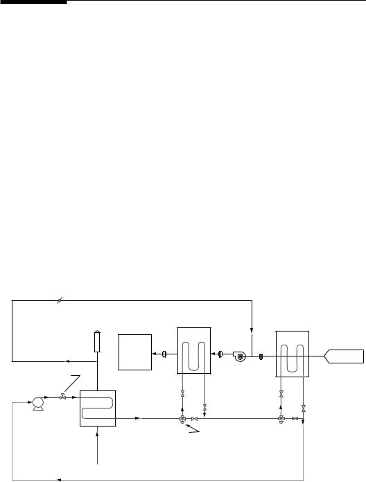
108 |
Steam Generators and Waste Heat Boilers: For Process and Plant Engineers |
Improving Boiler Efficiency
Typical efficiency on lower heating value (LHV) basis for a natural gas–fired boiler is about 93% with 150°C exit gas temperature. In the boiler with elevated steam drum (Figure 3.3), a novel glycol-based closed-loop heat recovery system was incorporated to improve the boiler efficiency by about 2.5% with the exit gas temperature controlled at about 101°C, lower than the feed water temperature! The system also helps increase the air temperature to the forced draft in severe Canadian winter conditions when ambient air temperature ranges from –10°C to –40°C! The scheme is shown in Figure 3.18. There are three glycol heat exchangers in this concept. The boiler capacity is 193 t/h of steam at 3800 kPa with110°C feed water temperature. The package boiler assembly consists of the furnace and convection bank as a single unit built in the shop and was the largest that could be shipped by land in the United States and Canada. Headers were used for the convection bank instead of steam and mud drums. The steam drum was connected to the boiler bank by a system of external downcomers and riser piping. This approach enabled the large steam drum to be shipped separately. Furnace projected area and volume were also liberally sized so that the furnace heat release rates on volumetric and area basis are low, 587,000 kcal/m3 h (66,000 Btu/ft3 h) and 481,000 kcal/m2 h (177,000 Btu/ft2 h). The drum holdup time also was large exceeding 5.5 min from normal level to empty as there was no shipping limitation for the drum.
The boiler efficiency was shown to be 86% on HHV basis while generating 193 t/h of steam. The closed-loop glycol system has two air heaters that can be bypassed on glycol side. The first finned tube air heater preheats cold ambient air entering the fan and maintains it at a minimum temperature of about 10°C after mixing with the recirculated flue gas.
Flue gas recirculation
|
Air heater #2 |
To stack |
|
Flue gas temperature |
|
maintained at 100°C |
Natcom |
|
burner |
FD Fan
Glycol flow managed based on boiler load
Air heater #1
Amient air 40°C–27°C
Scavenger
Glycol
pump
Glycol flow through airheater #2 controlled to optimize heat recovery
Glycol flow through air  heater #1 controlled to maintain
the air temperature
at fan inlet between 5°C and 40°C
Economizer |
60% glycol water mixture |
gas outlet |
FIGURE 3.18
Scheme for improving boiler efficiency using glycol heat recovery system. (Courtesy of Cleaver Brooks Inc., Engineered Boiler Systems, Thomasville, GA.)

Steam Generators |
|
109 |
||
|
TABLE 3.3 |
|
|
|
|
Field Data for the Elevated Drum Boiler |
|
|
|
|
|
|
|
|
|
Parameter |
100% Load |
120% Load |
|
|
|
|
|
|
|
Steam flow, t/h |
160 |
192 |
|
|
Steam pressure, kPa |
3751 |
3751 |
|
|
Feed water in |
110 |
110 |
|
|
Oxygen in flue gas,% |
2.3 |
2.2 |
|
|
NOx ppmv |
46 |
44 |
|
|
Flue gas recirculation, % |
10 |
11 |
|
|
Ambient temperature, °C |
21 |
22 |
|
|
At air heater exit, °C |
66 |
82 |
|
|
Exit gas temperature, °C |
103 |
108 |
|
Note: Typical exit gas temperature would have been 150°C–160°C.
The second air heater, located after the fan, preheats the mixture of flue gas recirculated for NOx control and air from the fan. This glycol bypass system maintains the stack gas temperature at about 101°C. If the ambient air temperature is high, as it is in summer, then either air heater may be shut off and the glycol flow bypassed on the tube side of either air heater, as very hot combustion air will increase NOx production. The as-tested performance of the plant is summarized in Table 3.3 [2,3].
Figure 3.19 shows a scheme for improving the efficiency of a gas-fired boiler without using any thermic fluid heating system as discussed earlier. Incoming air from the forced draft fan is heated to about 65°C–75°C by a portion of the feed water. (In case there is no NOx concern, the air temperature can be even further increased and the exit gas temperature from the economizer can be lowered further.) The cooled feed water is heated in another exchanger called scavenger located behind the regular economizer. The increase in air temperature is approximately equal to the drop in flue gas temperature beyond the economizer. If there are no NOx or acid dew point concerns, then the flue gas can be cooled to a lower temperature. This scheme does not require a heat sink such as makeup water to lower the flue gas temperature from the system. Efficiency improvement can be in the range of 1.5%–2% over conventional plants, and the additional cost of the two finned coils and air/gas pressure drop will pay for itself in a short period depending on local fuel cost and the cost of electricity. (This scheme is being patented by Cleaver Brooks, Nebraska, boiler division.)
Adding Condensate Heater to Improve Boiler Plant Efficiency
As in HRSGs, one may consider adding a condensate heater in case the makeup water flow is high enough as shown in Figure 3.20. A heat exchanger may also be used to lower the feed water temperature and preheat the makeup in a separate heat exchanger or a condensate heater may be used as shown. One should use appropriate materials when water inlet temperature to condensate heater drops below the water dew point as discussed in Chapters 1 and 6. Another option is shown in Figure 3.20a, where a heat exchanger is used to lower the feed water temperature to the economizer thus preheating the makeup water, which enables reduction in deaeration steam.

110 |
Steam Generators and Waste Heat Boilers: For Process and Plant Engineers |
To DA |
Min. Recirc. |
|
From DA
Feed pump
Fresh air |
FD fan |
|
|
30–100°F |
|
% MCR |
To stack |
Firing rate |
220–230°F |
|
|
|
TG0 |
|
45,000 LB/HR at ~150°F |
|
|
|
|
|
Scavenger |
TW1 |
~255°F |
Flow control station |
TG1 300°F |
|
|||
|
|
Feedwater |
Economizer |
|
202,000 LB/HR at ~250°F |
||
|
FE1 |
|
|
|
|
Drum |
|
|
|
|
760°F |
Burner
160–170°F
200,000 LB/HR,  900 PSIG, 865°F
FIGURE 3.19
Scheme to improve boiler efficiency. (Patented by Cleaver Brooks Inc., Engineered Boiler Systems, Thomasville, GA.)
1 |
|
4 |
1 |
7 |
4 |
7 |
|
||||
|
|
||||
|
|
|
|
2 |
|
|
|
|
|
|
|
|
|
|
2 |
|
5 |
|
|
|
|
|
|
|
|
|
5 |
|
|
|
|
8 |
|
|
|
|
3 |
|
|
3 |
9 |
|
|
|
|
|
|
Heat exchanger |
|
Condensate heater |
|
||
|
|
|
|
||
FIGURE 3.20
Scheme to increase boiler plant efficiency using a heat exchanger and lower feed water temperature to economizer. Note: (1) turbine, (2) deaerator, (3) HRSG, (4) mixing tank, (5) pump, (6) deaerator coil, (7) condenser,
(8) heat exchanger, (9) condensate heater.

Steam Generators |
111 |
TABLE 3.4
Effect of Lower Feed Water Temperature
Item |
Case 1 |
Case 2 |
|
|
|
Steam flow, kg/h |
90,740 |
90,740 |
Steam pressure, barg |
27.6 |
27.6 |
Feed water temp., °C |
110 |
60 |
Blowdown,% |
1 |
1 |
Exit gas temp., ±°C |
153 |
115 |
Efficiency, % LHV |
93.2 |
95.0 |
Efficiency, % HHV |
84.1 |
85.74 |
Energy to steam, MM kcal/h |
50.78 |
55.37 |
Fuel LHV, MM kcal/h |
54.48 |
58.28 |
|
|
|
Example 3.2
A 90,740 kg/h (200,000 lb/h) natural gas–fired D-type package boiler is generating saturated steam at 27.6 barg (400 psig) with feed water at 110°C (230°F) in a cogeneration plant. Customer is using a lot of steam in the deaerator and wants to know if the feed water can be used to preheat the makeup water–condensate mixture entering the deaerator and thus lower the deaeration steam requirements and whether this scheme has any benefit to him. Customer thinks he can cool the feed water to 60°C and the makeup water mixture can enter the deaerator much hotter and thus save his energy requirements. With 60°C feed water, there is no concern about water dew point condensation as natural gas is fired in the boiler with partial pressure of water vapor about 0.18. Water dew point corresponds to 57°C from steam tables.
The boiler performance was simulated with feed water at 110°C and at 60°C. Results are shown in Table 3.4. Note that the boiler size has not changed in these options—only the feed water temperature.
The scheme may be evaluated in a few different ways. If deaeration steam is taken from the boiler itself, then one can increase the boiler steam capacity based on deaeration steam requirement for each case and see the difference. But it is obvious that even though the fuel-fired is 3.8 MM kcal/h more, the additional energy recovered in the entire system due to the higher condensate temperature entering the deaerator will be 90,740 × 1.01 ×(110−60) = 4.58 MM kcal/h. Hence, the scheme is more efficient; one has to consider the additional cost of the heat exchanger and associated piping valves for cooling the feed water, but it is worth considering if an appropriate heat sink is available.
Understanding Boiler Performance
It is important for plant engineers to have an idea of how the various important parameters such as efficiency, exit gas temperature, and water temperature beyond the economizer vary with load. Many refineries have both steam generators and fired HRSGs. Knowing this trend in performance versus load for both the steam generator and HRSG, one can load each of the equipment such that the maximum steam is generated at the lowest fuel consumption. This is discussed in Chapter 4. Presented in Figure 3.21 is the performance chart of a gas-fired steam generator showing how the various parameters vary with load. It may be seen as follows:
1.The efficiency curve shows a parabolic trend. This is due to the combination of casing loss, that increases as the load decreases and the other heat losses that decrease as the load decreases. This trend is also explained in Chapter 1.

112 |
Steam Generators and Waste Heat Boilers: For Process and Plant Engineers |
|
420 |
|
|
|
|
|
Steam temperature |
|
||
|
370 |
|
|
|
|
|
|
|||
|
|
|
|
|
|
E•ciency |
|
|
|
|
°C |
|
|
|
|
|
|
|
|
|
|
320 |
|
|
|
|
|
|
|
|
|
|
Temperature, |
220 |
|
|
|
|
|
Water leaving econ. |
|
||
|
270 |
|
|
|
|
|
|
|
|
|
|
170 |
|
|
|
|
|
Exit gas temperature |
|
||
|
|
|
|
|
|
|
|
|||
|
12020 |
30 |
40 |
50 |
60 |
70 |
80 |
90 |
100 |
|
|
|
|
|
|
|
Load, % |
|
|
|
|
FIGURE 3.21
Steam generator performance versus load.
95
94
93
92 %
91 |
efficiency, |
|
|
90 |
|
89 |
LHV |
88 |
|
87 |
|
86 |
|
85 |
|
2.The exit gas temperature and water temperature leaving the economizer increase as the load increases. This is due to the higher mass flow of flue gases at higher gas temperatures as the load increases. Unlike the HRSG, steaming is rare in steam generator economizer as the ratio between air flow and steam flow is maintained by combustion control system. If the economizer is sized so that it does not steam at full load, it will never steam at part loads. The approach point (difference between the saturation temperature and water temperature leaving the economizer) keeps increasing as the load decreases, while it shows the opposite trend in gas turbine HRSGs.
3.The steam temperature increases as the load increases if a convective-type superheater is used. This type of superheater is generally suggested up to about 500°C. For higher steam temperatures, one may consider a combination of radiant and convective superheaters. The features of radiant and convective superheaters are discussed later. The furnace exit gas temperature is lower on oil fuel firing compared to natural gas. Hence, the superheater is sized based on oil firing. With natural gas firing, the gas temperature at the superheater increases, which can be controlled using spray desuperheater.
4.The feed water temperature leaving the economizer is higher at higher loads in a steam generator, while it is lower at higher loads in an HRSG. Hence, we have the steaming problem in economizer with HRSGs, while it is absent in steam generators.
Why Economizer Does Not Steam in Steam Generators
In a steam generator, the ratio between the fuel flow and steam flow is maintained at all loads through combustion control; this results in a flue gas flow to steam ratio of about 1.1 at normal loads and about 1.3–1.5 at lower loads. However, in a gas turbine HRSG, the exhaust gas mass flow remains somewhat constant at all loads, while the steam flow varies with exhaust gas inlet temperature. The ratio between exhaust gas and steam can be as high as 7–10 at low loads. At low loads, the HRSG makes lesser steam due to the lower exhaust gas inlet temperature. Since the economizer water flow matches the steam flow, the combination of low water flow through the economizer with large exhaust gas flow

Steam Generators |
113 |
results in relatively large energy transfer in the economizer and high enthalpy pickup in the feed water causing it to generate steam or reach temperatures close to saturation. On the other hand, at part loads, the flue gas temperature to the economizer drops off in a steam generator along with flue gas flow. Hence, the water temperature leaving the economizer is lower at lower loads and the steaming issue does not arise in steam generators. The approach point (difference between saturation temperature and water temperature leaving the economizer) increases as load decreases, while in an HRSG, it is the other way. This point is also elaborated in Chapter 5 on HRSG simulation.
Understanding Boiler Surface Areas
Many plant engineers and purchase managers make the mistake of evaluating or purchasing boilers solely based on surface areas. The misconception is that more surface area, better the boiler and more steel is offered! This is a wrong notion. In HRSGs, for example, we can show that based on fin geometry, one can have 50%–100% more surface area and yet have the same performance!! In steam generators, 15% difference in surface areas is not uncommon based on furnace sizing, location, and type of superheater whether convective or radiant and fin geometry used for the economizer.
Example 3.3
For a 60 t/h, 28 kg/cm2g, 400°C gas-fired steam generator with feed water at 110°C, two boiler designs are being offered, one with a semi-radiant superheater and another with convective superheater. The tube geometry details of both designs are shown in Tables 3.5 and 3.6. (Incidentally, any steam generator or HRSG supplier should provide data for his boiler in this format.) Tube material information may also be included for each section. If there are more heating surfaces, each of them should have the data shown. Streams are the number of tubes that carry the total flow; this has been explained in Appendix B.
TABLE 3.5
Geometric Data with Convective Superheater
Geometry |
Screen |
Sh1 |
Evap. |
Econ. |
|
|
|
|
|
Tube OD, mm |
50.8 |
50.8 |
50.8 |
50.8 |
Tube ID, mm |
44.7 |
44 |
44.7 |
44.7 |
Fins/m |
0.000 |
0.000 |
0.000 |
197 |
Fin height, mm |
0.000 |
0.000 |
0.000 |
19 |
Fin thk., mm |
0.000 |
0.000 |
0.000 |
1.25 |
Fin width, mm |
0.000 |
0.000 |
0.000 |
4 |
Fin conductivity |
0.000 |
0.000 |
0.000 |
37 |
Tubes/row |
12 |
12 |
12 |
16 |
Number of rows deep |
11 |
24 |
60 |
9 |
Length, m |
2.750 |
2.7 |
2.75 |
4.8 |
Tr pitch, mm |
137 |
137 |
137 |
101 |
Long pitch, mm |
101 |
125 |
101 |
101 |
Streams |
0.000 |
24.000 |
0.000 |
8.000 |
Parl = 0, countr = 1 |
0.000 |
1.000 |
0.000 |
1.000 |
Note: Furnace length = 10.67 m, width = 2.14 m, height = 2.05 m.

114 |
Steam Generators and Waste Heat Boilers: For Process and Plant Engineers |
TABLE 3.6
Geometric Data with Radiant Superheater
Geometry |
Screen |
Sh1 |
Evap. |
Econ. |
|
|
|
|
|
Tube OD, mm |
50.8 |
50.8 |
50.8 |
50.8 |
Tube ID, mm |
44.7 |
44 |
44.7 |
44.7 |
Fins/m |
0.000 |
0.000 |
0.000 |
197 |
Fin height, mm |
0.000 |
0.000 |
0.000 |
19 |
Fin thk., mm |
0.000 |
0.000 |
0.000 |
1.25 |
Fin width, mm |
0.000 |
0.000 |
0.000 |
4 |
Fin conductivity |
0.000 |
0.000 |
0.000 |
37 |
Tubes/row |
12 |
12 |
12 |
16 |
Number of rows deep |
2 |
16 |
67 |
12 |
Length, m |
2.750 |
2.7 |
2.75 |
4.8 |
Tr pitch, mm |
137 |
137 |
137 |
101 |
Long pitch, mm |
101 |
125 |
101 |
101 |
Streams |
0.000 |
24.000 |
0.000 |
8.000 |
Parl = 0, countr = 1 |
0.000 |
1.000 |
0.000 |
1.000 |
Note: Furnace length = 9.14 m, width = 1.83 m, height = 2.05 m.
One may see that the overall performance is nearly the same with both the options. The total surface area of the radiant superheater design is about 12% lesser compared to the convective superheater option. The fan power consumption is the same as the back pressure. Efficiency also is close. The heat release rates are reasonable, and though the heat flux with the smaller furnace is more, it is far below the allowable limits for departure from nucleate boiling (DNB) and hence acceptable. The radiant superheater has a higher tube wall temperature, but considering the low steam pressure, the thickness provided is adequate. Life of the radiant superheater may be shorter if we use the Larsen Miller chart for life estimation, but it is likely to exceed the expected 40 years at these temperatures. One has to check the part load performance to see if this is acceptable and make a decision. The convective superheater design, even though it may be more expensive, is preferred for the comfort factor it offers and its longer life. However, the purpose
TABLE 3.7
Summary of Performance for Radiant and Convective Superheaters
Item |
Radiant SH |
Convective SH |
|
|
|
Volumetric heat release rate, kcal/m3 h |
928,500 |
680,560 |
Area heat release rate, kcal/m2 h |
482,400 |
389,352 |
Exit gas temperature, °C |
167 |
164 |
Flue gas flow, kg/h |
75,618 |
75,430 |
Efficiency, % LHV |
92.5 |
92.7 |
Back pressure, mm wc |
236 |
227 |
Furnace projected area, m2 |
98 |
122 |
Superheater surface, m2 |
64 |
97 |
Evaporator, m2 |
399 |
410 |
Economizer, m2 |
1,036 |
1,221 |
Economizer fin geometry |
118 × 19 × 1.26 × 4 |
197 × 19 × 1.26 × 4 |
Furnace width × length × height, m |
1.83 × 9.14 × 2.05 |
2.14 × 10.67 × 2.05 |
Type of superheater |
Radiant |
Convective |
Superheater tube temperature, °C |
560 |
510 |
|
|
|

Steam Generators |
115 |
of the exercise is to show that variations in surface areas can be there for the same overall performance, and operating cost and the design with lesser surface area cannot be ignored but properly evaluated (Table 3.7).
Steam Generators for Oil Sands Application
Steam-assisted gravity drainage (SAGD) is considered to be the most viable and environmentally safe recovery technology for extracting heavy oil and bitumen. In the SAGD process, one well is drilled above the bitumen deposit and a second one below the deposit. The upper well is supplied with high-pressure steam, and the lower well collects the heated oil or bitumen that flows out along with any water from the condensation of injected steam. The bitumen and water are pumped out, and they travel to a tank where the two elements are separated. The produced water is then cleaned, and it returns to the boiler where it is converted to steam and reinjected into the well. In the past, warm lime softening process was used to clean the oil field produced water. The produced water cannot be cleaned enough for conventional drum-type boilers so steam is generated in OTSGs making 75–80% quality steam, and hence, 20% of the water is wasted. Environmental regulations are becoming stricter in Alberta causing oil companies to focus on water conservation. As a result, a more viable and environmentally friendly technology called evaporator technology is replacing the warm line softening treatment process.
Evaporator technology produces higher-quality water compared to warm lime softening. The process takes the clarified water and evaporates it out and then condenses it back to produce feed water. It also conserves water and opens up the steam production options to drum-type boilers generating saturated steam. Evaporator water can be run through an OTSG or drum-type boiler (for medium pressure) or through Cleaver Brooks’s newly developed forced circulation oil sands steam generator (FC-OSSG). The special design feature of the FC-OSSG is that it operates like an OTSG but can be mechanically cleaned or pigged by conventional means.
The FC-OSSG addresses the key requirements of oil industry professionals:
•Ability to handle the inevitable water quality upsets
•Capability of operating with evaporator-produced water while delivering best- in-class efficiency
•Ability to handle capacities up to 227 t/h of steam (500,000 lb/h)
•Meeting stringent regulatory requirements for water usage and emissions
•Features reliable steam generators that can work with available produced water
•Easy to maintain—all circuits are piggable (a metal piece is sent through each circuit to clean the inside surface, which is called a pig and the process is called pigging)
Figure 3.4 shows the steam generator for oil sands applications. Figure 3.22 shows the scheme of the forced circulation boiler. There are two parallel circuits, one for the furnace section and another for the convective evaporator section. The circulation system is designed for an average CR of about 5. By varying the flow through the radiant or convective section, one can adjust the CR in either path. The tube wall temperatures in the furnace and evaporator section are measured, which gives an indication of any tube-side buildup of solids. The CR can be increased in that circuit if need arises.
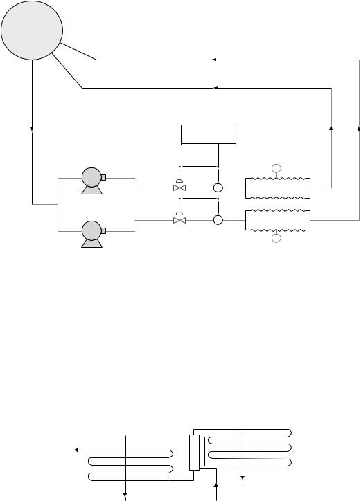
116 |
Steam Generators and Waste Heat Boilers: For Process and Plant Engineers |
Steam drum
20% quality
20% quality
Flow > 5 × steam ow
Flow rate decided by •ring rate
water quality
FE
2 × 50%
circulation pumps
FE
TE 12 o tube metal temperature
28 parallel passes Convection module
12 parallel passes Furnace module
TE 12 o tube metal temperature
FIGURE 3.22
Scheme of forced circulation boiler (FC-OSSG) for oil field application. (Courtesy of Cleaver Brooks Inc., Engineered Boiler Systems, Thomasville, GA.)
The issue of water quality upsets is one that is important to oil industry professionals. Existing technologies repeatedly fall short in this area. Even though a system may be operating with evaporated water, which is supposed to be pure, it may still contain oil content above the acceptable limit for drum boilers. This, along with the inevitable water quality upsets, can cause fouling of the heat transfer tubes. Cleaning drum boilers requires access to the inside drums, which are not piggable, so tube cleaning can be costly and time-con- suming. Alternatively, the OTSG can handle water quality upsets, but the equipment is limited in size. An OTSG can handle only up to 136 t/h (300,000 lb/h) of steam (Figure 3.23).
Turbine exhaust in |
Economizer |
|
80% steam out |
Heat exchanger |
|
|
|
|
70 F water in
Evaporator
FIGURE 3.23
OTSG generating 80% quality steam in oil fields.
Steam Generators |
117 |
Temperature
Subcooled water |
Two-phase, steam water |
Superheated steam |
|||||||||
|
|
|
|
High |
|
|
|
||||
|
|
|
heat ux |
|
|||||||
|
CHF |
|
|
|
|
|
Moderate |
Tube wall |
|||
|
|
|
|
|
|
|
|
heat ux |
|
|
|
|
|
|
|
|
|
|
|
|
|
|
temperatures |
|
|
Fluid temperature |
|
||||||||
Tube wall temperatures |
|
|
|
|
|
|
|
|
|
|
|
Water enthalpy |
|
|
|
|
|
|
|
|
|
|
Steam enthalpy |
|
0 |
|
|
|
|
|
|
|
|
|
100 |
|
x = Quality, % steam by weight |
|
|||||||||
FIGURE 3.24
Typical steam quality versus tube wall temperature in boiling process.
The FC-OSSG is a forced circulation boiler (Figure 3.4). It uses circulation pumps to force the steam water mixture through the furnace and evaporator circuits. A CR of 5–8 is achieved depending on the actual resistance to flow in the circuits. Hence, the steam quality at the exit of the furnace or evaporator is about 12%–20% only compared to 80% for an OTSG. Hence, allowable heat fluxes for DNB are much higher as shown in Figure 3.24 and as also discussed in Chapter 2. Higher fouling compared to OTSG can be handled by OSSG. The tube-side velocities are designed to be very high (on the order of 2.5 m/s). Hence, deposition of solids is ruled out, and frequency of cleaning and potential for failure will be less compared to an OTSG.
In case of upsets or sudden increase in feed water conductivity and turbidity over limits set, the control system reduces the firing rate on the boiler and increases the water flow through the tube to protect it. Increasing the amount of water flowing through the tube reduces the steam quality in the heat transfer circuits, resulting in lesser concentration of impurities and reduced metal temperatures. Heat flux also is reduced due to lowering of heat input. The boiler keeps running, but at a reduced firing rate. Then, if it exceeds another preset value, the operator trips the boiler to protect it.
Unlike in an OTSG, whereby mostly steam travels through the tube, the FC-OSSG is designed so that mostly water flows through the tube. The metal temperature of a waterfilled tube closely matches the water temperature rather than the hot gas temperature. For a constant heat flux (rate at which heat is transferred), the tube wall temperature is a function of the steam quality. At lower steam qualities, the tube predominantly is filled with water, and the metal temperature is closer to the water temperature and is stable. As the steam quality increases, the metal temperature also increases, and beyond a certain point, it starts dropping down, due to the very high velocities in the tube caused by the difference in densities of steam and water. Figure 3.24 shows the relationship between steam quality and metal temperature.

118 |
Steam Generators and Waste Heat Boilers: For Process and Plant Engineers |
An OTSG operates at 75%–80% steam quality, to the right of the curve, in the high steam quality region. Trying to predict the metal temperature in this region is very difficult. Conversely, the FC-OSSG operates at 20% steam quality, represented by the flat part of the curve, in the very robust, reliable operating region. Thus, it has much higher tolerance for any heat flux and water quality variations during operation. Several such steam generators are in operation today in Canada, supplied by Cleaver Brooks Corporation.
Superheaters
The superheater is an important component of a package boiler. Steam temperature can vary from saturation temperature to 500°C depending on the steam pressure and application. Steam pressure in industrial boilers can vary from 1000 kPa (10 barg) to 103 barg. In natural circulation utility boilers, steam pressure can be as high as 165 barg (2400 psig) with superheater and reheater steam temperatures at 540°C (1005°F).
Superheaters can be located in radiant or convection zone depending on application, boiler configuration, and steam temperature required. In a package boiler, a radiant superheater receives direct radiation from the flame in the furnace, while convective superheater is shielded by several rows of screen tubes as shown in Figure 3.25. A convective superheater with horizontal tubes is shown in Figure 3.26a and b, while in Figure 3.27, an inverted-loop superheater is shown with vertical tubes. Note that the tube lengths vary between the headers. The tubes in the middle of the convection bank are the shortest and hence will have more steam flow compared to the longer tubes at the ends. However, one should also note that the maximum heat transfer occurs in the middle of the section and tapers off at the ends. Hence, a self-compensating effect is provided by this design, and this design is used in almost all package boilers. The horizontal tube design has the same length of tubes in all streams, and hence, the nonuniformity in steam flow is minimal. The shorter tube length and more sections may increase the cost of manufacturing, but both designs are used in the industry. Superheaters can also be of semi-radiant type with a portion of the superheater receiving furnace radiation. If the degree of superheat required is very low, say, 10°C–20°C, the superheater may be even located between the evaporator and the economizer of the package boiler.
|
Furnace |
3 |
2 |
1 |
|
|
3 |
|
|
|
|
|
2 |
Furnace |
|
|
|
|
1 |
|
|
|
3 |
|
Gas out |
|
(a) |
(b) |
|
FIGURE 3.25
Location of (a) convective and (b) radiant superheater. Note: (1) superheater, (2) burner, and (3) screen, evaporator.

Steam Generators |
119 |
(a)
Furnace
Gas
in
Evaporator |
2 stage SH |
Screen |
|
Gas |
|
out |
|
To economizer |
(b) |
Desuperheater |
FIGURE 3.26
(a) Horizontal tube superheater elevation and (b) arrangement of a convective superheater with horizontal tubes. (Courtesy of Cleaver Brooks Inc., Engineered Boiler Systems, Thomasville, GA.)

120 |
Steam Generators and Waste Heat Boilers: For Process and Plant Engineers |
(a)
(b)
FIGURE 3.27
(a) Arrangement of a convective superheater with vertical tubes, (b) inverted-loop superheater.

Steam Generators |
121 |
|||||||||||||||||||||||||||||||||||||||||
|
|
|
|
|
|
|
|
|
|
|
|
|
|
|
|
|
|
|
|
|
|
|
|
|
|
|
|
|
|
|
|
|
|
|
|
|
|
|
|
|
|
|
|
|
|
|
|
|
|
|
|
|
|
|
|
|
|
|
|
|
|
|
|
|
|
|
|
|
|
|
|
|
|
|
|
|
|
|
|
|
|
|
|
|
|
|
|
|
|
|
|
|
|
|
|
|
|
|
|
|
|
|
|
|
|
|
|
|
|
|
|
|
|
|
|
|
|
|
|
|
|
|
|
|
|
|
|
|
|
|
|
|
|
|
|
|
|
|
|
|
|
|
|
|
|
|
|
|
|
|
|
|
|
|
|
|
|
|
|
|
|
|
|
|
|
|
|
|
|
|
|
|
|
|
|
|
|
|
|
|
|
|
|
|
|
|
|
|
|
|
|
|
|
|
|
|
|
|
|
|
|
|
|
|
|
|
|
|
|
|
|
|
|
|
|
|
|
|
|
|
|
|
|
|
|
|
|
|
|
|
|
|
|
|
|
|
|
|
|
|
|
|
|
|
|
|
|
|
|
|
|
|
|
|
|
|
|
|
|
|
|
|
|
|
|
|
|
|
|
|
|
|
|
|
|
|
|
|
|
|
|
|
|
|
|
|
|
|
|
|
|
|
|
|
|
|
|
|
|
|
|
|
|
|
|
|
|
|
|
|
|
|
|
|
|
|
|
|
|
|
|
|
|
|
|
|
|
|
|
|
|
|
|
|
|
|
|
|
|
|
|
|
|
|
|
|
|
|
|
|
|
|
|
|
|
|
|
|
|
|
|
|
|
|
|
|
|
|
|
|
|
|
|
|
|
|
|
|
|
|
|
|
|
|
|
|
|
|
|
|
|
|
|
|
|
|
|
|
|
|
|
|
|
|
|
|
|
|
|
|
|
|
|
|
|
|
|
|
|
|
|
|
|
|
|
|
|
|
|
|
|
|
|
|
|
|
|
|
|
|
|
|
|
|
|
|
|
|
|
|
|
|
|
|
|
|
|
|
|
|
|
|
|
|
|
|
|
|
|
|
|
|
|
|
|
|
|
|
|
|
|
|
|
|
|
|
|
|
|
|
|
|
|
|
|
|
|
|
|
|
|
|
|
|
|
|
|
|
|
|
|
|
|
|
|
|
|
|
|
|
|
|
|
|
|
|
|
|
|
|
|
|
|
|
|
|
|
|
|
|
|
|
|
|
|
|
|
|
|
|
|
|
|
|
|
|
|
|
|
|
|
|
|
|
|
|
|
|
|
|
|
|
|
|
|
|
|
|
|
|
|
|
|
|
|
|
|
|
|
|
|
|
|
|
|
|
|
|
|
|
|
(c) |
Inverted loop superheater arrangement |
FIGURE 3.27 (Continued)
(c) Its location in package steam generator. (Courtesy of Cleaver Brooks Inc., Engineered Boiler Systems, Thomasville, GA.)
Radiant versus Convective Superheaters
Radiant superheaters, which are typically located near the furnace exit region, are often used by several boiler manufacturers. Radiant superheaters have to be designed very carefully because they operate in a much harsher environment compared to a convective superheater. The following issues have to be considered:
•It is difficult to estimate the furnace exit gas temperature accurately. Variations in fuel analysis, excess air, FGR rates, burner location and design, and flame shape can affect this value and consequently the temperature distribution across the furnace exit plane as discussed in Chapter 2. The temperature predicted can be off from the estimated value by even 50°C–110°C as correlations for furnace exit gas temperature are not accurate and established like the heat transfer correlations inside tubes or outside tubes.
•The turning section where the superheater is often located also adds to nonuniformity in gas velocity and temperature profiles, which can affect the superheater performance. Several boiler suppliers locate the superheater at the turning section, and performance prediction is a challenge due to variation in gas velocity and temperature profile across the cross section.
•If the furnace length and cross section are not properly designed or if the burner is not properly tuned, the flame may even lick the radiant superheater tubes resulting in overheating or even failure. I have seen plant engineers or the boiler supplier blame the burner supplier for the superheater failures or overheating, while the superheater itself could have been poorly designed with inadequate streams or steam velocity inside the tubes. This issue has to be understood by the plant engineers and hence discussed later.
•If one looks at the slope of the chart of furnace exit gas temperature versus heat release rate (see Chapter 2), at part loads, the furnace exit gas temperature does not decrease much compared to full load. Hence, the direct radiation from the flame is still significant while the steam flow is reduced. Also at part loads, the nonuniformity in gas-side velocity profile will be more due to the lower gas velocity at the superheater. This fact coupled with the low steam-side pressure drop and flow distribution inside the superheater tubes will impact the tube wall temperatures often leading to overheating of tubes. Hence, one should be careful while using radiant superheaters at low loads. As can be seen from Figure 3.28, the steam temperature
122 |
Steam Generators and Waste Heat Boilers: For Process and Plant Engineers |
increases with decrease in load for radiant superheater, while for a convective superheater, it decreases as energy transfer is dependent on flow gas mass flow. The combination of radiant and convective superheater may be used to obtain a rather steady steam temperature versus load characteristic in a package boiler.
•With the radiant superheater, one also has to consider the direct radiation contribution from the furnace flame. Depending on the ratio of transverse pitch to tube diameter, the first four to five rows may absorb all of the direct radiation increasing the local heat flux in the tubes closest to the furnace. Hence, a conservative estimation of tube wall temperatures of the radiant superheater must be done considering the fact that the furnace exit gas temperature itself has an error in the estimation of over 70°C.
The radiant superheater also absorbs more direct radiation at part loads from the furnace, increasing the steam temperature as well as the tube wall temperature as illustrated with an example in Chapter 2. At low loads, the flow distribution inside the tubes will also not be good. A few tubes can have lower than average steam flow due to lower steam velocity and pressure drop and higher gravity loss. Hence, radiant superheaters are prone to overheating unless carefully designed.
•The convective superheater, on the other hand, is located beyond several screen tubes, and the gas temperature and velocity profile at the superheater inlet region are more uniform and predictable, and hence, the superheater performance can be evaluated more accurately. At part loads, the gas temperature is significantly lower and the effect of flow nonuniformity does not cause overheating of tubes as in the case of radiant superheaters. However, due to the lower log-mean temperature difference (LMTD), the surface area required will be more than that of the radiant design. The materials used can be of lower grade as the tube wall temperatures will be lower than that of the tubes in the radiant section.
•In heavy oil–fired package boilers, use of radiant superheater is not encouraged as slagging of ash components may cause deposits and plugging of gas path and high-temperature corrosion failure of tubes. Wide-spaced screen section followed by a convective superheater is a better design option.
•It will also be shown later that the effect of variations in excess air or FGR does not impact the steam temperature in a convective superheater much, while a radiant superheater is impacted significantly. This can lead to underperformance of the superheater when FGR is introduced at a later data.
•During boiler startup, the gas temperature entering the superheater is a variable that limits the firing rate and hence increases the startup time as steam flow is absent through the superheater, and the tubes can easily attain the gas temperature in a short time. With the convective superheater located beyond several rows of screen tubes, the gas temperature would be much cooler, and hence, the firing rate can be higher reducing the startup time and associated fuel costs. Chapter 6 on miscellaneous calculations gives an example of the time taken by a superheater to attain the maximum tube wall temperature with a given amount of flue gas flow at a given temperature.
Hence, convective superheaters (Figures 3.26 and 3.27) are preferred in package boilers. They may require a little more heating surface due to lower LMTDs, but they are more reliable, and life of these superheaters is much longer. They may also need lower-grade alloy tubes compared to the radiant design.

Steam Generators |
123 |
% of temperature range
100
80
60
40
Final steam temperature  Superheaters in series
 Convection superheater
Radiation superheater
|
20 |
40 |
60 |
80 |
|
100 |
|
|
(a) |
|
% of ring rate |
|
|
|
|
Out |
Desh |
Out |
In |
Out |
In |
Out |
In |
In |
|
|
|
|
Gas
1 |
1 |
1 |
|
0 |
0 |
1 |
0 |
0 |
SH 1 |
SH 2 |
|
|
|
|
|
|
|
|
|
|
In |
Out |
In |
Out |
In |
Out |
In |
Out |
|
|
|
||||
|
|
|
|
|||||
|
|
|
|
|
|
|
||
1 |
1 |
1 |
|
0 |
0 |
1 |
0 |
0 |
SH 1 |
SH 2 |
|
|
|
|
|
|
|
Eight arrangements possible with or without desh
(b)
FIGURE 3.28
(a) Typical variation in temperature rise versus load for radiant and convective superheaters and (b) two-stage superheater options.

124 |
Steam Generators and Waste Heat Boilers: For Process and Plant Engineers |
How Emissions Impact Radiant and Convective Superheaters
Example 3.4
FGR and excess air can impact a boiler with radiant and convective superheaters in different ways. Presented in the following text is the performance of a steam generator with radiant and convective superheaters. The boiler capacity is the same. The radiant superheater has no screen section, while the convective superheater is located beyond 18 rows of screen tubes. We are comparing the variation in steam temperature for each type of superheater with excess air and FGR rates. Case 1 is with 10% excess air, and case 2 is with low NOx requirement using 15% excess air with 25% FGR rate. This type of situation is seen in several projects where a plant is asked to lower its emissions of NOx and CO emissions by using a low NOx burner after a few decades of operation. When the boiler was purchased, there were probably no emission regulations. The superheaters were designed without steam temperature control system. The purpose of this example is to show the advantage of convective superheater design (Table 3.8).
It may be seen that the boiler with radiant superheater is impacted by changes in excess air and FGR rates much more than the convective superheater design. The difference in steam temperatures is much more with the radiant superheater compared to the convective superheater design. The boiler exit gas temperature increases as the total mass flow of flue gas increases, and hence, the efficiency is lower in both boilers when FGR is introduced. Hence, plant engineers should be aware of the effect of excess air or FGR rate increase on the steam temperatures and with the type of superheater they have. The convective superheater shows more resilience to changes in excess air and FGR rate, which is another advantage of the convective superheater design over radiant, and is hence preferred.
Arrangement of Superheaters
In package boilers, two common designs of convective superheaters are the inverted loop (Figure 3.27) and the horizontal tube (Figure 3.26). Both of them are proven
TABLE 3.8
Radiant and Convective Superheater Performance When Excess Air, FGR Change
Type |
Radiant |
Radiant |
Convective |
Convective |
|
|
|
|
|
Steam flow, kg/h |
60,000 |
60,000 |
60,000 |
60,000 |
Steam temp., °C |
526 |
495 |
404 |
407 |
Steam press., barg |
28 |
28 |
28 |
28 |
Feed water, °C |
110 |
110 |
110 |
110 |
Excess air, % |
10 |
15 |
10 |
15 |
FGR, % |
0 |
25 |
0 |
25 |
Boiler duty, MM kcal/h |
43.52 |
42.53 |
39.75 |
39.67 |
Exit gas temp., °C |
149 |
167 |
148 |
166 |
Efficiency, % LHV |
93.66 |
92.58 |
93.7 |
92.6 |
Efficiency, % HHV |
84.76 |
83.78 |
84.8 |
83.8 |
Heat input, MM kcal/h |
51.57 |
51.0 |
47.1 |
47.54 |
Back press., mm wc |
150 |
170 |
150 |
170 |
Flue gas flow, kg/h |
79,000 |
101,800 |
72,100 |
95,000 |
Furnace exit gas, °C |
1,329 |
1,165 |
1,329 |
1,165 |
Note: The radiant superheater is located after 1 screen row while the convective is located after 18 rows. Surface area is unchanged when FGR is introduced.
Steam Generators |
125 |
designs. The choice is based on capacity, width of convection section, shipping dimensions to name a few.
Superheaters can be of single stage when steam temperature can float with load or with two stages as shown in Figure 3.28. A desuperheater may be added in between the two stages as required. In this figure, we can see that there are eight possible arrangements depending upon where steam enters the superheaters and flow direction, whether counter-flow or parallel-flow. Using these options, one can arrive at the superheater design meeting the steam temperature needs with a low tube wall temperature and hence higher life. Appendix E shows the Larsen Miller charts for creep life for T11, T22 materials.
Sometimes three-stage superheating with two attemperators in between may be required if there are operating cases with large variations in steam temperatures between them. For example, this situation arises in a process boiler where a large amount of import steam is superheated in the boiler superheater. The amount of imported steam may be much larger than what the boiler makes without the import steam, say, four or five times. Then, if the steam temperature is required to be the same in both cases of with and without import steam and if the superheater is designed for the case with import steam and then when import steam is absent, the steam temperature will go up significantly and a large amount of spray is required to maintain the temperature at the desired value. An example of this is given elsewhere in the book.
Steam Temperature Control
In package boilers, steam temperature is controlled typically from 60% to 100%. If a large load range is desired, then the superheaters may be accordingly designed. In some applications, steam temperature may be required to be maintained at even 10% load. Convective superheaters, due to their low tube wall temperature and heat flux at lower load, are preferred in such cases. There are numerous methods for steam temperature control.
1.Desuperheaters using demineralized water for spray between stages. It may be noted that spraying downstream of the superheater is not recommended as mixing of water and steam may not be good, and if the steam is used in a steam turbine, it can damage the blades. In addition, this practice allows the steam temperature as well as the superheater tube wall temperature to run up hotter and then controls the final temperature. Figure 3.29 shows the arrangement of superheaters with intermediate spray. In case demineralized water is not available, steam can be condensed and used as shown in b. A portion of the feed water from the economizer inlet is used to condense the required steam quantity in a separate heat exchanger as shown. This is called spraying with sweet water. The steam-side pressure drop in the first stage of the superheater and the pressure drop in the parallel path, namely, the heat exchanger plus control valve, has to be equal for the sweet water to be injected into the desuperheater. In order to have a good margin for the control valve loss, the exchanger is located several meters above the desuperheater.
2.A portion of the steam between two stages of superheaters may be taken and cooled inside the drum and then mixed with the other portion to maintain the final steam temperature. This is shown in Figure 3.30. A heat exchanger located

126 |
Steam Generators and Waste Heat Boilers: For Process and Plant Engineers |
Drum |
Control valve TC |
|
Desuperheater |
||
|
|
Heat exchanger |
|
|
Control valve |
|
Drum |
TC |
|
Desuperheater |
||
|
Superheater 1 |
Superheater 2 |
Superheater 1 |
Superheater 2 |
(a) |
|
(b) |
|
FIGURE 3.29
(a) Interstage attemperator with spray water and (b) condensed sweet water.
inside the drum cools the superheated steam. The amount of steam to be cooled is determined by the final steam temperature, and control valves facilitate that. Chapter 6 illustrates the sizing of this type of exchanger located in the steam drum with an example.
3.One may use the combustion air to cool the steam between stages as shown in Figure 3.31. Drainable superheaters should be used with this concept; else condensed water in the exchanger can cause flow problems. Finned tube bundle is preferred for the exchanger if its duty is large as the exchanger can be compact. Based on the final steam temperature required, the damper air flow is adjusted.
4.The superheaters may be located as shown in the flue gas path in parallel with another heating surface such as economizer (Figure 3.32). Damper may be modulated to obtain the desired steam temperature at a given load. One should ensure that the superheaters are oversized so that bypassing flue gases lowers the steam temperature. This system is not seen in package boilers, but large utility boilers use the concept due to the large space availability in such designs.
5.Three-stage desuperheating may be adopted in some high steam temperature applications to lower the tube wall temperature before spray (Figure 3.33). If a two-stage desuperheater is used, the tube wall temperature ahead of the desuperheater can be much higher compared to the three-stage desuperheater. The three-stage desuperheater system, however, is more expensive and adds to the cost of controls. This system is generally seen in steam generators or waste heat boilers where a large amount of import steam is required to be superheated as discussed earlier or when sudden surges are expected in flue gas flow as in some kiln-based heat recovery boilers discussed in Chapter 4.
Steam Generators |
127 |
Mud drum
Steam inlet header
Steam
 outlet
Steam drum
Control attemperator
Primary superheater
Control 


valves Secondary
superheater
Attemperator bypass
FIGURE 3.30
Steam flow through the drum exchanger is adjusted to maintain the final steam temperature.
Air ow
Attemperator |
|
unit |
Flue gas |
Controls
Superheater 1
Superheater 2
Final steam
FIGURE 3.31
Combustion air cools steam in a finned exchanger for steam temperature control.

128 |
Steam Generators and Waste Heat Boilers: For Process and Plant Engineers |
|
|
|
|
Flue gas |
|
|
||||
|
|
|
|
Superheater |
||||||
|
Furnace |
|
|
|
|
|
|
|
Dampers |
|
|
|
|
|
|
|
|
|
|||
|
|
|
|
|
|
|
|
|
||
|
|
|
|
|
|
|
|
|
|
|
|
|
|
|
|
|
|
|
|
|
|
|
|
|
|
Economizer |
||||||
FIGURE 3.32 |
|
|
|
|
|
|
|
|
|
|
Gas bypassing using dampers to control final steam temperature. |
|
|
||||||||
1102 |
|
1101 |
|
|
|
|
|
|
|
|
|
945 |
943 |
|
|
|
|||||
508 |
16 t/h 478 |
588 |
|
|
|
|
|
778 |
||
|
|
|
|
|
|
|
|
|||
250 t/h |
508 11 t/h 457 |
580 |
||||||||
|
||||||||||
|
|
|
|
|
|
|
|
389 |
||
|
419 |
416 |
|
10 t/h |
||||||
|
|
319 |
|
|
|
|
|
|
|
|
|
|
|
|
|
|
|
|
371 |
||
(a) |
|
(b) |
319 |
|||||||
FIGURE 3.33
Three-stage superheating with two attemperators. (a) Two-stage superheater with interstage de superheater. Max. tube wall temperatures are 547°C and 519°C in each superheater. (b) Three-stage superheater with two desuperheaters. Max. tube wall temperatures are 544°C, 498°C, and 419°C in each superheater. Spray water flow is higher.
6.It is desirable not to use desuperheaters beyond the final superheater and just before the steam turbine, though some consultants suggest this to lower the cost of the boiler. Plant engineers should avoid this scheme if possible. There are two main reasons for this. The steam temperature and hence the tube wall temperature will be high at certain loads (exceeding the desired final steam temperature) depending on whether the superheater is of convective or radiant design. Hence, the life of the superheater is impacted. Also, if the mixing of water and steam is not effective, water droplets can find their way into the steam turbine thus affecting its performance. Hence, interstage attemperation is always preferable to downstream attemperation, or one should have the performance evaluated at all operating loads and accept the variations in steam temperatures without desuperheater control.

Steam Generators |
129 |
Steam Generators with Import and Export Steam
Saturated steam is generated in several waste heat boilers in a refinery as there are numerous waste gas sources at low to medium temperatures. However, when a refinery buys a steam generator, it would like to investigate if their new boiler can handle import steam from the waste heat boilers and what the implications are as far as the superheater design is concerned. Detailed calculations are required in such projects as the superheater has to handle different amounts of steam depending on the load and the amount of import steam. The tube wall temperature and spray quantities are the most affected variables in this situation. Figure 3.33 shows two cases for the same flue gas and final steam flow, one with a two-stage superheater and another case with three-stage superheater with two desuperheaters. It is seen that the steam temperature as well as the tube wall temperature in a two-stage design will be higher before the final stage compared to the three-stage option. If tube wall temperature and material selection is a concern, then the three-stage superheating may be looked into but is more expensive and adds to the cost of control system, piping, and attemperators. The spray quantity is also likely to be more. The idea of discussing this here is to inform plant engineers that if they come across a situation like this, both options may be tried. A plant may like to superheat some import steam after the steam generator or waste heat boiler is installed. Then, calculations have to be done to see how much additional spray is required in case of no import steam. Some modifications to the existing superheater may be required. If it is a new boiler, then the plant should obtain all the performance results for cases with and without import steam and obtain an idea of the tube wall temperatures at various locations and spray quantities, before ordering the boiler!
One should also be careful while designing steam generators with export steam. Often plants purchase steam generators, and after a few years, there may arise a need for saturated steam for process heating applications, and one option is to take off saturated steam from the drum and superheat the remaining steam. If the steam generator had been designed originally to handle export steam, then it is fine; else, one has to ensure that the superheaters are not impacted by lower flow through the superheater. Due to the higher duty, more fuel input is required, and the gas inlet temperature to the superheater will be higher. Even if fuel input is maintained the same, the steam flow through the superheater is reduced, which will increase its tube wall temperature. An analysis should be done before proceeding with this option. Chapter 4 shows a similar example of the performance of a waste heat boiler with and without export steam, and a similar analysis may be done for the steam generator.
Flow in Parallel Paths
Superheaters use multiple streams as discussed in Appendix B in order to ensure that the flow in each tube is reasonable from heat transfer and pressure drop considerations. During the design process, an average steam flow per tube is assumed and the sizing calculations are carried out. The tube wall temperature and steam-side pressure drop are estimated. Then part load calculations are done to see if there are concerns.
However, when the tube lengths are unequal or when some path has a tube of different size (this happens in large utility or large industrial boilers where the superheater tube lengths may run into several hundred meters), the flow per tube will not be the same in each tube.

130 |
Steam Generators and Waste Heat Boilers: For Process and Plant Engineers |
|||
|
TABLE 3.9 |
|
|
|
|
Details of Each Pass of Superheater |
|
|
|
|
|
|
|
|
|
Tube Pass |
Inner Diameter of Tube, mm |
Equivalent Length, m |
|
|
|
|
|
|
|
1 |
50 |
122 |
|
|
2 |
44 |
107 |
|
|
3 |
50 |
112 |
|
|
|
|
|
|
Or during superheater maintenance or repair, plant engineers may not have a particular tube size for replacement and may use whatever is available. One has to use the electrical analogy to estimate the flow in each parallel pass. Then, one has to perform thermal performance evaluation to find out the maximum tube wall temperature in the most vulnerable tube path.
Example 3.5
There are three tubes connected between two headers of a superheater. The tube details are shown in Table 3.9. Determine the flow in each path. Total flow = 7000 kg/h and steam pressure = 55 bara at 400°C.
In the first step, we assume that the average specific volume of steam is same in all the tubes. The basic equation for tube-side pressure drop (see Appendix B) is
P = 810 × 10−6 × fLevw2/di5
P1 = P2 = P3 as tubes are between the same headers (1, 2, and 3 refer to the three different lengths). Also,
W12fLe1/di5 = W22fLe2/di5 = W32fLe3/di5 = K2 a constant and W1 + W2 + W3 = total flow = 7000
W12 × 122 × 0.0195/0.055 = W22 × 107 × 0.020/.0445 = W32 × 112 × 0.0195/0.055 or
W12 × 7,612,800 = W22 × 12,976,285 = W32 × 6,988,800 = K2
W1 × 2759 = W2 × 3602 = W3 × 2644 = K
Solving, W1 = 2492 kg/h, W2 = 1908 kg/h, and W3 = 2600 kg/h.
Now the second step is another thermal design check to see the temperature pickup in each tube based on the flow and surface area. The next step is to do another run correcting for the specific volumes in each tube using the earlier equation. A computer program handles this sort of calculation well when the number of parallel paths is high, say, 6 or more.
Steam Inlet and Exit Nozzle Location
The steam nozzle inlet in a superheater header should preferably be located in the middle of the header or if it is long (say, above 4 m) at two quarter points with 50% of flow in each inlet to ensure steam flow is uniform inside the tubes. End inlet or exit connection as shown in Figure 3.34 is not recommended though it may be convenient from piping layout viewpoint. The static head difference between headers impacts the steam flow through each tube, and end connection as shown in arrangement 1 of Figure 3.34 shows the largest difference in steam flow between the first and last tubes, resulting in overheating of tubes close to steam inlet end.

Steam Generators |
|
|
|
|
|
131 |
Gas |
A |
B |
C |
|
D |
E Steam |
|
|
|
|
|
|
|
1100 |
500 |
|
465 |
456 |
436 |
406 |
FIGURE 3.34
Temperature distribution across various resistances at superheater exit. Note: (A) gas film, (B) gas-fouled layer,
(C) tube wall, (D) steam-fouled layer, and (E) steam film.
Off-Design Performance of Superheater
Example 3.6
The following details are available for an inverted-loop superheater shown in Figure 3.27a, and the plant engineer wants to evaluate the performance when the gas flow and inlet conditions to the superheater are known. That is, compute the duty, exit gas temperature, exit steam temperature, and tube wall temperature. The superheater is located beyond several rows of screen tubes in a D-type boiler, and hence, direct radiation from the furnace is not considered.
Solution
Steam pressure at superheater exit = 100 kg/cm2 a. Gas flow entering the superheater (based on natural combustion calculations) = 250,000 kg/h at 1100°C (measured). % volume of flue gas is CO2 = 8.29, H2O = 18.17, N2 = 71.08, O2 = 2.46. Saturated steam of 200,000 kg/h is entering the superheater, and flow direction is counterflow. Fouling factor on steam side = 0.0002 m2 h °C/kcal and that on gas side is 0.0004 m2 h °C/kcal.
Superheater tube geometry details: 50.8 × 44 mm T11 tubes, 14 tubes/row, 15 rows deep, ST = SL = 100 mm. Average (height) length of tube is 8 m, 35 streams. For the meaning of streams, see Appendix B. Surface area = 3.14 × 0.0508 × 14 × 15 × 8 = 268 m2.
Let us assume a steam-side pressure drop of 4 kg/cm2. Hence, steam pressure at inlet = 104 kg/cm2 a. Saturation temperature is 312°C. Assume an average gas temperature of 970°C in the superheater (to be checked later).
The flue gas properties have to be evaluated at the average film temperature. As a first trial, we may assume it as 0.475 (tg1 + ts1) = 0.475 × (1100 + 312) = 670°C. From Appendix F, the flue gas properties are Cp = 0.3075 kcal/kg °C, µ = 0.1373 kg/m h, and k = 0.055 kcal/m h °C.
Using the Grimson’s correlation for convective heat transfer coefficient from Appendix C, we have Nu = 0.229 × Re0.632 using B and N values of 0.229 and 0.632, respectively.
Gas mass velocity G = 250,000/[14 × (0.1 − 0.0508) × 8] = 45,369 kg/m2 h (9,258 lb/ft2 h). Hence, Re = Gd/µ = 45,369 × 0.0508/0.1373 = 16,786
Nu = hcd/k = 0.229 × 16,7860.632 = 107.1 or hc = 107.1 × 0.055/0.0508 = 116 kcal/m2 h °C
Calculate the nonluminous heat transfer coefficient as discussed in Appendix D.
Beam length L = 1.08 × [0.1 × 0.1 − 0.785 × 0.0508 × 0.0508]/0.0508 = 0.1695 m. Factor K = (0.8 + 1.6 × 0.181) × (1 − 0.00038 × 1243) × (0.0829 + 0.1817)/[(0.0829 + 0.1817) × 0.1695]0.5 = 0.719. g = 0.9 × (1 – e0.719 × 0.1695) = 0.103. hn = 5.67 × 10−8 × 0.103 × (12434 − 6.64)/(1243 − 660) = 18.59 kcal/m2 h °C.
132 |
Steam Generators and Waste Heat Boilers: For Process and Plant Engineers |
Hence, ho = 18.59 + 116 = 134.59 kcal/m2 h °C.
Tube-side coefficient hi = 0.0278 × C × (200,000/35/3,600)0.8/0.0441.8.
Assume an average steam temperature of 360°C for estimating hi. C from Appendix B, Table B.4, is 382. Then, hi = 4250 W/m2 K = 3655 kcal/m2 h °C (745 Btu/ft2 h °F)
1/Uo = 50.8/44/3655 + 0.0002 × (50.8/44) + 0.0508 ln(50.8/44)/2/35 + 0.0004 + 1/134.59
= 0.000316 + 0.000231 + 0.0001042 + 0.0004 + 0.00743 = 0.008481 or
Uo = 117.9 kcal/m2 h °C
Let us use an average gas specific heat at 900°C and an average steam specific heat between 400°C and saturation. Enthalpy at 100 kg/cm2a at 400°C = 740.8 kcal/kg and that of saturated steam at 312°C is 650 kcal/kg. Hence, Cps = (740.8 − 650)/(400 − 312) = 1.0318 kcal/kg °C
=[1 − exp{–NTU × (1 – C)}]/[1 – C exp{–NTU × (1 – C)}]
WgCpg = 250,000 × 0.328 = 82,000 WsCps = 200,000 × 1.0318 = 206,360. WCmin = 82,000
C = WCmin/WCmax = 82,000/206,360 = 0.397. NTU = UA/WCmin = 117.9 × 268/82,000 = 0.384
Hence, = [1 – exp{–0.384 × (1 − 0.397)}]/[1 − 0.397 exp{–0.384 × (1 − 0.397)}] = 0.301 Hence, energy transferred Q = 0.301 × 82,000 × (1100 − 312) = 19.45 × 10⁶ kcal/h Hence, Tg2 = 1,100 – 19.45 × 10⁶/(250,000 × 0.328) = 863°C
Ts2 = 312 + 19.45 × 10⁶/(200,000 × 1.0318) = 406°C
We have to correct for the average specific heats of gas and steam at the revised gas and steam temperatures and make another run, but the duty will be close to the earlier one, and hence, let us proceed with the tube wall temperature estimation.
Tube Wall Temperature Estimation
Let us compute the tube wall temperature at the superheater exit. Being counter-flow, gas temperature = 1100°C, steam temperature = 406°C. Assume tube outer wall is 475°C. C factor at 406°C from Appendix B is 342. Note that the tube-side heat transfer coefficient decreases at higher steam temperatures at high pressures, while the gas-side heat transfer coefficient is higher at higher temperatures, compounding the problem of tube wall temperature (see Figure B.3).
hc = 3655 × 342/382 = 3272 kcal/m2 h °C (taking the ratio of C values from previous calculation for hi).
Assume the film temperature is 750°C (this has to be revised later). From Appendix F, Cp = 0.3127, µ = 0.1451, k = 0.059. G = 45,369. Re = 45,369 × .0508/.1451 = 15,883.
Nu = 0.229 × 15,8830.632 = 103.5 = hc × 0.0508/.059 or hc = 120 kcal/m2 h °C (24.4 Btu/ft2 h °F)

Steam Generators |
133 |
K = (0.8 + 1.6 × 0.181) × (1 – 0.000381 × 1373) × (0.0829 + 0.1817)/[(0.0829 + 0.1817) × 0.1695]0.5 = 0.649. g = 0.9 × (1 – e0.649 × 0.1695) = 0.093. hn = 5.67 × 10−8 × 0.093 ×
(13734 − 7.484)/(1373 − 748) = 27.34 W/m2 K = 23.5 kcal/m2 h °C (4.8 Btu/ft2 h °F)
1/Uo = 50.8/44/3272 + 0.0002 × (50.8/44) + 0.0508 ln(50.8/44)/2/35 + 0.0004 + 1/143.5
= 0.0003529 + 0.000231 + 0.0001042 + 0.0004 + 0.006969 = 0.008057 or
Uo = 124 kcal/m2 h °C (25.3 Btu/ft2 h °F)
Heat flux based on tube OD = 124 × (1100 − 406) = 86,135 kcal/m2 h (31,646 Btu/ft2 h).
Temperature drop across inside steam film = 86,135 × 0.0003529 = 30°C (54°F) Drop across inside fouling layer = 86,135 × 0.000231 = 19.9°C (36°F)
Hence, tube inner wall temperature = 406 + 30 + 20 = 456°C (853°F) Drop across tube wall = 86,135 × 0.0001042 = 9°C (16°F)
Hence, tube outer wall temperature = 456 + 9 = 465°C (869°F) (used for checking oxidation limits). Table 3.10 shows the allowable temperatures of certain tube materials.
Tube mid-wall temperature = 460°C (860°F) (used for calculating tube wall thickness) Drop across gas fouling layer = 86,135 × 0.0004 = 34°C (61°F)
Drop across gas film = 86,135 × 0.006969 = 600°C (1080°F)
Considering various nonuniformities due to gas flow, due to steam flow due to header arrangement (Figure 3.35), or variations in tube lengths and margin for safety, one may add a certain value based on experience. Let us use 25°C as margin, and so maximum tube wall temperature is 485°C (905°F) for tube mid-wall temperature and 490°C (914°F) for outer wall for design. The various thermal resistances are shown in Figure 3.34 at superheater exit.
Estimating the Tube Thickness
Table 3.10 shows that the allowable temperature for T11 material is 565°C. Hence, T11 material is adequate for this superheater. Let us check the thickness.
Arrangement 1
Arrangement 2 |
Arrangement 3 |
|
FIGURE 3.35
Flow nonuniformity inside tubes due to header arrangements.

134 |
Steam Generators and Waste Heat Boilers: For Process and Plant Engineers |
TABLE 3.10
Allowable Material Temperatures
Material |
Composition |
Temp., °F |
|
|
|
SA 178A (erw) |
Carbon steel |
950 |
SA 178C (erw) |
Carbon steel |
950 |
SA 192 (seamless) |
Carbon steel |
950 |
SA 210A1 |
Carbon steel |
950 |
SA 210C |
Carbon steel |
950 |
SA 213-T11 |
1.25Cr–0.5Mo–Si |
1050 |
SA 213-T22 |
2.25Cr–1Mo |
1125 |
SA 213-T91 |
9Cr–1Mo–V |
1200 |
SA 213-TP304H |
18Cr–8Ni |
1400 |
SA 213-TP347H |
18Cr–10Ni–Cb |
1400 |
SA 213-TP321H |
18Cr–10Ni–Ti |
1400 |
SB 407–800H |
33Ni–21Cr–42Fe |
1500 |
|
|
|
Per ASME Boiler and Pressure Vessel code sec 1, the following equation may be used to determine the thickness at 485°C (905°F):
t = Pd/(2S + P) + 0.005d
Design pressure P is arrived at based on pressure drop in the superheater, desuperheater if used, and piping. Let us say the additional pressure drop in the piping and desuperheater is 1 kg/cm2. S is the allowable stress.
The superheater pressure drop in kPa is given by P = 810 × 10−6 × fLevw2/di5.
w = flow per tube, kg/s = 20,000/3,600/35 = 1.587 kg/s. At average steam temperature of 360°C and at 103 kg/cm2 a, specific volume = 0.023 m3/kg.
The effective length of tube = 8 + 2.5 × 1.75/3.28 = 9.33 m (2.5 times inner diameter was taken for the bend loss in feet). (Number of tubes per row × number of rows deep)/streams = number of lengths of tube = 14 × 15/35 = 6. Hence, developed length = 6 × 9.33 = 56 m.
P = 810 × 10−6 × 0.02 × 56 × 0.023 × 1.5872/0.0445 = 319 kPa = 3.25 kg/cm2. We have to add the tube entrance and exit losses due to the connection at the inlet and exit headers.
At the entrance of tube saturated steam, specific volume = 0.0176 m3/kg, and at exit where steam is at 100 kg/cm2a and 406°C, v = 0.0275 m3/kg.
Inlet velocity = 1.587 × 0.0176 × 4/(3.14 × 0.044 × 0.044) = 18.3 m/s. Loss = 0.5 × velocity head = 0.5 × 18.3 × 18.3/(2 × 9.8 × 0.0176) = 485 kg/m2 = 0.0485 kg/cm2.
Steam velocity at exit = 1.587 × 0.0275 × 4/(3.14 × 0.044 × 0.044) = 28.7 m/s.
Velocity head VH = 28.7 × 28.7/(2 × 9.8 × 0.0275) = 1529 kg/m2 = 0.15 kg/cm2. Loss = 0.15 kg/cm2. Total pressure drop inside tubes = 3.25 + 0.049 + 0.15 = 3.45 kg/ cm2(49 psi).
Hence, assuming piping loss as 1.0 kg/cm2, design pressure may be taken as 1.1 × (100 + 3.45 + 1.0) = 115 kg/cm2. (It can range from 108 to 115 kg/cm2 g.) At 485°C (905°F), allowable stress for T11 is 13,100 psi (from Table 3.11) = 921 kg/cm2.
Tube thickness = 115 × 50.8/(2 × 921 + 115) +0.005 × 50.8 = 3.23 mm. Thickness used is 3.4 mm. One may use a higher thickness after evaluating the flow in unequal tube lengths, or the design pressure may be slightly lowered to give some margin for corrosion allowance if required.

Steam Generators |
|
|
|
|
|
|
|
135 |
|||
|
TABLE 3.11 |
|
|
|
|
|
|
|
|
|
|
|
Allowable Stress Values, ASME 2009, S |
|
|
|
|
|
|
||||
|
|
|
|
|
|
|
|
|
|
|
|
|
Temp., |
SA178a, |
SA213 |
SA213 |
SA210 |
SA213 |
SA213 |
SA213 |
SA213 |
SA213 |
|
|
°F |
SA192 |
T11 |
T22 |
A1 |
T91 |
TP304H |
TP316H |
TP321H |
TP347H |
|
|
|
|
|
|
|
|
|
|
|
|
|
600 |
13.3 |
15.7 |
16.6 |
17.1 |
23.7 |
16.6 |
16.9 |
18.3 |
17.0 |
|
|
650 |
12.8 |
15.4 |
16.6 |
17.1 |
23.4 |
16.2 |
16.8 |
17.9 |
16.6 |
|
|
700 |
12.4 |
15.1 |
16.6 |
15.6 |
22.9 |
15.8 |
16.8 |
17.5 |
16.3 |
|
|
750 |
10.7 |
14.8 |
16.6 |
13 |
22.2 |
15.5 |
16.8 |
17.2 |
16.1 |
|
|
800 |
9.2 |
14.4 |
16.6 |
10.8 |
21.3 |
15.2 |
16.8 |
16.9 |
15.9 |
|
|
850 |
7.9 |
14.0 |
16.6 |
8.7 |
20.3 |
14.9 |
16.8 |
16.7 |
15.7 |
|
|
900 |
5.9 |
13.6 |
13.6 |
5.9 |
19.1 |
14.6 |
16.7 |
16.5 |
15.6 |
|
|
950 |
4 |
9.3 |
10.8 |
4.0 |
17.8 |
14.3 |
16.6 |
16.4 |
15.4 |
|
|
1000 |
2.5 |
6.3 |
8.0 |
2.5 |
16.3 |
14.0 |
16.4 |
16.2 |
15.3 |
|
|
1050 |
|
4.2 |
5.7 |
|
12.9 |
12.4 |
16.2 |
12.3 |
15.1 |
|
|
1100 |
|
2.8 |
3.8 |
|
9.6 |
9.8 |
14.1 |
9.1 |
12.4 |
|
|
1150 |
|
1.9 |
2.4 |
|
7 |
7.7 |
10.5 |
6.9 |
9.8 |
|
|
1200 |
|
1.2 |
1.4 |
|
4.3 |
6.1 |
7.9 |
5.4 |
7.4 |
|
|
1250 |
|
|
|
|
|
4.7 |
5.9 |
4.1 |
5.5 |
|
|
1300 |
|
|
|
|
|
3.7 |
4.4 |
3.2 |
4.1 |
|
|
1350 |
|
|
|
|
|
2.9 |
3.2 |
2.5 |
3.1 |
|
|
1400 |
|
|
|
|
|
2.3 |
2.5 |
1.9 |
2.3 |
|
|
1450 |
|
|
|
|
|
1.8 |
1.8 |
1.5 |
1.7 |
|
|
1500 |
|
|
|
|
|
1.4 |
1.3 |
1.1 |
1.3 |
|
|
|
|
|
|
|
|
|
|
|
|
|
|
Case Study of a Superheater with Tube Failure Problems
An inverted-loop package boiler superheater similar to that shown in Figure 3.27a was having frequent tube failure problems at high loads as well as at low loads. The following information was gathered during the site visit:
1.The superheater was located at the turning section of the furnace without screen tubes. This is a vulnerable location and should have been avoided for reasons discussed earlier regarding radiant superheaters. The furnace exit gas temperature is difficult to predict accurately, and hence, a large variation from estimated value is possible. Hence, the gas temperature entering the superheater could be ±70°C off from the predicted value. The direct radiation from the furnace will also increase the tube wall temperatures of the tubes close to the turning section, which were failing often. The nonuniformity in gas flow at the turn is also not helping the situation. The plant engineers were wondering if the burner flame shape was causing the problem and the boiler supplier was also supporting this view as he did not want to acknowledge that the design of the superheater was vulnerable. This is a common problem in many plants with radiant superheaters.
2.It was noted that superheater did not have multiple passes but just a single pass with steam entering from top header and leaving at the bottom header. With such a design, the desired steam temperature is reached at the outlet header more or less in all the tubes. The external furnace radiation plus a high steam temperature

136 |
Steam Generators and Waste Heat Boilers: For Process and Plant Engineers |
at the outlet header compounded the problem and resulted in overheating of the tubes close to the furnace exit.
Locating a superheater beyond several rows of screen tubes has its own advantages as discussed earlier. The convective superheater is a proven and safe design. The screen tubes absorb the nonuniformity in gas flow and the external direct radiation from the furnace exit and ensure that a much cooler gas reaches the superheater. The performance is more predictable. The LMTD will be lower, and hence, a little more surface area is required. However, due to the lower tube wall temperatures, such a design will require a lower grade of tube material unlike the radiant superheater. The use of multiple passes and a parallel-flow configuration should have been used for this design as it ensures that the final steam temperature is attained in the tubes further away in a cooler gas zone.
3.In order for an inverted-loop superheater to operate well at low loads continuously, the steam-side pressure drop must be high enough at low loads to overcome gravity loss. However, it was found that the number of streams was too many resulting in low tube-side pressure drop. Hence, the superheater was failing at high loads, and the tubes near the furnace receiving direct radiation from the furnace were the worst hit.
Under the circumstances, the only way to improve the situation is to introduce a baffle in the inlet header and make the superheater a two-pass design with parallel-flow configuration as shown in Figure 3.36. The final steam temperature will be reached in the tubes in the much cooler gas temperature zone, which will ensure a lower tube wall temperature and hence better life. The steam-side pressure drop inside the tubes will be eight times more and was found to be acceptable as a lower steam pressure was required for
Superheated steam out
Gas ow |
Gas ow |
Upper
+header Lower
+header
+ |
Saturated steam in |
Saturated steam in Superheated steam out |
|
|
|||
Mud drum |
Suggested modi cation |
||
Present design |
|||
|
FIGURE 3.36
Suggested modification for the superheater to improve steam-side flow distribution.
Steam Generators |
137 |
the process. The steam velocity also was reasonable considering the original design had a very low steam velocity inside the tubes.
Problem at Low Loads with Inverted-Loop Superheaters
In tall inverted-loop superheater of the type shown earlier, one of the concerns is that the steam-side pressure drop should be larger than the gravity head to ensure flow in the downward direction; this situation arises at low loads in circuits with downward flow when the friction loss is low and is on par with gravity loss.
Figure 3.37 shows the variation of friction and gravity loss as a function of mass flow of steam in downward and upward flow section of a superheater. When steam flows upward, both the gravity loss and friction loss are additive, and hence, the sum is always positive as shown and the curve is monotonic. In the downward flow section, at low flows, the enthalpy pickup in a semi-radiant superheater will be more than in a convective superheater, and the specific volume increases resulting in lower density of steam and lower gravity loss. As the steam flow increases, the temperature and specific volume of steam reach a steady value, and the density of steam will also reach a high value and be leveled out, while the friction loss increases as the square of the flow. The gravity loss versus mass flow curve will have a shape as shown with two likely operating points at low loads. It shows that at higher mass flows, we do not have a problem (as far as stagnation is concerned, but overheating due to low steam velocity or direct furnace radiation is another issue) as we get into the region where the friction loss overtakes the gravity loss and be in the positive slope region. However, at low loads, it is showing an ambiguous trend where for a given pressure drop, there are two possible flows, which is an unstable characteristic; any small nonuniformity in gas-side or steam-side flows can upset the flows in a given tube and place the tube in a vulnerable spot resulting in overheating due to stagnation or even reverse flow.
This trend may be exhibited even with a convective superheater with low steam-side pressure drop located behind a large screen section, but due to the lower gas temperature at low loads, the superheater is in a much safer region. When consultants specify a low steam-side pressure drop, they should also be concerned about the superheater design and the lowest load it can operate without possible stagnation concerns.
It may be noted that the curve of the furnace exit gas temperature versus heat input has a small slope, and hence, even at low loads, the energy absorbed by the superheater in the
|
|
|
p |
Friction loss |
|
|
|
p |
|
|
|
||
|
Total loss |
h |
|
|
Total loss |
|
|
|
|
|
|||
h |
|
|
|
|
||
|
|
|
|
|
||
|
|
p |
0 |
|
|
|
p |
Gravity loss |
m1 |
m2 |
Mass ow |
||
|
||||||
|
Friction loss |
|
|
|
Gravity loss |
|
|
|
|
|
|
||
0 |
Mass ow |
|
Ambiguous region |
|
||
|
Upward ow |
|
– p |
Downward ow |
||
|
|
|
||||
|
|
|
|
|
||
FIGURE 3.37
Variation of pressure drop with flow in downward flow section of superheater.

138 |
Steam Generators and Waste Heat Boilers: For Process and Plant Engineers |
semi-radiant zone is significant (that is why the author insists on a large screen section ahead of the superheater and always design a convective-type superheater). Hence, the design should have ensured that at the minimum load, the steam pressure drop is high enough to overcome gravity loss; else, a horizontal tube design or some other configuration should have been selected for the superheater by the boiler designer.
To overcome the problem at low loads, a baffle was suggested in the inlet header as shown in Figure 3.36. The introduction of the baffle as shown increased the tube-side velocity and friction loss about eight times more; due to the higher tube-side heat transfer coefficient, the tubes were also cooler at full load. As the flow direction is now parallel-flow, the firstpass exit will see a lower steam temperature as well as low tube wall temperature, and the second-pass exit is located in a much cooler gas temperature region minimizing the external radiation concerns. The final desired steam temperature is reached in a much cooler gas temperature zone, and hence, the tubes will be running cooler than in the option without a baffle in the header. A large turndown is also now possible due to the higher pressure drop.
Steam Generator Design and Performance
Plant engineers who have visited Appendices A through F and reasonably familiar with heat transfer calculations should be able to evaluate the performance of steam generators using the procedure outlined here. By performance, we mean the gas–steam temperature profiles, exit gas temperature, efficiency at any given load given the tube geometry (as shown in Table 3.12), furnace dimensions, fuel analysis, and excess air used for combustion.
A typical flowchart for the process of performance evaluation (also design) of a steam generator is shown in Figure 3.38. The procedure to predict the thermal performance of furnace, screen, superheater, evaporator, economizer, and air heater is outlined in
TABLE 3.12
Steam Generator Tube Geometry Data
|
Screen |
Final SH |
Pry SH |
Evaporator |
Economizer |
|
|
|
|
|
|
Tube OD, mm |
50.8 |
50.8 |
50.8 |
50.8 |
50.8 |
Tube ID, mm |
44.0 |
43.0 |
43.0 |
44.0 |
44.0 |
Fins/m |
|
|
|
|
197 |
Fin height, mm |
|
|
|
|
19 |
Fin thickness, mm |
|
|
|
|
1.27 |
Serration, mm |
|
|
|
|
4.37 |
Tubes/row |
12 |
12 |
12 |
12 |
24 |
Number of rows deep |
15 |
16 |
12 |
46 |
12 |
Length, m |
3.65 |
3.35 |
3.35 |
3.65 |
4.87 |
Transverse pitch, mm |
127 |
122 |
122 |
127 |
101 |
Longitudinal pitch, mm |
101 |
127 |
127 |
101 |
101 |
Streams |
|
48 |
36 |
|
12 |
Arrangement |
Inline |
Inline |
Inline |
Inline |
Inline |
Direction of flow |
|
Counter |
Counter |
|
Counter |
Note: Furnace length = 9.76 m, height = 3.96 m, width = 2.44 m. Projected area = 142 m2.

Steam Generators |
139 |
Assume stack exit gas temperature, perform combustion and efficiency calculations, determine air, flue gas flows, furnace performance, duty
Evaluate performance of screen, superheaters, boiler bankconvection section, economizer, air
heater
Check if steam temperature is achieved, check tube wall temperatures, pressure drops and the boiler exit gas temperature assumed
Results are ne
Yes
Stop
FIGURE 3.38
Flow diagram for evaluating steam generator performance.
Revise the exit gas temperature and repeat these calculations
No
Chapter 2 and in Appendices B through F. By integrating the performance of each heating surface, the overall performance is arrived at.
Data Required for Performing Steam Generator Analysis
Plant engineers often face problems with their steam generators and seek the help of the boiler suppliers or consultants to understand and resolve the problem. Often, the basic data of the steam generator required for performing the analysis may not be available with the plant as the boiler supplier often does not provide them at the time of purchasing the steam generator. Hence, the following discussion will help plant engineers obtain the desired data from the boiler supplier (before ordering the boiler) for performing an analysis at a later date.
140 |
Steam Generators and Waste Heat Boilers: For Process and Plant Engineers |
During my visits to several plants, I have seen that boiler suppliers provide bare minimum information on the boiler tube geometry or arrangement, while a lot of information on nonpressure parts, painting, weights, shipping details, materials, and welding insulation is provided. The plant engineers are also unfamiliar with thermal design aspects and do not ask for the required information. This results in a lot of running around to get the tube geometry data when a problem has to be investigated. Hence, this discussion will enable plant engineers to collect the required information before the boiler is ordered as often boiler suppliers may not be available to help particularly if some problem arises a few years after the warranty period.
Hence, one should be able to analyze the performance of a given boiler to understand if the steam generator is properly sized or likely to have problems as discussed in the preface. The following pages provide some information on how plant engineers may perform these calculations.
Example 3.7
A steam generator is designed to generate 100 t/h of steam at 42.2 kg/cm2 g and 400°C. Feed water temperature is 116°C. Fuel fired is natural gas with the following analysis by volume: methane—83.4, ethane—15.8, and nitrogen—0.8. Furnace dimensions: furnace length—9.75 m, width—2.44 m, and height—3.96. Furnace is fully water cooled as shown in Figure 2.2. Furnace projected area is 142 m2. Typical boiler arrangement is shown in Figure 3.17. The number of streams is very important information particularly for superheaters. This is discussed in Appendix B.
Using 15% excess air, determine the boiler performance at 25%–100% load. The boiler furnace and tube geometry details are given in the following text. This boiler has a good screen section ahead of the superheater, which has several advantages as discussed earlier. The boiler supplier has provided some basic information. However, it is possible for plant engineers to evaluate the boiler performance independently using some of this information. LHV = 11,653 kcal/kg and HHV = 12,879 kcal/kg (see chapter on combustion calculations). Enthalpy of flue gas at 1360°C = 412 kcal/kg based on the analysis (see Appendix F). Enthalpy of air at 21°C (reference 15 °C) = 1.3 kcal/kg.
This steam generator has a water-cooled furnace, followed by a screen section that shields the superheater from external radiation from the furnace, a two-stage superheater with intermediate spray desuperheater, and an economizer.
The data in Tables 3.12 through 3.14 shown are the minimum information a plant should obtain from any boiler supplier. If not routinely provided, they should demand them from the boiler supplier before placing the order. Else the plant will be facing lots of difficulties later on when a consultant is asked to evaluate the boiler thermal performance. Even if the boiler is operating at a different load, one can apply the methodology discussed here and evaluate the complete boiler performance. Critical field data such as % oxygen in flue gas, exit gas temperature, and any other measured data such as steam, water flows, and temperatures should be available to verify the calculations. The plant engineer can perform the following studies:
1.Predict the boiler performance at any load or with any other fuel firing or excess air or even changes in feed water temperature or steam pressure.
2.Analyze any heat transfer surface such as evaporator, economizer, or superheater for problems such as underor overperformance.
Steam Generators |
|
|
|
|
141 |
||
|
TABLE 3.13 |
|
|
|
|
|
|
|
Detailed Boiler Performance—From Computer Program |
|
|
||||
|
|
|
|
|
|
|
|
|
Surface |
Screen |
Final SH |
Pry SH |
Evaporator |
Economizer |
|
|
|
|
|
|
|
|
|
|
Gas temp. in ±5°C |
1360 |
1072 |
892 |
778 |
465 |
|
|
Gas temp. out, ±5°C |
1072 |
892 |
778 |
465 |
154 |
|
|
Gas sp ht, kcal/kg °C |
0.3328 |
0.3244 |
0.3163 |
0.3024 |
0.2815 |
|
|
Duty, MM kcal/h |
11.78 |
7.16 |
4.44 |
11.60 |
10.78 |
|
|
U, kcal/m2 h °C |
117.81 |
109.29 |
104.92 |
105.23 |
40.61 |
|
|
Surface area, m2 |
105 |
103 |
77 |
322 |
2395 |
|
|
LMTD, C |
953 |
639 |
550 |
343 |
111 |
|
|
Gas press. drop, mm wc |
55.22 |
83.47 |
54.63 |
97.00 |
45.10 |
|
|
Max gas vel., m/s |
51 |
49 |
43 |
33 |
16 |
|
|
Tube wall temp. ±5°C |
322 |
511 |
386 |
284 |
123 |
|
|
Fin tip temp. ±5°C |
322 |
511 |
386 |
284 |
136 |
|
|
Weight, kg |
2,774 |
3,298 |
2,473 |
8,506 |
16,071 |
|
|
Fluid temp. in °C |
222 |
286 |
256 |
222 |
116 |
|
|
Fluid temp. out ±5°C |
256 |
400 |
313 |
256 |
222 |
|
|
Press. drop, kg/cm2 |
0.00 |
0.50 |
0.71 |
0.00 |
0.93 |
|
|
Fluid velocity, m/s |
0.0 |
24.4 |
26.9 |
0.0 |
1.7 |
|
|
Fluid ht. tr. Coefft. |
9780 |
1299 |
1799 |
9780 |
9390 |
|
|
Foul factor, gas |
0.0002 |
0.0002 |
0.0002 |
0.0002 |
0.0002 |
|
|
Foul factor, fluid |
0.0002 |
0.0002 |
0.0002 |
0.0002 |
0.0002 |
|
|
Spray, kg/h |
3260 |
|
|
|
|
|
|
|
|
|
|
|
|
|
3.Check the tube wall temperature of superheater, steam temperature, and spray quantity.
4.Check boiler efficiency.
Table 3.14 shows the summary performance of the boiler at various loads, as provided by boiler supplier.
For example, during operation, if the exit gas temperature at full load is not close to 154°C based on the fuel, excess air, and water and steam conditions provided earlier, one can review the complete performance and see if fouling on tube side could be an issue. Heat transfer coefficients may be calculated by the methods discussed in Appendices B through E and then checked against the values indicated by the boiler supplier. Large variations may be challenged. Some variations in heat transfer coefficient may be expected as there are several correlations available for flow inside, outside tubes. However, the boiler supplier should have fine-tuned these correlations based on field data from several of his boilers in operation.
If superheater tube wall temperatures from the field data are much higher than indicated, then tubeside fouling is likely; carryover of water particles by steam is possible from the drum. The superheater could also have been oversized. Gas-side flow maldistribution also may be looked into. The screen section is a good insurance against superheater failures as discussed in this chapter earlier, and hence, a design such as that mentioned earlier with a large screen section followed by superheaters is desirable.

142 |
Steam Generators and Waste Heat Boilers: For Process and Plant Engineers |
|||||||
|
TABLE 3.14 |
|
|
|
|
|
|
|
|
Performance at Various Loads |
|
|
|
|
|
|
|
|
|
|
|
|
|
|
|
|
|
Boiler Load, % |
100 |
75 |
50 |
25 |
|
100 |
|
|
|
|
|
|
|
|
|
|
|
Boiler duty |
64.68 |
48.51 |
32.34 |
15.98 |
MM kcal/h |
34.79 |
|
|
Amb. temp. |
21.1 |
21.1 |
21.1 |
21.1 |
°C |
21.1 |
|
|
Relative humidity |
60 |
60 |
60 |
60 |
% |
60 |
|
|
Excess air |
15 |
15 |
15 |
35 |
% |
15 |
|
|
Flue gas recirculation |
0 |
0 |
0 |
0 |
% |
0 |
|
|
Fuel input (HHV) |
77.58 |
57.89 |
38.52 |
19.36 |
MM kcal/h |
94.35 |
|
|
Heat rel. rate (HHV) |
823,241 |
614,296 |
408,750 |
205,403 |
kcal/m3 h |
1001,179 |
|
|
Heat rel. rate (HHV) |
546,978 |
408,152 |
271,584 |
136,476 |
kcal/m2 h |
665,206 |
|
|
Steam flow |
99,819 |
74,864 |
49,909 |
24,955 |
kg/h |
100,000 |
|
|
Steam pressure |
42.2 |
42.2 |
42.2 |
42.2 |
kg/cm2 g |
42.2 |
|
|
Steam temp. |
399 |
399 |
399 |
386 |
±5°C |
399 |
|
|
Feed water temp. |
116 |
116 |
116 |
116 |
±5°C |
116 |
|
|
Water temp. lvg eco |
222 |
207 |
190 |
183 |
±5°C |
116 |
|
|
Blowdown % |
1 |
1 |
1 |
1 |
% |
1 |
|
|
Boiler exit gas temp. |
469 |
417 |
359 |
306 |
±5°C |
512 |
|
|
Eco exit gas temp. |
158 |
143 |
132 |
125 |
±5°C |
512 |
|
|
Air flow |
116,909 |
87,237 |
58,047 |
34,243 |
kg/h |
142,180 |
|
|
Flue gas flow |
122,934 |
91,733 |
61,039 |
35,746 |
kg/h |
149,506 |
|
|
Spray flow |
3260 |
1869 |
492 |
0 |
kg/h |
8540 |
|
|
Flue gas analysis, losses, efficiency, % |
|
|
|
|
|
|
|
|
Dry gas loss |
4.62 |
4.14 |
3.74 |
4.18 |
% |
16.51 |
|
|
Air moisture |
0.09 |
0.08 |
0.07 |
0.08 |
% |
0.31 |
|
|
Fuel moisture |
10.55 |
10.45 |
10.36 |
10.31 |
% |
13.19 |
|
|
Casing loss |
0.50 |
0.67 |
1.00 |
2.00 |
% |
0.5 |
|
|
Unacc/margin |
0.50 |
0.50 |
0.50 |
0.50 |
% |
0.5 |
|
|
Efficiency, LHV |
92.56 |
93.03 |
93.21 |
91.67 |
% |
76.25 |
|
|
Efficiency, HHV |
83.75 |
84.17 |
84.33 |
82.94 |
% |
69.00 |
|
|
Furnace back press. |
369.96 |
200.82 |
85.88 |
27.92 |
mm wc |
481 |
|
|
% vol. CO2 |
8.56 |
8.56 |
8.56 |
7.38 |
|
8.56 |
|
|
H2O |
17.30 |
17.30 |
17.30 |
15.12 |
|
17.30 |
|
|
N2 |
71.65 |
71.65 |
71.65 |
72.51 |
|
71.65 |
|
|
O2 |
2.48 |
2.48 |
2.48 |
4.99 |
|
2.48 |
|
|
SO2 |
0 |
0.00 |
0.00 |
0.00 |
|
0 |
|
|
Fuel flow |
6024 |
4494 |
2990 |
1502 |
|
7326 |
|
Note: The last column shows the performance without the economizer.
Checking Boiler Performance
Often a plant buys a steam generator without obtaining process data as shown earlier. However, if such data are obtained from the boiler supplier, the plant engineer can check the performance not only at full load but at off-design conditions as well.
The plant engineer can learn a lot on thermal performance of boilers by verifying the thermal performance data given by the boiler supplier, or even if he has not been
Steam Generators |
143 |
provided the data at a particular load, the plant engineer, using the methods discussed here, can generate the complete performance data. Let us assume that the boiler described earlier is operating at 100% load with the stated fuel and at stated excess air of 15%; gas temperature measurements at the furnace exit and in high gas temperature regions will not be typically accurate. We can reasonably assume that the boiler exit gas temperature is accurate and also the water and steam temperatures. Measurement errors will be lesser as the gas temperatures become lower. Using this premise, let us analyze the complete boiler to check the aforementioned data. One can independently calculate the heat transfer coefficients at various surfaces using the methods described in Appendices B through E; combustion and efficiency calculations as discussed in Chapter 1 should be performed to arrive at the air and flue gas quantities and the flue gas analysis. The oxygen measurement dry or wet may be used to obtain the operating excess air as discussed in Chapter 1.
Then one may obtain the flue gas properties such as specific heat, viscosity, and thermal conductivity as a function of gas temperature as discussed in Appendix F. These basic data will help one start doing the heat transfer calculations to check the boiler performance at any load. Here, since we have the data from the boiler supplier at 100% load, let us see if these are reasonable. If we do not have the boiler supplier’s data, there should be some field measurements of gas temperatures and water–steam temperature in an operating unit. These data may be used for verifying the calculations.
Solution
Economizer Performance
Let us start from the economizer and work backward. Flue gas flow = 123,000 kg/h and analysis is % volume CO2 = 8.56, H2O = 17.3, N2 = 71.65, O2 = 2.48.
The exit gas temperature is 154°C at 100% load (the summary of performance given in Table 3.14 includes some margin and hence shows a 4°C higher exit gas temperature). Water inlet and exit temperatures are 116 °C and 222 °C. Water flow through the economizer will be steam flow × blowdown-spray water flue = 101,000 − 3,260 = 97,740 kg/h.
The specific heat of water may be taken as 1.04 kcal/kg °C and that of flue gas as 0.2815 kcal/kg °C. One can confirm these from steam tables and flue gas data given in Appendix F.
Duty of economizer = 97,740 × 1.04 × (222 − 116) = 10.81 × 10⁶ kcal/h. We will check this using the number of transfer units (NTU) method.
1.Assume the gas inlet temperature to the economizer (or use the measured field data. Exit gas temperature is an important data in any steam generator or HRSG, and there should be provisions to measure it accurately). Then the duty of the economizer is established as both the exit and inlet fluid temperatures are known. The exit water temperature may be calculated knowing the water flow. Since we have measured the water and steam temperatures, we may also use that information to confirm the estimates.
2.Calculate the U value applying the heat transfer correlations discussed in Appendix E on finned tubes.
3.Using the NTU method, obtain the duty of the economizer. If this matches the assumed duty, then iteration stops; else, inlet gas temperature is varied till convergence occurs. (The procedure provided earlier applies to all heat transfer surfaces.)
144 |
Steam Generators and Waste Heat Boilers: For Process and Plant Engineers |
Let us, for illustration, use U values shown in Table 3.13 as the purpose is to illustrate how to check the boiler performance and not the calculation for U, which is detailed elsewhere.
Wg = 123,000 kg/h, Cpg = 0.2815 kcal/kg °C, two = 222°C, twi = 116°C
Water flow through the economizer = steam flow × blowdown-spray water flow. Initially, we may assume zero spray and proceed. Here we know the spray water flow and so let us use that.
Duty = 97,740 × (h222 – h116) = 97,740 × (227.7 − 117) = 10.81 × 10⁶ kcal/h (enthalpy of steam from steam tables). The gas inlet temperature = 154 + 10.81 × 10⁶/(123,000 × 0.2815) = 466°C.
Specific heat of water = 1.044 kcal/kg °C. Using the NTU method,
WCp for flue gas = 123,000 × 0.2815 = 34,624 and for water = 97,740 × 1.044 = 102,040
WCmin = 34,624 and C = WCmin/WCmax = 34,624/102,040 = 0.339
NTU = UA/Cmin = 40.6 × 2395/34,624 = 2.808
= [1 – exp{–NTU × (1 – C)}]/[1 – C exp{–NTU × (1 – C)}] = [1 – exp{–2.808 × 0.661}]/[1 − 0.339 × exp{–2.808 × 0.661}] = [1 − 0.1563]/[1 – .339 × 0.1563] = 0.89
Duty Q = 0.89 × 34,624 × (466 − 116) = 10.79 × 10⁶ kcal/h; this closely agrees with the provided data. We may also apply the Q = UA T method and verify the results.
Evaporator Performance
See the method discussed in Appendix A for evaporator performance evaluation. The following equation may be used for the performance of the evaporator (see Equation A.13b).
ln[(tg1 – ts)/(tg2 – ts)] = UA/(WgCpg)
In our case, U = 105 kcal/m2 h °C, A = 322 m2, Cpg = 0.3024, ts = 256°C,
Hence, ln[(tg1 − 256)/(466 − 256)] = 105 × 322/(123,000 × 0.3024) = 0.909
[(tg1 − 256)/(466 − 256)] = exp(0.909) = 2.482 or tg1 = 777°C
Duty of evaporator = 123,000 × (777 − 466) × 0.3024 = 11.57 × 10⁶ kcal/h
Primary Superheater
The steam flow is 100,000 − 3,260 = 96,740 kg/h. U = 105 kcal/m2 h °C, A = 77 m2. Steam temperature at exit = 313°C. Hence, the duty of superheater = 96,740 × (714.0 −
668.4) = 4.41 × 10⁶ kcal/h, where 714.0 and 668.4 kcal/kg are enthalpies of steam at the exit and the inlet of superheater.
The inlet gas temperature is 4,410,000/(123,000 × 0.3163) + 777 = 891°C Specific heat of steam = (714.0 − 668.4)/(313 − 256) = 0.80
WCmin = 123,000 × 0.3163 = 38,905 WCmax = 96,740 × 0.8 = 77,392
C = 38,905/77,392 = 0.502
Steam Generators |
145 |
NTU = UA/WCmin = 105 × 77/38,905 = 0.2078
= [1 – exp(–0.2078 × 0.498)]/[1 − 0.502 × exp(–0.2078 × 0.498)] = 0.179
Q = 0.179 × (891 − 256) × 38,905 = 4.43 × 10⁶ kcal/h (agrees with value shown in Table 3.13)
Final Superheater
A spray desuperheater cools the steam from 313°C to 286°C in order to attain 400°C at the exit. Let us check the spray quantity.
96,240 × 714 + Ws × 117 = (96,240 + W) × 695.1 or Ws, the spray flow = 3146 kg/h, or final steam = 99,886 kg/h or close to 100,000 kg/h.
U = 109.3 kcal/m2 h °C A = 103 m2
Duty of superheater = 100,000 × (766.8 − 695.1) = 7.17 × 10⁶ kcal/h
Gas inlet temperature = 891 + 7.17 × 10⁶/(123,000 × 0.3244) = 1071°C
Specific heat of steam in the range 286°C – 400°C = (766.8 − 695.1)/(400 − 286) = 0.629
Cmin = 123,000 × 0.3244 = 39,901. Cmax = 100,000 × 0.629 = 62,900. C = 39,901/62,900 = 0.634
NTU = UA/Cmin = 109.3 × 10³/39,901 = 0.282
= [1 – exp(–0.366 × 0.282)]/[1 – 0.634 × exp(–0.366 × 0.282)] = 0.229
Q = 0.229 × (1071 − 286) × 39,901 = 7.17 × 10⁶ kcal/h (agrees with value shown in Table 3.13)
Screen Section
The performance is obtained as for the evaporator.
ln[(tg1 – ts)/(tg2 – ts)] = UA/(WgCpg)
U = 117.8 kcal/m2 h °C; A = 105 m2 Cpg = 0.3328 kcal/kg °C
ln[(tg1 − 256)/(1071 − 256)] = 117.8 × 10⁵/(123,000 × 0.3328) = 0.302 or tg1 = 1359°C
Screen duty Q = 123,000 × 0.3328 × (1359 − 1071) = 11.79 × 10⁶ kcal/h
The furnace duty may be estimated as shown in Chapter 2, or obtained by difference from total energy absorbed.
The boiler efficiency on LHV basis is 92.56%. Energy absorbed by steam = 64.68 MM kcal/h. The energy absorbed by economizer, evaporator, superheater, screen = 10.79 + 11.57 + 4.43 + 7.17 + 11.79 = 45.75 MM kcal/h. Enthalpy of gas at 1360°C from Table F.10 = 414 kcal/kg.
146 |
Steam Generators and Waste Heat Boilers: For Process and Plant Engineers |
Furnace duty = [(64.68/0.9256) – 0.123 × 414] × 0.99 = 18.77 MM kcal/h. Total energy to steam = 45.75 + 18.77 = 64.52 MM kcal/h, which is close to the total duty of steam. This is a simplified approach and the results give a good estimate of performance. Note that these calculations are iterative in nature. Heat transfer coefficients are functions of gas temperatures, and hence, the U values have to be corrected based on actual average gas or film temperatures. Similarly, the steam-side heat transfer coefficients are a function of the average steam or water temperature, which is again obtained through an iterative process. A few iterations will correct these U values and provide reasonable performance results. A computer program will help speed up these iterations.
One may use this method to evaluate the furnace exit gas temperature and relate it with the correlations or typical charts available for estimating the furnace exit gas temperature. We may then compute the furnace duty using the method discussed in Chapter 2 and then the total duty and steam generation. If there are gas or steam temperatures measurements available at intermediate points, they may also be verified or used as data for cross-checking the calculations. Note that these calculations may be done at any load even if the boiler supplier has not provided the data for that load. For example, if a superheater is having high tube wall temperatures, the performance calculations may be done to check the duty as shown earlier using the exit gas temperature measurement alone. Then, the tube wall temperature may be computed as shown in Example 3.6. Comparisons may be made with field data, if any.
The purpose of this exercise is to show that plant engineers can independently perform the complete boiler calculations and verify the proposal data given by the boiler supplier or check the field data and compare the results with similar calculations and see if there are major deviations in duty or gas or steam temperatures at any heating surface, which should be brought to the attention of the boiler supplier.
A procedure to check the boiler performance from exit gas and fluid temperatures is discussed in Appendix A, and the same example is completely worked out.
Evaluating Part Load Performance
Sometimes a plant engineer may like to know what kind of steam temperature can be expected at part loads for which information may not have been provided by the boiler supplier. It will be helpful if the plant engineer can check the performance and compare it with the field data.
Example 3.8
See how the boiler discussed earlier performs at 50% load. The exit gas temperature was measured as 130°C. Ambient temperature is 21°C. Excess air is 15%, and the same fuel is used, and hence, flue gas analysis is % volume CO2 = 8.56, H2O = 17.3, N2 = 71.65, O2 = 2.48.
Solution
Let us use the simplified procedure for estimating the flue gas flow. Efficiency is obtained using the simplified formula as shown in Chapter 1. Boiler duty = 32.45 MM kcal/h. (50,000 kg/h steam at 399°C from 116°C feed water.) Natural gas fuel HHV = 12,879 kcal/kg, and LHV = 11,653 kcal/kg.
Steam Generators |
147 |
Let us start from the furnace end and work toward the economizer so that plant engineers can appreciate both the methods—one working from the economizer end and the other from the furnace end.
Furnace Duty
Since the fuel analysis, excess air, and boiler duty are known, let us obtain basic data such as flue gas flow, furnace duty, and furnace exit gas temperature. From Chapter 1, Equation (1.16a).
Efficiency on HHV basis is ηH = 89.4 – (0.002021 + 0.0351 × 1.15) × (130 – 21) – 0.5 = 84.28% and ηL = 99 – (0.00202 + 0.0389 × 1.15) × (130 − 21) – 0.5 = 93.4% (note that an additional loss of 0.5% was used to account for higher heat losses at part load). Hence, heat input on HHV basis = 32.45/0.8428 = 38.5 MM kcal/h = 161.2 MM kJ/h. Air flow = 314 × 1.15 × 1.013 × 161.2 = 58,960 kg/h. Fuel flow = 38.5 × 10⁶/12,879 = 2,989 kg/h. Flue gas flow = 58,960 + 2,989 = 61,949 kg/h. [A value for combustion on MM kJ/h basis was used for estimating air flow as discussed in Chapter 1. Correction for moisture in air was also used.]
Furnace effective projected area is 142 m2 (as provided by boiler supplier; 9.76 m long, 3.96 m high, and 2.44 m wide completely water-cooled furnace except for burner openings). Net heat input NHI (it is based on LHV) = 2,989 × 11,653 × 0.985 = 34.3 MM kcal/h. (The value 0.985 is the casing heat loss of 1% plus unaccounted loss of 0.5%, neglecting heat input by air as there is no air heater.) NHI/projected area = 34.3 × 10⁶/142 = 241,549 kcal/m2 h = 280.9 kW/m2 (effective projected area is referred to as EPRS (effective projected radiant surface).
From Figure 2.8 showing furnace exit gas temperature versus NHI/EPRS in Chapter 2, the furnace exit gas temperature is about 1180°C. Enthalpy of flue gas at 1180°C from Appendix F is 351 kcal/kg. Hence, furnace duty = 34.3 × 10⁶ − 61,949 × 351 = 12.55 MM kcal/h.
Screen Section
The U value may be calculated using Appendices C and D, or for quick estimates here, let us use the 100% values and correct them. U = 117.8 × (0.5)0.6 = 77.7 kcal/m2 h °C (0.5 refers to the 50% load, and a power of 0.6 was used to correct for the load. One can do a detailed calculation to check this value, but for practical purposes, this should be good.) The gas specific heat is assumed as 0.3252 kcal/kg °C. Screen surface area = 105 m2. Assume drum saturation temperature is 254°C due to the lower pressure drop.
Ln[(tg1 – ts)/(tg2 – ts)] = UA/(WgCpg) = 77.7 × 10⁵/(61,949 × 0.3252) = 0.405 = ln[(1180 − 254)/ (tg2 − 254)]. Hence, tg2 = 871°C. Screen duty = 61,949 × 0.3252 × (1180 − 871) = 6.225 MM kcal/h.
Final Superheater
Let us assume that we can obtain the 399°C final steam temperature. Assume the inlet steam temperature as, say, 300°C. Assumed duty Qa = 50,000 × (766.1 − 705) = 3.055 MM kcal/h (766.1 and 705 kcal/kg refer to enthalpy of steam at exit and inlet conditions). Assume gas specific heat here as 0.313 kcal/kg °C. The exit gas temperature = 871 − 3.055 × 10⁶/(0.313 × 61,949) = 713°C. Let us use a different method here just to show that there are other ways to evaluate the performance of superheaters and economizers other than the NTU method, and the plant engineer can select whatever he is comfortable with. (Note that all calculations are iterative in nature as one has to correct for the gas properties based on the final gas temperature profile.) A = 103 m2.
For the counter-flow superheater, LMTD = [(871 − 399) – (713 − 300)]/ln[(871 − 399)/ (713 − 300)] = 442°C. U = 109.2 × (0.5)0.6 = 72 kcal/m2 h °C.
The transferred duty Qt = UA T = 72 × 103 × 442 = 3.28 MM kcal/h. Since the assumed and transferred duties do not match and that the transferred is higher, we can assume,
148 |
Steam Generators and Waste Heat Boilers: For Process and Plant Engineers |
say, a lower steam temperature at the inlet and repeat the exercise. Use 295°C as the steam inlet temperature and try again. Qa = 50,000 × (766.1 − 701.6) = 3.22 MM kcal/h. Exit gas temperature = 871 − 3.22 × 10⁶/(0.313 × 61,949) = 705°C. LMTD = [(871 − 399) – (705 − 295)]/ln[(871 − 399)/(705 − 295)] = 440°C. Qt = 72 × 103 × 440 = 3.26 MM kcal/h. This is close enough. Hence, duty = 3.26 MM kcal/h.
Primary Superheater
Let us see if we need the desuperheater. U = 105 × (0.5)0.6 = 69.3 kcal/m2 h °C. A = 77 m2. Assume Cpg = 0.316 kcal/kg °C. Saturation temperature = 254°C, and enthalpy = 668.6 kcal/kg.
Qa = 50,000 × (701.6 − 668.6) = 1.65 MM kcal/h. Exit gas temperature = 705 − 1.65 × 10⁶/ (0.316 × 61,949) = 620°C. LMTD = [(705 − 295) – (620 − 254)]/ln[(705 − 295)/(620 − 254)] = 388°C. Qt = 77 × 69.3 × 388 = 2.07 MM kcal/h. Hence, we do need the desuperheater as the steam temperature at superheater exit will be much higher than 295°C.
Let us assume we can go to 305°C. The spray required to cool from 305°C to 295°C has to be estimated. Let W = flow in the superheater and so (50,000 – W) is the spray quantity. By heat balance around the desuperheater, W × 708.2 + (50,000 – W) × 117 = 50,000 × 701.6 or W = 49,441 kg/h. (117 kcal/kg is the enthalpy of spray water, and 708.2 and 701.6 kcal/ kg are the enthalpies at 305°C and 295°C, respectively.) Hence, spray flow = 559 kg/h.
Qa = 49,441 × (708.2 − 668.6) = 1.957 MM kcal/h. Exit gas temperature = 705 − 1.957 × 10⁶/(0.316 × 61,949) = 605°C. LMTD = [(705 − 305) – (605 − 254)]/ln[(705 − 305)/(605 − 254)] = 375°C. Qt = 375 × 77 × 69.3 = 2.00 MM kcal/h. The assumed and transferred duties are close, and hence, there is no need to repeat the exercise. With a computer program, one can improve the accuracy of these calculations.
Evaporator
U = 105 × (0.5)0.6 = 69.3 kcal/m2 h °C, A = 322 m2. Let Cpg = 0.2928, ts = 254°C. Hence, ln[(605 − 254)/(tg2 − 254)] = 69.3 × 322/(61,949 × 0.2928) = 1.23 or tg2 = 357°C. Duty of evaporator = 61,949 × (605 − 357) × 0.2928 = 4.5 MM kcal/h.
Economizer
We can try the NTU method here as we know both the gas inlet and water inlet temperatures. Note that the water flow will be steam flow less spray water flow = 49,441 kg/h as zero blowdown assumed.
Wg = 61,949 kg/h. Cpg = 0.277 kcal/kg °C. twi = 116°C. Let tw2 = 192°C.
Duty = 49,441 × (h192 – h116) = 49,441 × (195.36 − 117) = 3.874 × 10⁶ kcal/h (enthalpy of water is taken from steam tables). Average Cpw = (195.36 − 117)/(192 − 116) = 1.031 kcal/kg °C.
The exit gas temperature = 357 − 3.874 × 10⁶/(61,949 × 0.277) = 131°C.
U = 40.61 × (0.5)0.6 = 26.8 kcal/m2 h °C. Using the NTU method, WCp for flue gas is 61,949 × 0.277 = 17,160 and for water is 49,441 × 1.031 = 50,974.
WCmin = 17,160 and C = WCmin/WCmax = 17,160/50,974 = 0.3366. (1 – C) = 0.6634.
NTU = UA/Cmin = 26.8 × 2,395/17,160 = 3.74.
= [1 – exp{–NTU × (1 – C)}]/[1 – C exp{–NTU × (1 – C)}]
=[1 – exp{–3.74 × 0.6634}]/[1 − 0.3366 × exp{–3.74 × 0.6634}]
=0.939 (counter-flow arrangement).
Duty Q = 0.939 × 17,160 × (357 − 116) = 3.88 × 10⁶ kcal/h. Exit gas temperature may be again checked = 3.88 × 10⁶/(61,949 × 0.277) = 131°C. Exit water temperature = 116 + 3.88 × 10⁶/49,441/1.031 = 192°C. These numbers agree with those assumed.
Total boiler duty = 12.55 + 6.225 + 3.26 + 2.0 + 4.5 + 3.88 = 32.4 MM kcal/h.

Steam Generators |
149 |
This also matches with the required duty for generating 50,000 kg/h at 399°C from 116°C feed water. Hence, even if performance at a particular load is not provided, plant engineers using the aforementioned approach can estimate the boiler performance. However, it is better to demand and get all the pertinent data from the boiler supplier and then cross-check the results and question the boiler supplier if large differences are seen.
Performance without Economizer
Example 3.9
What happens if the economizer is removed? Can we generate the same amount of steam?
Solution
Applying the same procedure as Example 3.7, one arrives at the results shown in Table 3.14. The following points are noted:
a.The exit gas temperature is much higher, about 512°C versus 154°C at full load with economizer. This is due to the lower efficiency of the boiler, which results in larger fuel flow and hence flue gas flow.
b.The flue gas flow is also much larger than what we had at 100% load with economizer.
c.The energy absorbed by the superheaters is also much higher resulting in a large amount of spray water for steam temperature control, 8500 kg/h versus 3260 kg/h. Also the temperature after spray is getting closer to saturation temperature, which is not a good situation. The superheater can have wet steam in pockets if the mixing of water and steam at the desuperheater is not good and solids can deposit inside the tubes of final superheater, increasing its tube wall temperature leading to its failure.
d.The gas temperature is higher along the entire gas flow path compared to the case with the economizer in operation. Hence, the superheater tube wall temperature will be higher.
e.The flue gas pressure drop will be higher due to the higher mass flow of flue gas and higher flue gas temperatures, 480 mm wc versus 370 mm wc.
f.The boiler efficiency is also much lower due to the higher exit gas temperature of 508°C versus 154°C when economizer is used. A drop of 16% is seen from Figure 3.23.
In conclusion, one should use the economizer or air heater at full load operation; else, the boiler will be operating with larger flue gas flow and higher gas temperature throughout the unit. The other option is to reduce the boiler load to about 70%.
Tube Wall Temperature Estimation at Economizer Inlet
The method of calculating water and acid dew points was presented in Chapter 1. When the flue gas drops below the water dew point, water starts condensing on the heating surfaces. Similarly, when the tube wall temperature drops below the acid dew point in air heater or economizer, acid vapor, if present, starts condensing on the surfaces leading to corrosion and material loss. The tube wall temperature in an economizer is very much dictated by the feed water entering temperature. Similar calculations for minimum tube wall temperature are presented in Chapter 4 for tubular air heaters.

150 |
Steam Generators and Waste Heat Boilers: For Process and Plant Engineers |
Example 3.10
The performance results of a carbon steel plain tube and finned tube economizer in paralleland counter-flow arrangement are shown in Table 3.15. Gas flow = 100,000 kg/h at 350°C. At 105°C, 70,000 kg/h water flows inside the tubes. Flue gas is natural gas products of combustion; 38 × 32 mm tubes, 24 tubes/row, 30 deep, 4 m long are used with ST = 75, SL = 80 mm in inline arrangement for plain tubes.
For the finned tube option, same tube size is used with 24 tubes/row, 12 rows deep, 3 m long tubes, ST = 100, and SL = 90 mm in staggered arrangement. Ratio of external to internal surface is 13.44. Inside and outside fouling factors are 0.0002 and 0.0004 m2 h °C/kcal, respectively. Estimate the tube wall temperature at the cold end. Assume acid dew point temperature is 130°C.
Solution
The U values are computed as explained in Appendices B through E. Then the performance is obtained using either the NTU method or the conventional method of equating assumed duty with transferred duty. Results are shown in Table 3.15. The Uo is the average overall heat transfer coefficient.
Case 1: Finned tubes, parallel-flow
Heat flux inside tubes = 37 × (350 − 105) × 13.44 = 121,833 kcal/m2 h.
Tube wall resistance = [0.038/(2 × 35)] ln(38/32) = 0.0000933 m2 h °C/kcal. Resistance due to tube-side heat transfer film = 1/6800 = 0.000147 m2 h °C/kcal. Tube wall temperature = 105 + 121,833 × (0.000147 + 0.0002 + 0.0000933) = 159°C.
The minimum tube wall temperature is above acid dew point temperature, and hence, this is a viable option provided we find the tube wall temperature above 130°C at low loads also.
Case 2: Finned tube, counter-flow
Heat flux inside tubes = 37 × (170 − 105) × 13.44 = 32,323 kcal/m2 h.
Tube wall resistance = [0.038/(2 × 35)] ln(38/32) = 0.0000933 m2 h °C/kcal.
Resistance due to tube-side heat transfer film = 1/6800 = 0.000147 m2 h °C/kcal (due to difference in average water temperature, hi is different).
Tube wall temperature = 105 + 32,323 × (0.000147 + 0.0002 + 0.0000933) = 119°C.
This does not solve the acid vapor condensation problem as the minimum tube wall temperature is below 130°C.
TABLE 3.15
Plain Tube and Finned Economizer Performance Results
Case |
Finned-PF |
Finned-CF |
Plain-PF Plain-CF |
Finned-CF |
Plain-CF |
|
|
|
|
|
|
|
|
Gas temp. in, °C |
350 |
350 |
350 |
350 |
350 |
350 |
Gas temp. out, °C |
191 |
170 |
218 |
209 |
188 |
223 |
Duty, MM kcal/h |
4.23 |
4.79 |
3.51 |
3.75 |
4.32 |
3.39 |
Water temp. in, °C |
105 |
105 |
105 |
105 |
130 |
130 |
Water temp. out, °C |
165 |
172 |
155 |
158 |
190 |
177 |
Uo, kcal/m2 h °C |
37 |
37 |
76.5 |
76.5 |
37 |
77 |
hi, kcal/m2 h °C |
6800 |
6800 |
6600 |
6600 |
7240 |
7110 |
Surface area, m2 |
1167 |
1167 |
343 |
343 |
1167 |
343 |
Min tube wall, °C |
159 |
119 |
115 |
109 |
143 |
134 |
|
|
|
|
|
|
|

Steam Generators |
151 |
Case 3: Plain tubes, parallel-flow
Heat flux inside tubes = 76.5 × (350 − 105) × 38/32 = 22,257 kcal/m2 h. Tube wall resistance = [0.038/(2 × 35)] ln(38/32) = 0.0000933 m2 h °C/kcal.
Resistance due to tube-side heat transfer film = 1/6600 = 0.0001515 m2 h °C/kcal. Tube wall temperature = 105 + 22,257 × (0.0001515 + 0.0002 + 0.0000933) = 115°C. This does not solve the acid vapor condensation problem as the minimum tube wall
temperature is below 130°C.
Case 4: Plain tubes, counter-flow
Heat flux inside tubes = 76.5 × (209 − 105) × 38/32 = 9448 kcal/m2 h.
Tube wall resistance = [0.038/(2 × 35)] ln(38/32) = 0.0000933 m2 h °C/kcal. Resistance due to tube-side heat transfer film = 1/6600 = 0.0001515 m2 h °C/kcal. Tube wall temperature = 105 + 9448 × (0.0001515 + 0.0002 + 0.0000933) = 109°C.
This does not solve the acid vapor condensation problem as the minimum tube wall temperature is below 130°C.
Case 5: Finned tube option, counter-flow with feed water inlet at 130°C using a heat exchanger
Case 6: Plain tube option using a feed water temperature of 130°C and counter-flow.
Calculations for cases 5 and 6 are similar. Therefore, only the results are shown.
Strictly speaking, one should compute the Uo values using the heat transfer coefficients at the inlet/exit gas temperatures (parallel-/counter-flow) and inlet water temperature. However, the objective of this exercise is to show the effect of parallelversus counterflow arrangement and the effect of finned and plain tubes. The following points may be noted:
1.With plain tube economizer, there is not much of a difference between paralleland counter-flow arrangements as the difference in tube wall temperatures is hardly 6°C, which will reduce at lower loads. The tube-side coefficient governs the tube wall temperature. Hence, this method may not avoid condensation of acid vapor. We have to preheat the feed water to a temperature close to the acid dew point as shown in case 6.
2.With finned tubes, due to the higher heat flux with parallel-flow configuration, the tube wall temperature is much higher at the feed water inlet end, 159°C versus 119°C. One should perform these calculations at part load also. It is possible to avoid acid condensation in case the dew point temperature is below the tube wall temperature at the lowest load. The effect of tube-side coefficient is somewhat reduced due to finning. The counter-flow arrangement is not helpful as the tube wall temperature is below the dew point.
3.Raising the feed water temperature to 130°C in finned and plain tube options avoids the condensation concern. The duty with the finned bundle is also slightly more compared to the parallel-flow option of case 2. Hence, one should consider this option rather than going in for parallel-flow configuration, as at low loads too, this option works.
Methods to Minimize Low-Temperature Corrosion Problems
There are two methods to handle the corrosion problem. One is to allow condensation of acid vapor on the economizer but select proper materials to minimize the corrosion rate. This is discussed in Chapter 6. The other option is to avoid condensation itself by using a higher feed water temperature at the economizer inlet.

152 |
Steam Generators and Waste Heat Boilers: For Process and Plant Engineers |
|
|
Peak corrosion |
|
|
|
|
|
rate |
|
|
|
|
|
|
|
|
|
|
|
|
|
|
|
Corrosion |
|
|
|
|
|
Dow point |
|
|
|
|
|
|
|
|
|
|
|
|
|
|
|
|
|
|
|
|
|
|
|
|
|
100 |
110 |
120 |
130 |
||||
|
|
Wall temperature, °C |
|
|
|||
FIGURE 3.39
Tube wall temperature and corrosion rate.
As mentioned earlier, by increasing the lowest tube wall or surface temperature to above the acid dew point, one can prevent deposition of acid vapor on the heating surfaces. This will also ensure that water does not condense on the exchanger surface as the water dew point is much lower than the sulfuric acid dew point. However, this option increases the exit gas temperature from the boiler thus reducing the boiler efficiency.
Figure 3.39 shows the acid corrosion rate versus tube wall temperature based on tests conducted by Land Instruments. This is similar to Figure 1.10. It shows that the corrosion rate is higher not at the acid dew point but at about 10°C−15°C lower temperature. The reason for a higher corrosion rate at lower temperatures is that the acid deposition rate is highest in that area; the rate of condensation of sulfuric acid depends on its concentration and temperature depression (the difference between the metal and acid dew point temperatures). As sulfuric acid condenses out of the flue gas stream, its concentration in the flue gas decreases; this results in maximum acid deposition rate. The general practice in the boiler industry is to design the economizer or air heater prone to low-temperature corrosion so that corrosion is never initiated. Hence, the lowest tube wall temperature is selected to be slightly above the acid dew point. However, this results in a higher boiler exit gas temperature and loss in efficiency. The curve shows that the tube wall temperature may be slightly lower than the dew point, and the increase in efficiency is worth the slight increase in corrosion rate. Note that every 22°C decrease in exit gas temperature results in 1% improvement in efficiency for oil and gaseous fuels.
If the incoming feed water temperature is significantly lower than the acid dew point temperature, the following options are available to the plant engineer.
•A steam-to-water heat exchanger may be used to raise the incoming feed water temperature (Figure 3.40).
•The water leaving the economizer may be used to heat the incoming feed water, or portion of hot water may be recirculated to the economizer inlet as shown in Figure 3.41.
•A coil located inside the steam drum may be used to preheat the feed water to near-acid dew point temperature (Figure 3.42). The sizing procedure for this coil is discussed in Chapter 6.
•In an air heater, a steam coil may be used to preheat the incoming air to increase
the minimum cold-end temperature.

Steam Generators |
153 |
|
Steam–water |
Steam for preheating |
heat exchanger |
To process |
Feed water |
|
|
Economizer |
|
|
Condensate |
To drum |
|
FIGURE 3.40
Using steam for preheating feed water to minimize low end corrosion problem.
Economizer |
|
Gas |
To drum |
(a) |
|
Feed water
Water-to-water
heat exchanger
Feed water
Economizer
To drum
(b) |
Recirculating pump |
|
FIGURE 3.41
Using hot water from economizer outlet for preheating incoming feed water or recirculating hot water to increase incoming water temperature. (a) Using a heat exchanger and (b) using a recirculation pump.
•Cold air may be bypassed around the air heater so that the tube wall temperature is higher with the larger flue gas-to-air ratio.
•Some even suggest a parallel-flow economizer where the gas temperature is higher at the cold water end. However, one should perform calculations as shown earlier to ensure that the tube wall temperature is above the acid dew point at all operating loads. A better solution is to raise the inlet water temperature.

154 |
Steam Generators and Waste Heat Boilers: For Process and Plant Engineers |
Cold feed water to exchanger coil
Steam drum
Hotter water to economizer inlet
Economizer
To drum
Flue gas
FIGURE 3.42
Using drum coil exchanger to preheat the feed water.
Precautions to Minimize Corrosion in Operation
One method to ensure condensation never occurs is to keep all gas-touched surfaces above the acid dew point through proper design. However, even if the heating surfaces are all above the acid dew point, if proper operational precautions are not taken, corrosion can occur.
In an incineration plant, the acid dew point temperature for the flue gas was estimated as 150°C, and the waste heat boiler was designed without an economizer, and membrane wall construction was used for the boiler with superheater. All surfaces were designed to be above 240°C in normal operation, and hence, it was a thought of as a good design. However, after a few months of operation, the plant engineers complained of deposition of acid and corrosion near the boiler bottom drum at the boiler exit, and the boiler supplier was surprised.
It was learned that the plant was frequently starting up and shutting down the boiler. When the boiler cooled to, say, at 70°C–100°C after being shut down for several hours, it would be restarted with the flue gas containing the acid vapor. This resulted in the corrosive flue gas contacting the cold heating surfaces. This was done frequently, and hence, the surfaces near the boiler exit were more prone to the attack of acid vapor. Note that it takes some time for heating up the boiler from cold to full load conditions, and during this time, acid vapors can deposit on the cold surfaces. The designer then suggested that the boiler should always be started up and shut down on clean gas such as natural gas till the boiler temperature is raised above the dew point and then the sulfur-containing flue gas may be admitted into the boiler. Corrosive flue gas should not contact cold heating surfaces during startup and condense resulting in corrosion. Also, the boiler supplier suggested that a steam sparger be placed inside the drum to keep the boiler warm at, say, close to the dew point temperature. This would require some manual control on the drum level. A damper should also be used at the stack to prevent cold ambient air from contacting the boiler surfaces when the boiler is shut down. These precautions minimized the acid condensation problem.

Steam Generators |
155 |
Water Chemistry, Carryover, Steam Purity
The following discussions on water chemistry and steam purity apply to steam generators as well as waste heat boilers.
Good water chemistry is important for minimizing corrosion and the formation of scale in boilers. Steam-side cleanliness should be maintained in water tube as well as fire tube boilers. Plant engineers should do the following on a regular basis:
1.Maintain proper boiler water chemistry in the drum according to ABMA or ASME guidelines by using proper continuous blowdown rates. Chapter 6 discusses blowdown calculations and also gives the guidelines for feed and boiler water.
2.Ensure that the feed water analysis is fine and that there are no sudden changes in its conductivity or solids content.
3.Check the steam temperature to ensure that there are no sudden changes in its value. A sudden change may indicate carryover of water vapor into steam. The author is aware of a project where the TOC limit in the feed water as recommended by ASME was well exceeded by the plant, and plant engineers were not aware of this. Suddenly, there was lot of foaming in the steam drum and carryover of water into the superheater, which decreased the steam temperature. The steam temperature was fluctuating as the organic compounds were causing varying degrees of foaming and the amount of water carried along with steam was varying. The superheater design and drum sizing were reviewed and found reasonable. The boiler load was also steady, and hence, plant engineers were wondering what the problem was. An investigation was carried out on the feed water chemistry, and organic compounds were ascertained to be the cause. Fortunately, the problem was identified in a short period; the tube-side deposits were found to be minimal, and hence, the superheater tubes did not fail.
4.Check the steam purity from time to time if the steam is used in a steam or gas
turbine (for NOx control). Monitoring the superheater tube wall temperatures is also good practice to ensure scales have not formed inside the tubes. Chapter 3 shows an example of the performance of a fire tube boiler with and without scale formation. Similar calculations on tube wall temperature and duty can be made in water tube steam generators also.
In the process of evaporating water to form steam, scale and sludge deposits form on the heated surfaces of a boiler tube. The chemical substances in the water concentrate in a film at the evaporation surface; the water displacing the bubbles of steam readily dissolves the soluble solids at the point of evaporation. Insoluble substances settle on the tube surfaces, forming a scale and leading to an increase in tube wall temperatures. Calcium bicarbonate, for example, decomposes in boiler water to form calcium carbonate, carbon dioxide, and water. Calcium carbonate has a limited solubility and will agglomerate at the heated surface to form a scale. Blowdown helps remove some of the deposits. Calcium sulfate is more soluble than calcium carbonate and will deposit as a heat-deterrent scale. Most scale-forming substances have a decreasing solubility in water with an increase in temperature. Substances that have a decreasing solubility with decrease in temperature are likely to deposit in steam turbine.
In drum units, some moisture always entrains with the steam as it leaves the water surface in the drum. Thus, drums are equipped with internal steam separators to remove
156 |
Steam Generators and Waste Heat Boilers: For Process and Plant Engineers |
most entrained moisture and return it to the boiler water. However, complete removal of droplets is impossible, and thus trace amounts of solids will carry over to the superheater and main steam. These impurities include chlorides, sulfates, silica, phosphates (in phos- phate-treated units), and other compounds. A number of factors can cause carryover to be excessive. These include poor drum design, failed steam separators, improper drainage of separators, high dissolved solids in the boiler water, and excessive ramp rates during startup, among others.
Carryover can also be vaporous; certain compounds will volatilize and transfer the contaminants to steam. Silica and copper (in units with copper–alloy feed water heater tubes) are two notorious agents for vaporous carryover. Vaporous carryover is a function of steam density (pressure) and can be controlled only by limiting the various salts or silica, while mechanical carryover is controlled by using good steam separators and proper velocities in the steam space as discussed in Chapter 6.
Both mechanical and vaporous carryover become more pronounced with increasing pressure; thus, boiler water chemistry guidelines are increasingly stringent at higher pressures. The impurities affect turbine operation. The following list outlines a few of the important issues.
•Silica solubility decreases as steam pressure decreases through the turbine. Thus, silica will deposit on turbine blades, particularly in the HP section.
•Chloride and sulfate salts will deposit, commonly in the LP turbine. These impurities, and chloride in particular, may cause pitting and stress corrosion cracking (SCC) of turbine blades and rotors. The most susceptible locations are the last stages, L-1 and L-0, where early condensate forms. During times of low load operation, early condensate formation may move backward a bit in the LP turbine.
•Sodium hydroxide (NaOH) can also cause SCC of turbine blades.
•In units with copper–alloy feed water heaters that operate at or above 2,400 psig, copper carryover can be quite detrimental. For the most part, copper precipitates in the HP turbine, where even a few pounds of deposition will reduce capacity by perhaps 10 MW or more. This capacity loss can be critical during periods of high power demand.
Steam purity requirements for saturated steam turbines are not stringent. As the steam begins to condense on the first stage of steam turbine water-soluble contaminants carried with the steam do not form deposits. However, there can be erosion concerns due to water droplets moving at high speeds.
If steam is superheated for use in steam turbines, steam purity is critical. Salts soluble in superheated steam may condense or precipitate and adhere to the metal surfaces as the steam is cooled when it expands. Deposition from steam can cause turbine valves to stick. Reduced efficiency and turbine imbalance and lower power output are the other concerns. Deposition and corrosion occur in the salt zone just above the saturation line and on the surfaces in wet steam zone. The solubility of all low-volatile impurities such as salts, hydroxides, silicon dioxide, and metal oxides decreases as steam expands in the turbine and is lowest at the saturation line. The moisture formed has the ability to dissolve most of the slats and carry them downstream. The critical region for deposition of impurities in turbines operating on superheated steam is the blade row just upward of the Wilson line.
Steam Generators |
157 |
When a desuperheater is used, the water used for spray should have the same purity as the final steam; else, the solids content of the steam will exceed the desired limits. The other option is to condense the steam and use the condensate for spray as discussed earlier.
Fire Tube Boilers
Oiland gas-fired fire tube package boilers are widely used in cogeneration plants (Figure 3.43). They generate low-pressure saturated steam, and steam capacity is limited to about 20−35 t/h as larger sizes would involve large-diameter shells and may be uneconomical. The burner is located in the large central pipe called the Morrison pipe, which is a corrugated pipe to handle the differential thermal expansion between the first pass and the other passes that are fixed to the tube sheets. The number of passes can be three or even four to improve the efficiency. An economizer may also be added if required. Figure 3.44 shows a fire tube boiler with a superheater. Note that it is somewhat cumbersome to add a superheater in a fire tube boiler. In a water tube boiler, the superheater can be located after any number of evaporator tubes. However, in a fire tube boiler, it can only be at the end of the second pass or between the boiler and economizer. The flue gas temperature at the exit of the third pass may not be significant to add a superheater, and at part loads, the gas temperature will drop off significantly. In Chapter 4, a fire tube waste heat boiler with a superheater and an economizer beyond the evaporator is shown. However, the steam temperature will be low.
Some boiler suppliers use grooved tubes (Figure 3.45) to improve the tube-side heat transfer coefficient and thus either reduce the number of passes or improve the performance.
FIGURE 3.43
Fire tube boilers in a process plant. (Courtesy of Cleaver Brooks Inc., Thomasville, GA.)

158 |
Steam Generators and Waste Heat Boilers: For Process and Plant Engineers |
C
C of boiler
L
CL of furnace
FD fan
FD fan
FIGURE 3.44
Fire tube boiler with a superheater. (Courtesy of Thermodyne Technologies, Chennai, India.)
FIGURE 3.45
Grooved tubes used in fire tube boilers to improve energy transfer. (Courtesy of Cleaver Brooks Inc., Thomasville, GA.)
Fire tube boilers are classified as dry back or wet back depending on how the turnaround section of the first pass is built (Figure 3.46). Wet back boilers do not use refractory in the turnaround section thus decreasing the maintenance costs and improving the boiler life; however, they are slightly more expensive. As discussed in Chapter 4 on waste heat boilers, using smaller-diameter tubes in fire tube boilers helps reduce weight and length of the boiler.

Steam Generators |
159 |
Insulation
C.L. vessel
Furnace
Surner
(a)
Insulation
C.L. vessel
Furnace
Surner
(b)
FIGURE 3.46
(a) Dry back and (b) wet back boilers.
Oil and gaseous fuels are generally fired in package fire tube boilers. Solid fuels such as wood chips have also been fired. The boiler capacity is limited to about 35 t/h of steam as it becomes very expensive to build these boilers beyond this capacity. The heat transfer coefficient when flue gas flows inside the tubes is generally lower than when it flows outside the tubes. Besides, extended surfaces cannot be used to make the boiler compact as in water tube boilers, though grooved tubes help to some extent.
NOx control methods such as FGR or low NOx burners have been used with fire tube boilers. Due to the large amount of water inventory compared to an equivalent water tube boiler, fire tube boilers take a little more time to start up. Steam purity is poorer than what
160 |
Steam Generators and Waste Heat Boilers: For Process and Plant Engineers |
you get in water tube boilers unless one specifically uses an elevated drum design with chevron separator. Steam purity in a typical fire tube can be in the range of 3–15 ppm due to the use of simple devices for steam–water separation.
Sizing procedures for fire tube boilers are similar to that of water tube boilers.
Boiler Horse Power
Fire tube boilers are rated and purchased in the United States in terms of boiler horsepower (BHP). The relation between BHP and steam capacity is as follows:
W = 33,475 BHP/ H
where
W = steam flow in lb/h
H = enthalpy absorbed by the water = hg – hw + BD(hf – hw)
hg, hw, hf refer to enthalpy of saturated steam, feed water, and saturated liquid in Btu/lb BD = blowdown, fraction
A 500 BHP boiler generates saturated steam at 125 psig (8.6 barg) with a 5% blowdown and with feed water at 230°F (110°C). Steam generation = 500 × 3,475/[(1,193 − 198) + 0.05(325 − 198)] = 16,714 lb/h (7583 kg/h).
Sizing and Performance Calculations
The procedure for package fire tube boilers is similar to that of water tube boilers described in Figure 3.38. The chart shown in Chapter 2 for furnace exit gas temperature may be used as a good starting point to obtain the furnace duty. The convection section calculations are illustrated in Chapter 4. Appendix B may be used to determine the tube-side heat transfer coefficients and gas pressure drop. Any superheater or economizer may be evaluated using the methods discussed in Chapter 4 and Appendices C and E. Chapter 4 illustrates an example of a fire tube boiler performance with an economizer. The same methodology may be applied to the fired boiler except that it has a furnace section.
All the comments and discussions in Chapter 4 on fire tube waste heat boilers will apply to package fire tube boilers also. Using smaller-diameter tubes will reduce the boiler weight and length. Tube thickness required for a given steam pressure is nearly twice that required compared to when pressure acts inside the tubes. The simplified procedures discussed in Chapter 4 may also be used for the performance evaluation of the convection passes.
Computer programs may also be developed for evaluating the performance of the fire tube boiler given the mechanical data. Tables 3.16 and 3.17 show the input data and performance results for a typical fire tube boiler with three passes and an economizer firing natural gas and generating 40,000 lb/h. The efficiency on LHV basis is 94%. The back pressure in the tubes is about 5.3 in wc. The tube geometry may be changed as desired to decrease operating costs or to improve efficiency; performance without the economizer may also be obtained. Part load performance may also be obtained.

Steam Generators |
161 |
TABLE 3.16
Input Steam, Fuel, and Tube Details
Steam Data
Steam flow, lb/h |
40,000 |
|
|
Steam temp., °F |
0 |
|
|
Fw temp., °F |
230 |
|
|
Blowdown, % |
3 |
|
|
Sh press. drop, psi |
|
|
|
Stm press., psig |
250 |
|
|
Ambient temp., °F |
80 |
|
|
Stack gas temp., °F |
400 |
|
|
Excess air, % |
15 |
|
|
FGR, % |
0 |
|
|
Rel. hum., % |
60 |
|
|
Casing loss, % |
0.50 |
|
|
Unacc. loss, % |
0.50 |
|
|
Fuel: 2—gas, 1—oil, 3—wood |
2 |
|
|
Foul factor, gas |
0.001 |
|
|
Foul factor, steam |
0.001 |
|
|
Fuel temp., °F |
75 |
|
|
Makeup air, °F |
75 |
|
|
Fuel gas analysis, % volume |
|
|
|
Methane |
97.00 |
|
|
Ethane |
2.00 |
|
|
Propane 1 |
1.00 |
|
|
Mechanical data–boiler |
|
|
|
Wet back len., in. |
24 |
Dia., in. |
80 |
Number of passes |
3 |
|
|
Pass # |
1 |
2 |
3 |
Tube OD, in. |
43 |
4.5 |
3 |
Tube ID, in. |
46 |
4.026 |
2.5 |
Number |
2 |
95 |
110 |
Length, in. |
420 |
420 |
420 |
Correction |
1 |
1 |
1 |
Economizer: 1—yes, 2—no |
1 |
|
|
Tube OD, in. |
2.00 |
Number of |
8 |
|
|
rows deep |
|
Tube ID, in. |
1.77 |
Eff. len., ft |
6.00 |
Fins/in. |
5.00 |
St, in. |
4.00 |
Fin ht., in. |
0.75 |
Sl, in. |
4.00 |
Fin thk., in. |
0.075 |
Streams |
3 |
Serr., in. |
0.000 |
Arrgt-in./st |
1 |
Fin K, Btu/ft h °F |
25 |
Confg-cf/pf |
1 |
Tubes/row |
12 |
|
|
Note: Arrgt 1 means staggered and 0 is inline. Configuration 1 is counter-flow, 2 parallel-flow.
162 |
Steam Generators and Waste Heat Boilers: For Process and Plant Engineers |
|
TABLE 3.17 |
|
|
Typical Performance Results (Predicted Performance) |
|
|
|
|
|
Boiler efficiency—per ASME |
|
|
Excess air |
15 |
% |
Amb. Temp. |
80 |
°F |
Air temp. |
75 |
°F |
Fuel temp. |
75 |
°F |
Exit gas temp. |
270 |
±10°F |
Dry gas loss |
3.55 |
% |
Air moist. loss |
0.10 |
% |
Fuel moist. loss |
10.56 |
% |
Casing loss |
0.50 |
% |
Unacc. and margin |
0.50 |
% |
Efficiency, HHV |
84.80 |
% |
Efficiency, LHV |
94.00 |
% |
Fuel HHV |
23,764 |
Btu/lb |
Fuel LHV |
21,439 |
Btu/lb |
Boiler duty |
40.33 |
MM Btu/h |
Burner duty, HHV |
47.56 |
MM Btu/h |
Actual vol. HRR |
117,765 |
Btu/ft3 h |
Area HRR, HHV |
56,416 |
Btu/ft2 h |
Air and flue gas |
|
|
% Volume |
Wet |
Dry |
CO2 |
8.29 |
10.13 |
H2O |
18.17 |
0.00 |
N2 |
71.07 |
86.86 |
O2 |
2.46 |
3.01 |
SO2 |
0.00 |
0.00 |
Evaporator performance |
|
|
|
|
Pass |
1 |
2 |
3 |
|
Gas in 1a |
3228 |
2171 |
635 |
±10°F |
Gas outlet |
2171 |
635 |
430 |
±10°F |
Gas sp. ht. |
0 3558 |
0.3137 |
0 2822 |
Btu/lb °F |
Duty |
15.79 |
20.25 |
2.45 |
MM Btu/h |
Gas press. drop |
0.09 |
0.89 |
3.57 |
in wc |
Man. ht. flux |
24,834 |
13,110 |
2124 |
Btu/ft2 h |
Max. wall temp. |
532 |
439 |
411 |
°F |
Overall U |
7.64 |
7.67 |
10.69 |
Btu/ft2 h °F |
Surf. area |
916 |
3505 |
2520 |
ft2 |
Delt |
2253 |
753 |
91 |
°F |
Avg. gas vel. |
37 |
57 |
81 |
ft/s |
|
|
|
|
(Continued) |

Steam Generators |
|
|
|
|
163 |
|||
|
TABLE 3.17 (Continued) |
|
|
|
|
|
||
|
Typical Performance Results |
|
|
|
|
|
||
|
|
|
|
|
|
|
|
|
|
Economizer performance |
|
|
|
|
|
|
|
|
Gas temp. in |
430 |
±10°F |
Gas pr. Drop, in wc |
0.72 |
|
||
|
Out |
270 |
±10°F |
Wart pr. drop, psi |
4.86 |
|
||
|
Duty |
1.84 |
MM Btu/h |
Tube wall temp, °F |
233 |
|
||
|
T |
w1 |
230 |
±10°F |
U , Btu/ft2h °F |
6.24 |
|
|
|
|
|
|
|
o |
|
|
|
|
Tw2 |
275 |
±10°F |
Tube-side htc, |
1309 |
|
||
|
|
|
|
|
|
Btu/ft2h °F |
|
|
|
Surface area |
3497 |
ft2 |
|
Arrgt. |
Stagg |
||
|
Max. gas vel. |
29 |
ft/s |
Config. |
Counter flow |
|||
|
Air flow |
40,022 |
lb/h |
|
|
|
||
|
Flue gas-stack |
42,025 |
lb/h |
|
|
|
||
|
Steam flow |
40,000 |
lb/h |
|
|
|
||
|
Fluid temp. in |
230 |
°F |
|
|
|
|
|
|
Fluid temp. out |
406 |
°F |
|
|
|
|
|
|
Fluid press. |
250 |
psig |
|
|
|
||
|
Foul ftr., gas |
0.0010 |
ft2 |
°F h/Btu |
|
|
|
|
|
Foul ftr., stm. |
0.0010 |
ft2 |
°F h/Btu |
|
|
|
|
|
Excess air |
15 |
% |
|
|
|
|
|
|
Total duty |
40.33 |
MM Btu/h |
|
|
|
||
|
|
|
|
|
|
|
|
|
References
1.V. Ganapathy, Specify packaged steam generators properly, Chemical Engineering Progress, Sept. 1993, p62.
2.V. Ganapathy et al., Designing large package boilers, Power, Feb. 2011, p80.
3.V. Ganapathy et al., Trends in package boiler design, Power Engineering, Nov 2011, p100.

4
Waste Heat Boilers
Introduction
Waste heat boilers or heat recovery steam generators form an inevitable part of chemical plants, refineries, power plants, and process systems. They are classified in several ways as seen in Figure 4.1 according to the application, type of boiler used, whether the flue gas is used for process or mainly for energy recovery, cleanliness of the gas, and boiler configuration, to name a few.
The main classification is based on whether the boiler is used for process or energy recovery. Process waste heat boilers are used to cool gas streams from a given inlet gas temperature to a desired exit gas temperature for further processing purposes. The flue gas is not vented to the stack beyond the boiler exit; instead, it is taken to a reactor or convertor for processing. Examples can be seen in sulfuric acid, nitric acid, or hydrogen plants. The exit gas temperature is controlled in such boilers using a gas bypass system at a desired value for downstream processing (Figures 4.2 and 4.3). Energy recovery is not the main objective. In energy recovery applications on the other hand, the objective is to maximize the energy recovery compatible with low-temperature corrosion issues. Examples may be seen in gas turbine heat recovery systems or incinerator, furnace, or kiln exhaust heat recovery systems.
If the gas stream is clean and the gas flow large (above 40,000 kg/h), water tube boilers with finned tubes are used as the boilers are compact (Figure 4.4). In solid or liquid waste incineration systems, the flue gas is generally dirty and may contain corrosive compounds, acid vapors, ash, and particulates. If the ash contains compounds of sodium, potassium, or nonferrous metals, slagging is likely on heating surfaces if these substances become molten. In these cases, bare tube boilers with provision for cleaning with soot blowers or rapping mechanisms are used. A water-cooled furnace that cools the gas stream to a temperature below the ash melting temperature minimizing slagging on the convective surfaces may also be necessary (Figure 4.5).
Special requirements may also affect the design of the boiler. Figure 4.6 shows a waste heat boiler recovering energy from a steel plant kiln. In this boiler handling dusty kiln gas (about 6–10 g/N m3), the flue gas flow varies with time, and sudden surges occur as a result of which the gas temperature entering the waste heat boiler would go up from 500°C to 900°C in 15–30 s as a result of which the superheated steam temperature would vary significantly during these transients. Locating the superheater as the first heating surface may not be a good idea as we need some heating surfaces to shield the superheater from thermal shock. Hence, the boiler was designed with a large screen section that shields the superheater from these temperature surges and minimizes the steam temperature fluctuations. Three stages of desuperheating were incorporated in the steam system, one between
165
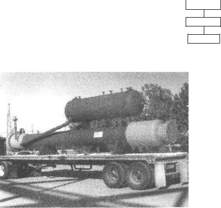
166 |
|
|
|
Steam Generators and Waste Heat Boilers: For Process and Plant Engineers |
|||||||||||||||||||||
|
|
|
|
|
|
|
|
|
|
|
|
|
|
|
|
|
|
|
|
|
|
|
|
||
|
|
|
|
|
|
|
|
|
|
Waste heat boilers |
|
|
|
|
|
|
|
|
|
|
|
||||
|
|
|
|
|
|
|
|
|
|
|
|
|
|
|
|
|
|
|
|
|
|
|
|
|
|
|
|
|
|
|
|
|
|
|
|
|
|
|
|
|
|
|
|
|
|
|
|
|
|
|
|
|
|
|
|
|
|
|
|
|
|
|
|
|
|
|
|
|
|
|
|
|
|
|
|
|
|
|
Gas condition |
|
Purpose |
|
Circulation |
|
|
Firing |
|
|
Steam system |
|
|
Configuration |
|||||||||||
|
|
|
|
|
|
|
|
|
|
|
|
|
|
|
|
|
|
|
|
|
|
|
|
|
|
|
Clean |
|
Process |
|
|
Natural |
|
|
Unfired |
|
|
Multipressure |
|
|
Water tube |
||||||||||
|
|
|
|
|
|
|
|
|
|
|
|
|
|
|
|
|
|
|
|
|
|
|
|
|
|
|
Dirty |
|
Energy recovery |
|
|
Forced |
|
|
Fired |
|
|
Single pressure |
|
|
Fire tube |
||||||||||
|
|
|
|
|
|
|
|
|
|
|
|
|
|
|
|
|
|
|
|
|
|
|
|
|
|
|
Corrosive |
|
|
|
|
|
|
|
|
|
|
|
|
|
|
|
Superheated |
|
|
|
Single pass |
|
|||
|
|
|
|
|
|
|
|
|
|
|
|
|
|
|
|
|
|
|
|
|
|
|
|
|
|
|
Slagging |
|
|
|
|
|
|
|
|
|
|
|
|
|
|
|
Saturated |
|
|
|
Multipass |
|
|||
|
|
|
|
|
|
|
|
|
|
|
|
|
|
|
|
|
|
|
|
|
|
|
|
|
|
Integral drum
Elevated drum
Combination
FIGURE 4.1
Classification of waste heat boilers.
FIGURE 4.2
Fire tube boiler for reformed gas application.
the first and second stages of the superheaters and one between the second stage and final superheater, and one emergency desuperheater at the steam exit to handle sudden fluctuations in steam temperature; the drum also was sized with a large holdup time of about 12 min from normal level to empty. As the flue gas is dusty, a ball cleaning system was incorporated in the second pass in which are located the screen section, superheaters, and evaporator. Steel balls will be dropped over the tube bundles at a frequency determined
Waste Heat Boilers |
167 |
External gas bypass
(a)
Drum
Risers Downcomer
Gas exit
Bypass damper
Gas inert
(b)Internal gas bypass system
FIGURE 4.3
(a) External and (b) internal gas bypass systems.
|
Gas outlet |
|
Steam |
|
drum |
|
abcd |
‘A’ |
Economizer |
|
|
Superheater |
|
|
Gas |
|
|
|
inlet |
abcd |
Evaporator |
abcd |
abcd |
|||
Screen |
|
|
|
section |
|
|
|
|
|
‘A’ |
|
Section “A–A” |
|
Side view |
|
FIGURE 4.4
Water tube waste heat boiler for an incineration plant with screen, superheater, evaporator, and economizer.
by operating conditions, collected at the bottom and sent back to the top of second pass by a pneumatic conveying system (Figure 4.7). Though plain tubes were used for the heating surfaces, the heating surfaces were arranged in a staggered fashion to facilitate better cleaning of tubes. The screen section and evaporator are multistream horizontal tube natural circulation systems. The circulation system was checked carefully considering that horizontal tubes are used in the evaporator. The thermal and performance design of the boiler was done by the author, which was built and erected by a fabricator and is presently in operation in Canada.

168 |
Steam Generators and Waste Heat Boilers: For Process and Plant Engineers |
FIGURE 4.5
Water tube waste heat boiler with furnace section.
Gas Inlet Temperature and Analysis
Inlet gas temperature to the waste heat boiler is an important parameter. Generally, if the inlet gas temperature is above 700°C, a single-pressure heat recovery boiler will be adequate to cool the flue gas to about 130°C–150°C. In gas turbine heat recovery steam generator (HRSG) applications, with a gas inlet temperature of, say, 500°C or in a cement plant with flue gas at 300°C–350°C, we cannot cool the flue gas to 130°C–140°C with mediumor high-pressure steam. This is due to the fact that with practical pinch point limitations (see Chapter 5), the amount of energy recoverable in the superheater and evaporator is fixed. Hence, steam generation is determined by the pinch and approach points. Hence, the lower the inlet gas temperature, the lesser the amount of steam that can be generated with a given pinch point. The economizer water flow equals the steam flow, and hence, the boiler exit gas temperature also falls in place. Thus, lower the inlet gas temperature, lower the steam generation and higher the exit gas temperature and vice versa. That is why multiple-pressure steam generation is required to lower the exhaust gas temperature in HRSGs or cement plants. Single-pressure heat recovery system is adequate when the gas inlet temperature is high. Irrespective of the steam pressure, we can cool the flue gas to about 140°C in oilor gasor solid fuel–fired steam generators with a single-pressure system (the inlet gas temperature may be taken as the adiabatic combustion temperature due to which a large amount of steam is generated in the furnace and evaporator, and hence, the economizer becomes a very large heat sink cooling the flue gas to 130°C–140°C). Alternatively, one has to consider the Kalina system, discussed later, in which a mixture of ammonia–water is used as the working fluid. In this system, the

Waste Heat Boilers |
169 |
||||||||||||||||||||||||||||||||||||||||||||||||||||||
|
|
|
|
|
|
|
|
|
|
|
|
|
|
|
|
|
|
|
|
|
|
|
|
|
|
|
|
|
|
|
|
|
|
|
|
|
|
|
|
|
|
|
|
|
|
|
|
|
|
|
|
|
|
|
|
|
|
|
|
|
|
|
|
|
|
|
|
|
|
|
|
|
|
|
|
|
|
|
|
|
|
|
|
|
|
|
|
|
|
|
|
|
|
|
|
|
|
|
|
|
|
|
|
|
|
|
|
|
|
|
|
|
|
|
|
|
|
|
|
|
|
|
|
|
|
|
|
|
|
|
|
|
|
|
|
|
|
|
|
|
|
|
|
|
|
|
|
|
|
|
|
|
|
|
|
|
|
|
|
|
|
|
|
|
|
|
|
|
|
|
|
|
|
|
|
|
|
|
|
|
|
|
|
|
|
|
|
|
|
|
|
|
|
|
|
|
|
|
|
|
|
|
|
|
|
|
|
|
|
|
|
|
|
|
|
|
|
|
|
|
|
|
|
|
|
|
|
|
|
|
|
|
|
|
|
|
|
|
|
|
|
|
|
|
|
|
|
|
|
|
|
|
|
|
|
|
|
|
|
|
|
|
|
|
|
|
|
|
|
|
|
|
|
|
|
|
|
|
|
|
|
|
|
|
|
|
|
|
|
|
|
|
|
|
|
|
|
|
|
|
|
|
|
|
|
|
|
|
|
|
|
|
|
|
|
|
|
|
|
|
|
|
|
|
|
|
|
|
|
|
|
|
|
|
|
|
|
|
|
|
|
|
|
|
|
|
|
|
|
|
|
|
|
|
|
|
|
|
|
|
|
|
|
|
|
|
|
|
|
|
|
|
|
|
|
|
|
|
|
|
|
|
|
|
|
|
|
|
|
|
|
|
|
|
|
|
|
|
|
|
|
|
|
|
|
|
|
|
|
|
|
|
|
|
|
|
|
|
|
|
|
|
|
|
|
|
|
|
|
|
|
|
|
|
|
|
|
|
|
|
|
|
|
|
|
|
|
|
|
|
|
|
|
|
|
|
|
|
|
|
|
|
|
|
|
|
|
|
|
|
|
|
|
|
|
|
|
|
|
|
|
|
|
|
|
|
|
|
|
|
|
|
|
|
|
|
|
|
|
|
|
|
|
|
|
|
|
|
|
|
|
|
|
|
|
|
|
|
|
|
|
|
|
|
|
|
|
|
|
|
|
|
|
|
|
|
|
|
|
|
|
|
|
|
|
|
|
|
|
|
|
|
|
|
|
|
|
|
|
|
|
|
|
|
|
|
|
|
|
|
|
|
|
|
|
|
|
|
|
|
|
|
|
|
|
|
|
|
|
|
|
|
|
|
|
|
|
|
|
|
|
|
|
|
|
|
|
|
|
|
|
|
|
|
|
|
|
|
|
|
|
|
|
|
|
|
|
|
|
|
|
|
|
|
|
|
|
|
|
|
|
|
|
|
|
|
|
|
|
|
|
|
|
|
|
|
|
|
|
|
|
|
|
|
|
|
|
|
|
|
|
|
|
|
|
|
|
|
|
|
|
|
|
|
|
|
|
|
|
|
|
|
|
|
|
|
|
|
|
|
|
|
|
|
|
|
|
|
|
|
|
|
|
|
|
|
|
|
|
|
|
|
|
|
|
|
|
|
|
|
|
|
|
|
|
|
|
|
|
|
|
|
|
|
|
|
|
|
|
|
|
|
|
|
|
|
|
|
|
|
|
|
|
|
|
|
|
|
|
|
|
|
|
|
|
|
|
|
|
|
|
|
|
|
|
|
|
|
|
|
|
|
|
|
|
|
|
|
|
|
|
|
|
|
|
|
|
|
|
|
|
|
|
|
|
|
|
|
|
|
|
|
|
|
|
|
|
|
|
|
|
|
|
|
|
|
|
|
|
|
|
|
|
|
|
|
|
|
|
|
|
|
|
|
|
|
|
|
|
|
|
|
|
|
|
|
|
|
|
|
|
|
|
|
|
|
|
|
|
|
|
|
|
|
|
|
|
|
|
|
|
|
|
|
|
|
|
|
|
|
|
|
|
|
|
|
|
|
|
|
|
|
|
|
|
|
|
|
|
|
|
|
|
|
|
|
|
|
|
|
|
|
|
|
|
|
|
|
|
|
|
|
|
|
|
|
|
|
|
|
|
|
|
|
|
|
|
|
|
|
|
|
|
|
|
|
|
|
|
|
|
|
|
|
|
|
|
|
|
|
|
|
|
|
|
|
|
|
|
|
|
|
|
|
|
|
|
|
|
|
|
|
|
|
|
|
|
|
|
|
|
|
|
|
|
|
|
|
|
|
|
|
|
|
|
|
|
|
|
|
|
|
|
|
|
|
|
|
|
|
|
|
|
|
|
|
|
|
|
|
|
|
|
|
|
|
|
|
|
|
|
|
|
|
|
|
|
|
|
|
|
|
|
|
|
|
|
|
|
|
|
|
|
|
|
|
|
|
|
|
|
|
|
|
|
|
|
|
|
|
|
|
|
|
|
|
|
|
|
|
|
|
|
|
|
|
|
|
|
|
|
|
|
|
|
|
|
|
|
|
|
|
|
|
|
|
|
|
|
|
|
|
|
|
|
|
|
|
|
|
|
|
|
|
|
|
|
|
|
|
|
|
|
|
|
|
|
|
|
|
|
|
|
|
|
|
|
|
|
|
|
|
|
|
|
|
|
|
|
|
|
|
|
|
|
|
|
|
|
|
|
|
|
|
|
|
|
|
|
|
|
|
|
|
|
|
|
|
|
|
|
|
|
|
|
|
|
|
|
|
|
|
|
|
|
|
|
|
|
|
|
|
|
|
|
|
|
|
|
|
|
|
|
|
|
|
|
|
|
|
|
|
|
|
|
|
|
|
|
|
|
|
|
|
|
|
|
|
|
|
|
|
|
|
|
|
|
|
|
|
|
|
|
|
|
|
|
|
|
|
|
|
|
|
|
|
|
|
|
|
|
|
|
|
|
|
|
|
|
|
|
|
|
|
|
|
|
|
|
|
|
|
|
|
|
|
|
|
|
|
|
|
|
|
|
|
|
|
|
|
|
|
|
|
|
|
|
|
|
|
|
|
|
|
|
|
|
|
|
|
|
|
|
|
|
|
|
|
|
|
|
|
|
|
|
|
|
|
|
|
|
|
|
|
|
|
|
|
|
|
|
|
|
|
|
|
|
|
|
|
|
|
|
|
|
|
|
|
|
|
|
|
|
|
|
|
|
|
|
|
|
|
|
|
|
|
|
|
|
|
|
|
|
|
|
|
|
|
|
|
|
|
|
|
|
|
|
|
|
|
|
|
|
|
|
|
|
|
|
|
|
|
|
|
|
|
|
|
|
|
|
|
|
|
|
|
|
|
|
|
|
|
|
|
|
|
|
|
|
|
|
|
|
|
|
|
|
|
|
|
|
|
|
|
|
|
|
|
|
|
|
|
|
|
|
|
|
|
|
|
|
|
|
|
|
|
|
|
|
|
|
|
|
|
|
|
|
|
|
|
|
|
|
|
|
|
|
|
|
|
|
|
|
|
|
|
|
|
|
|
|
|
|
|
|
|
|
|
|
|
|
|
|
|
|
|
|
|
|
|
|
|
|
|
|
|
|
|
|
|
|
|
|
|
|
|
|
|
|
|
|
|
|
|
|
|
|
|
|
|
|
|
|
|
|
|
|
|
|
|
|
|
|
|
|
|
|
|
|
|
|
|
|
|
|
|
|
|
|
|
|
|
|
|
|
|
|
|
|
|
|
|
|
|
|
|
|
|
|
|
|
|
|
|
|
|
|
|
|
|
|
|
|
|
|
|
|
|
|
|
|
|
|
|
|
|
|
|
|
|
|
|
|
|
|
|
|
|
|
|
|
|
|
|
|
|
|
|
|
|
|
|
|
|
|
|
|
|
|
|
|
|
|
|
|
|
|
|
|
|
|
|
|
|
|
|
|
|
|
|
|
|
|
|
|
|
|
|
|
|
|
|
|
|
|
|
|
|
|
|
|
|
|
|
|
|
|
|
|
|
|
|
|
|
|
|
|
|
|
|
|
|
|
|
|
|
|
|
|
|
|
|
|
|
|
|
|
|
|
|
|
|
|
|
|
|
|
|
|
|
|
|
|
|
|
|
|
|
|
|
|
|
|
|
|
|
|
|
|
|
|
|
|
|
|
|
|
|
|
|
|
|
|
|
|
|
|
|
|
|
|
|
|
|
|
|
|
|
|
|
|
|
|
|
|
|
|
|
|
|
|
|
|
|
|
|
|
|
|
|
|
|
|
|
|
|
|
|
|
|
|
|
|
|
|
|
|
|
|
|
|
|
|
|
|
|
|
|
|
|
|
|
|
|
|
|
|
|
|
|
|
|
|
|
|
|
|
|
|
|
|
|
|
|
|
|
|
|
|
|
|
|
|
|
|
|
|
|
|
|
|
|
|
|
|
|
|
|
|
|
|
|
|
|
|
|
|
|
|
|
|
|
|
|
|
|
|
|
|
|
|
|
|
|
|
|
|
|
|
|
|
|
|
|
|
|
|
|
|
|
|
|
|
|
|
|
|
|
|
|
|
|
|
|
|
|
|
|
|
|
|
|
|
|
|
|
|
|
|
|
|
|
|
|
|
|
|
|
|
|
|
|
|
|
|
|
|
|
|
|
|
|
|
|
|
|
|
|
|
|
|
|
|
|
|
|
|
|
|
|
|
|
|
|
|
|
|
|
|
|
|
|
|
|
|
|
|
|
|
|
|
|
|
|
|
|
|
|
|
|
|
|
|
|
|
|
|
|
|
|
|
|
|
|
|
|
|
|
|
|
|
|
|
|
|
|
|
|
|
|
|
|
|
|
|
|
|
|
|
|
|
|
|
|
|
|
|
|
|
|
|
|
|
|
|
|
|
|
|
|
|
|
|
|
|
|
|
|
|
|
|
|
|
|
|
|
|
|
|
|
|
|
|
|
|
|
|
|
|
|
|
|
|
|
|
|
|
|
|
|
|
|
|
|
|
|
|
|
|
|
|
|
|
|
|
|
|
|
|
|
|
|
|
|
|
|
|
|
|
|
|
|
|
|
|
|
|
|
|
|
|
|
|
|
|
|
|
|
|
|
|
|
|
|
|
|
|
|
|
|
|
|
|
|
|
|
|
|
|
|
|
|
|
|
|
|
|
|
|
|
|
|
|
|
|
|
|
|
|
|
|
|
|
|
|
|
|
|
|
|
|
|
|
|
|
|
|
|
|
|
|
|
|
|
|
|
|
|
|
|
|
|
|
|
|
|
|
|
|
|
|
|
|
|
|
|
|
|
|
|
|
|
|
|
|
|
|
|
|
|
|
|
|
|
|
|
|
|
|
|
|
|
|
|
|
|
|
|
|
|
|
|
|
|
|
|
|
|
|
|
|
|
|
|
|
|
|
|
|
|
|
|
|
|
|
|
|
|
|
|
|
|
|
|
|
|
|
|
|
|
|
|
|
|
|
|
|
|
|
|
|
|
|
|
|
|
|
|
|
|
|
|
|
|
|
|
|
|
|
|
|
|
|
|
|
|
|
|
|
|
|
|
|
|
|
|
|
|
|
|
|
|
|
|
|
|
|
|
|
|
|
|
|
|
|
|
|
|
|
|
|
|
|
|
|
|
|
|
|
|
|
|
|
|
|
|
|
|
|
|
|
|
|
|
|
|
|
|
|
|
|
|
|
|
|
|
|
|
|
|
|
|
|
|
|
|
|
|
|
|
|
|
|
|
|
|
|
|
|
|
|
|
|
|
|
|
|
|
|
|
|
|
|
|
|
|
|
|
|
|
|
|
|
|
|
|
|
|
|
|
|
|
|
|
|
|
|
|
|
|
|
|
|
|
|
|
|
|
|
|
|
|
|
|
|
|
|
|
|
|
|
|
|
|
|
|
|
|
|
|
|
|
|
|
|
|
|
|
|
|
|
|
|
|
|
|
|
|
|
|
|
|
|
|
|
|
|
|
|
|
|
|
|
|
|
|
|
|
|
|
|
|
|
|
|
|
|
|
|
|
|
|
|
|
|
|
|
|
|
|
|
|
|
|
|
|
|
|
|
|
|
|
|
|
|
|
|
|
|
|
|
|
|
|
|
|
|
|
|
|
|
|
|
|
|
|
|
|
|
|
|
|
|
|
|
|
|
|
|
|
|
|
|
|
|
|
|
|
|
|
|
|
|
|
|
|
|
|
|
|
|
|
|
|
|
|
|
|
|
|
|
|
|
|
|
|
|
|
|
|
|
|
|
|
|
|
|
|
|
|
|
|
|
|
|
|
|
|
|
|
|
|
|
|
|
|
|
|
|
|
|
|
|
|
|
|
|
|
|
|
|
|
|
|
|
|
|
|
|
|
|
|
|
|
|
|
|
|
|
|
|
|
|
|
|
|
|
|
|
|
|
|
|
|
|
|
|
|
|
|
|
|
|
|
|
|
|
|
|
|
|
|
|
|
|
|
|
|
|
|
|
|
|
|
|
|
|
|
|
|
|
|
|
|
|
|
|
|
|
|
|
|
|
|
|
|
|
|
|
|
|
|
|
|
|
|
|
|
|
|
|
|
|
|
|
|
|
|
|
|
|
|
|
|
|
|
|
|
|
|
|
|
|
|
|
|
|
|
|
|
|
|
|
|
|
|
|
|
|
|
|
|
|
|
|
|
|
|
|
|
|
|
|
|
|
|
|
|
|
|
|
|
|
|
|
|
|
|
|
|
|
|
|
|
|
|
|
|
|
|
|
|
|
|
|
|
|
|
|
|
|
|
|
|
|
|
|
|
|
|
|
|
|
|
|
|
|
|
|
|
|
|
|
|
|
|
|
|
|
|
|
|
|
|
|
|
|
|
|
|
|
|
|
|
|
|
|
|
|
|
|
|
|
|
|
|
|
|
|
|
|
|
|
|
|
|
|
|
|
|
|
|
|
|
|
|
|
|
|
|
|
|
|
|
|
|
|
|
|
|
|
|
|
|
|
|
|
|
|
|
|
|
|
|
|
|
|
|
|
|
|
|
|
|
|
|
|
|
|
|
|
|
|
|
|
|
|
|
|
|
|
|
|
|
|
|
|
|
|
|
|
|
|
|
|
|
|
|
|
|
|
|
|
|
|
|
|
|
|
|
|
|
|
|
|
|
|
|
|
|
|
|
|
|
|
|
|
|
|
|
|
|
|
|
|
|
|
|
|
|
|
|
|
|
|
|
|
|
|
|
|
|
|
|
|
|
|
|
|
|
|
|
|
|
|
|
|
|
|
|
|
|
|
|
|
|
|
|
|
|
|
|
|
|
|
|
|
|
|
|
|
|
|
|
|
|
|
|
|
|
|
|
|
|
|
|
|
|
|
|
|
|
|
|
|
|
|
|
|
|
|
|
|
|
|
|
|
|
|
|
|
|
|
|
|
|
|
|
|
|
|
|
|
|
|
|
|
|
|
|
|
|
|
FIGURE 4.6
Water tube waste heat boiler for a steel mill kiln. (Courtesy of Elkam, Alma, Quebec, Canada.)
working fluid has variable boiling points unlike steam, and the exhaust gas can be cooled to a much lower temperature compared to a steam system even if the inlet gas temperature is around 200°C–250°C.
The need for multiple-pressure steam is also discussed in Chapter 5. Depending on the ratio of HP steam to LP steam flow or the ratio of HP to LP steam pressure, one decides if

170 |
Steam Generators and Waste Heat Boilers: For Process and Plant Engineers |
2 |
4 |
2 |
|||
|
|
|
|
|
|
|
|
|
|
|
|
|
|
|
|
|
|
|
|
|
|
|
|
3 |
3 |
|
|
1 |
|
1 |
|
|
|
||
|
|
Shot cleaning system: |
|
|
|
1—Tube bank |
|
|
|
2—Shot feeding chamber |
|
|
|
3—Shot spreader |
|
10 |
|
4—Transport air outlet |
|
6 |
|
5—Air for dust/shot separation |
|
5 |
7 |
6—Separator/shot collector |
|
6 |
7—Strainer |
||
|
|||
9 |
|
8—Shot transport nozzle |
|
8 |
|
9—Transport air fan |
|
|
|
10—Diverting ba‚e
FIGURE 4.7
Shot cleaning system for waste heat boiler.
singleor multipressure HRSG is required. Generally speaking, multiple-pressure steam generation is required when gas inlet temperature is low, on the order of 500°C or less.
Flue Gas Composition and Gas Pressure
Flue gas analysis is important to the design of the boiler. A large amount of water vapor or hydrogen increases the gas specific heat and thermal conductivity and hence the gas and overall heat transfer coefficient, boiler duty, and heat flux. Presence of SO2 lowers the gas specific heat and hence the duty. For example, in hydrogen plant reformed gas boilers where we have a large % volume of hydrogen and water vapor in the flue gas at high gas pressure, the heat transfer coefficient can be five to eight times that of typical flue gas from the combustion of natural gas. Heat flux is a concern in these applications.
The presence of chlorine and hydrogen chloride vapor in flue gas is indicative of corrosion potential particularly if a superheater is used and the tube wall temperature is above 475°C. Chlorine attacks carbon steel even at low temperatures as shown in Figure 4.8. Hence, low-pressure saturated steam is generated with flue gas containing chlorine and economizers are avoided. Presence of hydrogen chloride gas (HCl) also indicates hightemperature corrosion. There are instances of high-temperature stainless steel superheaters in several municipal solid waste incineration plants having been destroyed within a few months of operation due to HCl. Hence, modular municipal solid waste incineration plants generate steam at medium pressure and low temperature (about 40 barg, 375°C) enabling longer life of superheater tubes.

Waste Heat Boilers |
|
|
|
|
171 |
||
Corrosion rate |
|
|
Dry chlorine |
|
|
Dry HCl |
|
|
|
|
|
||||
|
|
|
|
|
|
|
|
|
|
|
|
|
|
|
|
200 |
400 |
600 |
800 |
1000 |
1200 |
|
|
|
|
|
Metal temperature, °F |
|
|
|
|
FIGURE 4.8
Chlorine and hydrogen chloride in flue gas cause corrosion problems.
The presence of SO3 and HCl in the flue gas also suggests low-temperature corrosion problems due to the acid vapor condensation. To minimize low-temperature corrosion concerns, there are several methods that are discussed in Chapter 3. Major decisions such as using membrane wall construction or refractory-lined casing depend on the flue gas analysis and dew point of the flue gas and cost considerations.
More care should be taken when the flue gas contains ash, which has slagging potential. This is common in steel plant effluents or municipal solid waste incineration systems. A furnace to cool the flue gas to below the ash melting temperature as shown in Figure 4.5 or Figure 4.6 is one solution. Some plants recirculate flue gas from the boiler rear and lower the gas inlet temperature to the boiler below the ash melting temperatures. However, this increases the flue gas quantity through the boiler and increases the gas pressure drop, or the boiler cross section may have to be increased. Double-spaced screen section, which prevents molten ash from sticking to the boiler tubes, is recommended, if slagging is envisaged. Tube spacing of 150–200 mm is used at the convective bank inlet as shown for a few rows deep. One can gradually reduce the tube spacing as the gas cools. The superheater, which is more prone to corrosion when deposits stick on to them, is located in a much cooler zone by using adequate number of screen tubes ahead of it.
Flue gas pressure is generally atmospheric in many applications; in pressurized systems (such as gas turbine HRSGs or incineration plants), the flue gas is well contained in the boiler if a membrane wall construction is used. If a suction system with an induced draft fan is used as in some biomass heat recovery projects, then there is possibility of leakage of cold air from the atmosphere into the boiler through man-way doors or hopper openings. This is likely to affect local gas temperatures, and hence, performance prediction may not be accurate. Superheated steam temperature may also be impacted by ingress of cold air into the system.
In reformed gas boilers in hydrogen plants or nitric acid plants, the gas pressure can be very high and hence fire tube boilers are preferred, though special water tube boilers have been built. Table 4.1 shows the flue gas analysis and pressure for different waste gas [1] streams. Alloy steel tubes are recommended when hydrogen is present in flue gas; hence, reformed gas boilers use T11 or T22 tubes for the evaporator to minimize high-temperature concerns. Nelsons chart is often referred to for material selection (Figure 4.9).
In incineration systems involving halogenated compounds, one has to ensure that the combustion temperature of 850°C–900°C is maintained for at least 2 s in the incinerator combustion chamber to destroy the formation of dioxins. Following combustion, the flue

172 |
|
Steam Generators and Waste Heat Boilers: For Process and Plant Engineers |
|||||||||||
|
TABLE 4.1 |
|
|
|
|
|
|
|
|
|
|
|
|
|
Analysis of Waste Gases from Process Plants, % Volume |
|
|
|
|
|
|
||||||
|
|
|
|
|
|
|
|
|
|
|
|
|
|
|
Gas |
1 |
2 |
3 |
4 |
5 |
6 |
7 |
8 |
9 |
10 |
11 |
|
|
|
|
|
|
|
|
|
|
|
|
|
|
|
|
CO2 |
3 |
|
|
9 |
6 |
12 |
7 |
6 |
|
28 |
0 |
|
|
H2O |
7 |
|
|
18 |
37 |
10 |
8 |
23 |
19 |
7 |
1 |
|
|
N2 |
75 |
80 |
81 |
70 |
.5 |
72 |
76 |
55 |
66 |
59.5 |
78 |
|
|
O2 |
15 |
10 |
11 |
3 |
|
6 |
4 |
|
6 |
5.5 |
21 |
|
|
SO2 |
|
10 |
1 |
|
|
|
|
6 |
|
|
|
|
|
HCl |
|
|
|
|
|
|
5 |
|
|
|
|
|
|
SO3 |
|
|
7 |
|
|
|
|
|
|
|
|
|
|
CO |
|
|
|
|
8 |
|
|
3 |
|
|
|
|
|
CH4 |
|
|
|
|
5.5 |
|
|
|
|
|
|
|
|
H2S |
|
|
|
|
|
|
|
3 |
|
|
|
|
|
H2 |
|
|
|
|
43 |
|
|
4 |
|
|
|
|
|
NO |
|
|
|
|
|
|
|
|
9 |
|
|
|
|
Press., atm |
1 |
1 |
1 |
1 |
30–50 |
1 |
1 |
1.5 |
3–10 |
1 |
1 |
|
|
Temp., °C |
600– |
1000– |
500– |
1100– |
1100– |
1000– |
1350– |
1400– |
850– |
450– |
400– |
|
|
|
100 |
300 |
250 |
200 |
300 |
200 |
250 |
350 |
250 |
150 |
100 |
|
Notes: (1) Gas turbine exhaust, (2) raw sulfur gases, (3) SO3 gases after converter, (4) reformer flue gas,
(5) reformed gas, (6) MSW incinerator exhaust, (7) chlorinated plastics incineration, (8) sulfur condenser effluent, (9) nitrous gases, (10) preheater effluent—cement plant, (11) clinker cooler effluent—cement plant.
|
|
|
|
|
Surface |
|
|
1300 |
|
|
|
decarburization |
|
|
|
|
|
|
|
|
|
1100 |
|
|
|
6% Cr 0.5% Mo |
|
°F |
|
|
|
|
3% Cr 0.5% Mo |
|
|
1.25% Cr 0.5% Mo |
|
|
|||
Temperature, |
900 |
|
|
|
||
|
|
|
2% Cr 0% Mo |
|
||
|
|
|
|
|
||
700 |
Not welded |
|
|
0.5% Mo |
||
|
|
|
|
|
||
|
500 |
Welded |
|
|
|
0.25% Mo |
|
|
|
Carbon steel |
|
|
|
|
300 |
or hot formed |
|
|
|
|
|
|
|
|
|
||
|
500 |
1000 |
1500 |
2000 |
2500 |
|
|
0 |
|||||
Hydrogen partial pressure, psia
FIGURE 4.9
Nelson’s chart for the selection of materials.
gas should be cooled very quickly in the waste heat boiler, typically in less than 0.5 s to ensure dioxins are not formed. Finned water tube boilers have shorter gas path and hence shorter residence time. With fire tube boilers, the residence time may be longer and has to be checked. One option as we shall see later is to use smaller-diameter tubes in fire tube boilers to reduce their length.
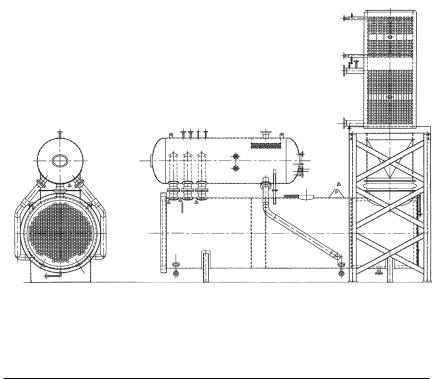
Waste Heat Boilers |
173 |
Water Tube versus Fire Tube Boilers
A common classification of boilers is whether the gas flows inside the tubes as in fire tube boilers (Figure 4.10) or outside the tubes as in water tube boilers (Figure 4.5). The features of each type are discussed in Table 4.2 [2].
Generally, water tube boilers are suitable for large gas flows in the range of millions of kg/h and can handle high steam pressures and temperatures. Fire tube boilers are suitable for low steam pressures generally below 3500 kPa (35 bar) and low gas flows. Table 4.3 shows the effect of pressure on tube thickness for both types. A given tube thickness can withstand about twice the pressure when it is inside than when outside. Hence, fire tube boilers require large thickness as the steam pressure increases and thus become uneconomical;
Economizer
Superheater
FIGURE 4.10
Fire tube boiler with superheater and economizer. (Courtesy of ABCO Industries, Abilene, TX.)
TABLE 4.2
Comparison of Fire Tube and Water Tube Boilers
Item |
Fire Tube |
Water Tube |
|
|
|
Gas flow |
Small—less than 30,000 kg/h |
Large—30,000–1,000,000 kg/h |
Gas inlet temperature |
Low to adiabatic combustion |
Low to adiabatic combustion |
Gas pressure |
As high as 150 barg |
500–1000 mm wc |
Firing |
Possible |
Possible |
Type of heating surface |
Plain tubes |
Plain and finned tubes |
Superheater location |
At inlet or exit |
Anywhere in the gas path |
Water inventory |
High |
Low |
Heat flux on steam side |
Generally low |
Can be high with finned tubes |
Multiple pressure |
No |
Yes |
Multiple modules |
No |
Yes |
Soot blower location |
Inlet or exit |
Anywhere in gas path |
|
|
|
174 |
Steam Generators and Waste Heat Boilers: For Process and Plant Engineers |
|||
|
TABLE 4.3 |
|
|
|
|
Tube Thickness versus Steam Pressure |
|
|
|
|
|
|
|
|
|
Tube Thickness, mm |
External Pressure, barg |
Internal Pressure, barg |
|
|
|
|
|
|
|
2.7 |
40 |
79 |
|
|
3.05 |
47.3 |
92.3 |
|
|
3.5 |
55 |
106 |
|
|
3.9 |
63.5 |
119 |
|
|
4.6 |
81 |
147 |
|
Note: 50.8 mm SA 192, SA 178a carbon steel tubes at 371°C.
they also get huge and heavy as plain tubes are used unlike water tube boilers where finned tubes are used to make the boilers compact.
Sometimes, a combination of fire tube and water tube boilers may be required. Figure 4.11 shows a waste heat boiler for a small hydrogen plant cooling both the furnace flue gas and the reformed gas. The reformed gas is at a high gas pressure and hence a fire tube boiler is appropriate, while the clean flue gas is at atmospheric pressure and a water tube boiler with extended surface is ideal. Since the gas flows and steam generation are small, a compact package unit as shown was designed and built.
Water tube boilers weigh less as they can be made compact using finned tubes (see Appendix E on finned tubes). One may install superheaters even in fire tube boilers, but the location is either at the inlet or exit (Figure 4.10). It may be installed at the turnaround section between the second and third gas passes also as discussed in Chapter 3. In any case compared to water tubes, these locations may not be the optimum. If the flue gas is slagging in nature, a water tube boiler with cleaning devices is a better choice compared to a fire tube boiler as the tube inlet will be plugged up with slag in a fire tube unit and cleaning will be required at a greater frequency.
Multiple-pressure steam generation is required to lower the exit gas temperature if the inlet gas temperature is low. This point will be illustrated with calculations in Chapter 5 on HRSG simulation. While multiple-pressure modules are easy to build with water tube boilers, they are rarely seen with fire tubes as it is uneconomical and space requirement will be huge.
Circulation Systems
There can be a variety of circulation systems involving waste heat boilers depending on whether they are fire tube or water tube and whether they have single or multiple evaporators. Figure 4.10 shows a fire tube boiler with external steam drum, downcomers, and risers. Figure 4.11 shows a combination of fire tube and water tube with circulation system. Figure 4.4 shows a water tube boiler with screen and evaporator sections with a superheater in between. The screen and evaporator sections operate in parallel and are connected to the same steam drum by external downcomers and risers. Figure 4.12 shows two fire tube boilers sharing the same steam drum. Figure 4.6 shows a water tube boiler in which the screen section and evaporator sections have multistream horizontal tubes and are connected to the same steam drum by external downcomers and risers. Figure 2.13d shows a large evaporator that required an external steam drum and hence external downcomers, risers, are used.
Circulation calculations are quite involved and preferably done using a computer program as numerous iterations are required before one can arrive at the circulation ratio

Waste Heat Boilers |
175 |
Flue gas
Feed gas heater
Steam drum
Flue gas boiler
Reformed
gas boiler
FIGURE 4.11
Combination fire tube and water tube design.
(CR), which is based on the resistance of the downcomers, risers, and evaporator tubes, and the drum location. The procedure is explained in Chapter 2. A forced circulation steam generator using circulation pumps is shown in Chapter 2, while Chapter 3 shows a forced circulation system for an oil field steam generator.
Table 4.4 shows the results from a computer program for the circulation system involving boiler with screen section that has horizontal tubes and multiple streams (Figure 4.6). The screen section generates 13,150 kg/h in the maximum case. It has a screen section with 160 streams (parallel paths); each tube has a developed length of 12.2 m. The distance between the drum centerline and bottom of screen is 5.34 m. There are two downcomers of inner diameter 150 mm and two external risers of inner diameter 190 mm. Their lengths are about 8 m. As discussed in Chapter 2, the CR was assumed, and the various singleand two-phase flow losses were computed, and iterations were carried out till the available head matched the losses as shown. The CR finally arrived at is 12.45.

176 |
Steam Generators and Waste Heat Boilers: For Process and Plant Engineers |
Steam
drum
First pass |
Second pass |
|
FIGURE 4.12
Fire tube boilers with common steam drum.
With horizontal tubes, one has to also check if flow stagnation is likely. Froude number is an indicator of inertial forces to gravity forces, and if it is above 0.04, flow separation is unlikely.
Froude number F = G2/(ρ2gd)
where
G is the mass flow inside the tubes (liquid only), kg/m2 s ρ is the density of liquid (807 kg/m3)
g is the acceleration due to gravity (9.8 m/s2) d is the tube inner diameter (0.026 m)
In this example, the liquid-only mass flow = (1 − 1/CR) × 13,150 × 12.45 = 0.92 × 13,150 × 12.45 = 150,620 kg/h
G = mass velocity = 150620 × 4/(π × 0.026 × 0.026 × 160)/3600 = 493 kg/m2s
F = 493 × 493/(807 × 807 × 9.8 × 0.026) = 1.46. As this is much higher than the limiting value of 0.04, stagnation is unlikely. The said boiler has been operating well for the past few years. A few boiler suppliers use inclined horizontal tubes to provide a better comfort factor for the flow of two-phase mixture inside tubes at medium and high steam pressures (Figure 4.22c, later in the chapter).
When a circulation pump is used as in forced circulation, boilers the CR is predetermined, say, 4–8 and the circulating pump differential head is selected based on water flow corresponding to CR selected; the pump head is obtained after checking the available head and computing the losses.
TABLE 4.4
Circulation Calculations
Screen Section
Steam pressure |
37 |
kg/cm2g |
|
|
|
|
|
|
|
|
|
Sat. temperature |
244 |
°C |
|
|
|
|
|
|
|
|
|
Feed water temp. |
204 |
°C |
|
|
|
|
|
|
|
|
|
Sp. vol. steam |
0.0650 |
m3/kg |
|
|
|
|
|
|
|
|
|
Sp. vol. water |
0.0012 |
m3/kg |
|
|
|
|
|
|
|
|
|
Average CR |
12.46 |
|
|
|
|
|
|
|
|
|
|
Total static head |
5.34 |
m |
|
|
|
|
|
|
|
|
|
Total static head |
0.44 |
kg/cm2 |
|
|
|
|
|
|
|
|
|
Downcomer losses |
0.04 |
kg/cm2 |
|
|
|
|
|
|
|
|
|
Riser losses |
0.06 |
kg/cm2 |
|
|
|
|
|
|
|
|
|
Riser gravity loss |
0 12 |
kg/cm2 |
|
|
|
|
|
|
|
|
|
Drum internals’ loss |
0 07 |
kg/cm2 |
|
|
|
|
|
|
|
|
|
Mixture temp. |
242 |
°C |
|
|
|
|
|
|
|
|
|
|
|
|
|
|
|
|
|
|
Press. |
|
|
Path |
Level |
Sort |
Diameter |
Length |
Bends |
Flow |
Velocity |
No. Tubes |
Drop |
Internal dc |
|
1 |
1 |
1 |
150 |
8 |
3 |
163,718 |
1.56 |
2 |
0.04 |
Downcomer |
|
1 |
1 |
1 |
190 |
8.5 |
3 |
163,718 |
4.37 |
2 |
0.06 |
Riser |
|
Stream flow |
Quality |
Accln. loss |
Gravity |
Friction |
Total flow |
Tubes |
Tube ID |
Boiling ht. |
Length |
CR |
Boiling ht. |
|
|
|
loss |
loss |
|
|
|
|
|
|
|
13,150 |
0.079 |
0.007 |
0.061 |
0.082 |
164,100 |
160 |
26.00 |
1.2 |
12.20 |
12.7 |
0.4 |
kg/h |
|
kg/cm2 |
|
|
kg/h |
|
mm |
m |
m |
|
m |
Boilers Heat Waste
177

178 |
Steam Generators and Waste Heat Boilers: For Process and Plant Engineers |
Heat Recovery in Sulfur Plants
A sulfur plant forms an important part of a gas processing system in a refinery or gas processing plants. Sulfur is present in natural gas as hydrogen sulfide (H2S); it is the by-product of processing natural gas and refining high-sulfur crude oils. For process and combustion applications, the sulfur in the natural gas has to be removed. Sulfur recovery refers to the conversion of hydrogen sulfide to elemental sulfur. The most common process for sulfur removal is the Claus process, which recovers about 95%–97% of the H2S in the feed stream (Figure 4.13). Waste heat boilers are an important part of this process (Figure 4.14a). Due to low gas inlet temperature in sulfur condenser, a single-shell fire tube boiler is often used.
The Claus process used today is a modification of a process first used in 1883, in which H2S was reacted over a catalyst with air to form elemental sulfur and water. The reaction is expressed as follows:
H2S + 1/2O2 → S + H2O
Control of this exothermic reaction was difficult, and sulfur recovery efficiency was low. Modifications later included burning a third of the H2S to produce SO2, which is reacted with the remaining H2S to produce elemental sulfur; this process consists of multistage catalytic oxidation of H2S according to the reactions:
2H2S + 3O2 → 2SO2 + 2H2O + heat
2H2S + O2 → 2S + 2H2O
Each catalytic stage consists of a gas reheater, a catalyst chamber, and a sulfur condenser as shown in Figure 4.14. In addition to the oxidation of H2S to SO2 and the reaction of SO2 with H2S in the reaction furnace, many other side reactions occur to yield gas stream containing
CO2, H2S, SO2, H2, CH4, and H2O in addition to various species of sulfur. The duty of the boiler behind the sulfur combustor includes both sensible heat from cooling of gas stream
from 1426°C (2600°F) to 343°C (650°F) and the duty associated with the transformation of
|
|
|
|
|
|
|
|
|
|
|
|
|
|
|
|
|
|
|
|
|
|
|
|
|
|
|
|
|
|
|
|
|
|
|
HP steam |
|
|
|
|
|
|
|
|
Converter 1 |
|
|
|
|
|
|
|
Converter 2 |
|
|
|
||||||||
|
|
|
|
|
|
|
|
|
|
|
|
|
|
|
|
|
|
|
|
|
|||||||||||
|
|
|
|
|
|
|
|
|
|
|
|
|
|
|
|
|
|
|
|
|
|
|
|
|
|
|
|
|
|
||
|
|
|
|
|
|
|
|
|
|
|
|
|
|
|
|
|
|
|
|
|
|
|
|
|
|
|
|
|
|
|
|
|
|
|
|
|
|
|
|
Reheater |
1 |
|
|
|
|
|
|
|
|
|
|
|
|
|
|||||||||
|
|
|
|
|
|
|
|
|
|
|
|
|
Reheater |
2 |
|
|
|
|
|
|
|
|
|
||||||||
|
|
|
|
|
Acid gas |
|
|
|
|
Acid gas |
|
|
|
|
|
|
|
|
|
Tail gas |
|||||||||||
|
|
|
WHB |
|
|
|
|
|
|
|
|
|
|
|
|||||||||||||||||
|
|
|
|
|
|
|
|
|
|
|
|
|
|
|
|
|
|
|
|
|
|
|
|
|
|
||||||
|
|
|
|
Air |
|
|
|
|
|
|
Air |
|
|
|
|
|
|
|
|
|
|
||||||||||
|
|
|
|
|
|
|
|
|
|
|
|
|
|
|
|
|
|
|
|
|
|
|
|
LP steam |
|
|
|||||
|
|
|
|
|
|
|
LP steam |
|
|
LP steam |
|
|
|
|
|||||||||||||||||
|
|
|
|
|
|
|
|
|
|
|
|
|
|
|
|
|
|
|
|
|
|
|
|
|
|
|
|
|
|
|
|
|
|
|
|
|
|
|
|
|
|
|
|
|
|
|
|
|
|
|
|
|
|
|
|
|
|
|
|
|
|
|
|
Air |
BFW |
|
|
WHB |
|
|
|
WHB |
|
|
|
|
WHB |
||||||||||||||||||
|
|
|
|
|
|
|
|
|
|
|
|||||||||||||||||||||
|
|
|
|
|
|
|
|
|
|
|
|
|
|
||||||||||||||||||
Acid gas
|
|
|
|
|
|
|
|
|
|
|
|
Ko drum |
|
|
|
|
|
|
|
|
BFW |
||
BFW |
|
|
BFW |
|
|
|
|
|
|||
|
|
|
|
|
|
|
|
|
|
|
|
|
|
|
|
|
|
|
|
|
|
|
|
Sulfur pit
FIGURE 4.13
Claus process for sulfur recovery.

Waste Heat Boilers |
179 |
(a)
Multipass tube-side arrangement
Sulfur condenser
(b)
FIGURE 4.14
(a) Two-pass fire tube waste heat boiler for Claus plant. (b) Sulfur condenser with multistreams from reaction generating low-pressure steam.
various species of sulfur. The reaction furnace operates at 982°C–1537°C (1800°F–2800°F), and the flue gas is passed through a waste heat boiler in which saturated steam at about 40 barg is generated. This is typically a two–gas pass design, though single-pass designs are available. The gas is cooled to 650°C (1200°F) in the first pass and finally to 343°C in the second pass.
Figure 4.12 shows the boiler for a large sulfur recovery plant, which consists of two separate shells one for each pass connected to a common steam drum. The external down- comer–riser system ensures adequate circulation and cooling of the tube sheet, which is refractory lined. Ceramic ferrules are used to protect the tube-to-tube sheet joint, as shown in Figure 4.15. The inlet gas chamber is also refractory lined. The casing is kept between 175°C and 205°C (350°F–400°F) through a combination of internal and external insulation

180 |
Steam Generators and Waste Heat Boilers: For Process and Plant Engineers |
Insulation |
Tube |
Tube sheet
Gas in
Ferrule
(a)
(b)
FIGURE 4.15
(a) Tube to tube sheet joint. (b) Picture of tube sheet with refractory and ferrules. (Courtesy of Cleaver Brooks, Thomasville, GA.)
to minimize concerns regarding acid dew point corrosion. The exit chamber is externally insulated. About 65%–70% of the sulfur is removed in the boiler as liquid sulfur by using heated drains. Figure 4.14b shows a single-pass design for the same application. The purpose of using ferrules is explained later. Refractory on tube sheet and ferrules reduce the heat flux through the tube sheet and hence keep the tube sheet cool. Calculations for tube sheet temperature are shown later with and without tube sheet refractory and ferrules.

Waste Heat Boilers |
181 |
Though the boiler operates above the sulfur dew point, some sulfur may condense at partial loads and during transient start-up or shutdown mode. The cooled gases exiting the exchanger are reheated to maintain acceptable reaction rates and to ensure that process gases remain above the sulfur dew point and are sent to the catalyst beds for further conversion as shown in Figure 4.13. The catalytic reactors using alumina or bauxite catalysts operate at lower temperatures ranging from 200°C to 315°C. Because this reaction represents an equilibrium chemical reaction, it is not possible for a Claus plant to convert all of the incoming sulfur to elemental sulfur. Therefore, two or more stages are used. Each catalytic stage can recover one half to two-thirds of the incoming sulfur. Acid gas is also introduced at each catalyst stage as shown. The gas stream from each stage is cooled in another low-pressure boiler at 3–5 barg called the sulfur condenser, which condenses some of the sulfur. If the flue gas quantity is small, a single-shell fire tube boiler handles all the streams from the reactors. Each stage has its own gas inlet and exit connections. The outlet gas temperatures of these exchangers are about 175°C. From the condenser of the final catalytic stage, the process stream passes on to tail gas treatment process. Carbon steel tubes are adequate for the boiler for both the low-pressure sulfur condenser and Claus plant heat high-pressure heat recovery boiler.
Heat Recovery in Sulfuric Acid Plant
Sulfuric acid is an important chemical that is manufactured using the contact process (Figure 4.16). Heat recovery plays a significant role in this system, whose main objective is to cool the gas stream to a desired temperature for further processing. Raw sulfur is burned in air in a combustion chamber generating SO2, O2, N2 (see Table 4.2 for gas analysis). The flue gas at about 1040°C and at a pressure of 1200 mm wc passes through a waste heat boiler generating saturated or superheated steam at medium pressure. The boiler could be fire tube or water tube. The flue gas is cooled to about 425°C, which is the optimum temperature for conversion of SO2 to SO3. The exit gas temperature from the boiler decreases as the load decreases. In order to maintain 425°C for the reaction to occur, a gas bypass system is incorporated in the boiler. This can be external or internal as shown in Figure 4.3. The flue gas then goes to a converter where SO2 gets converted to SO3 in a few stages in the presence of catalysts. The reactions are exothermic, and the gas temperature increases
Drum |
Superheated steam |
Feed water
Air
1 |
2 |
3 |
6 |
|
|||
|
|
4 |
5 |
Sulfur
FIGURE 4.16
Scheme for sulfuric acid manufacture. Note: (1) Sulfur combustion furnace, (2) waste heat boiler, (3) contact apparatus, (4) superheater, (5) economizer, and (6) absorption tower.
182 |
Steam Generators and Waste Heat Boilers: For Process and Plant Engineers |
by 20°C–50°C. Air heating or superheating of steam is necessary to cool the gases back to 425°C. After the last stage of conversion, almost all of the SO2 is converted to SO3. The gas stream at 480°C containing SO3 gases is cooled in an economizer before being sent to an absorption tower. The flue gas is absorbed in dilute sulfuric acid to form concentrated sulfuric acid as shown in Figure 4.16. The steam generated in the boiler and superheater is used for power as well as process.
The main boiler behind the sulfur combustor can be of fire tube or water tube design, depending on gas flow. Extended surfaces may also be used if the gas stream has little or no dust. At the hotter end, plain tubes are used followed by tubes with low fin density, and then as the gas cools, tubes with higher fin density are used. Sometimes due to inadequate air filtration and poor combustion, particulates are present in the flue gas, which could preclude the use of finned tubes or cause fouling if finned tubes are used. Casing can be of membrane wall design or refractory lined. The advantage of membrane wall casing is that acid condensation concerns are eliminated as the casing operates at the saturation temperature of steam, which is typically well above the acid dew point. With refractory-lined casing, the heat loss from the casing will be slightly more compared to membrane wall design; however, it is likely to be slightly less expensive. One has also to be concerned about the casing design due to the possibility of low-temperature corrosion if there are cracks in the refractory. The main concern is corrosion due to acid condensation from moisture reacting with SO3. This is minimized by starting up and shutting down the boiler on clean fuels and avoiding frequent startups and shutdowns. If refractory lined, a hot casing design is preferred as discussed in Chapter 6 on miscellaneous calculations. Boiler may be kept in hot standby mode also to minimize acid condensation by injecting steam using a sparger pipe inside the lower drum or placing heating coils inside the drum. Soot blowing is not recommended as it affects the gas analysis and adds moisture to the flue gas. The boiler tubes are generally of carbon steel construction.
The feed water temperature to the economizer must be high above 160°C–170°C to minimize the condensation of acid vapor. If the water vapor content is zero, then the acid condensation concern may not be there, but there is always leakage of air into the system, which can introduce moisture into the system. Carbon steel tubes with carbon steel–welded solid fins have been used in many plants in the United States for the economizers, while in Europe and Asia, cast iron gilled tubes shrunk over carbon steel tubes are widespread.
The internal gas bypass system increases the shell diameter compared to the external bypass system. The internal bypass system has a damper in the bypass section as well as in the main tube section, and by modulating the two dampers, the desired final gas temperature is reached. The advantage over the external bypass system is that due to some cooling in the bypass and the main tubes, the dampers located at the boiler exit operate in a slightly cooler gas temperature range compared to the external bypass system. An external steam drum with risers and downcomers ensures adequate circulation and cooling of the tube sheet.
Heat Recovery in Hydrogen Plants
Hydrogen and ammonia are valuable chemicals in various processes. The steam reforming process is widely used to produce hydrogen from fossil fuels such as natural gas, oil, or even coal as shown in Figure 4.17. There are several variations of the process, but basically, the steam reforming process converts a mixture of hydrocarbons and steam into

Waste Heat Boilers |
183 |
1 |
|
Export steam |
13 |
|
|
|
|
||
2 |
4 |
6 |
|
9 |
|
3 |
|
|
11 |
Fuel |
5 |
7 |
12 |
|
|
|
|||
|
|
8 |
|
10 |
|
Purge gas |
|
|
|
FIGURE 4.17
Steam reforming process in hydrogen plants. 1, Natural gas; 2, sulfur removal; 3, reformer; 4, reformed gas boiler; 5, flue gas boiler; 6, shift converter; 7, air heater; 8, air; 9, CO2 removal and methanation; 10, pressure swing adsorption; 11, H2 product; 12, stack; 13, CO2 by-product.
hydrogen, methane, and carbon dioxide in the presence of nickel catalyst inside tubes. Before entering the reformer, the natural gas has to be desulfurized in order to protect the reformer tubes and catalysts from sulfur poisoning. The desulfurized gas is mixed with process steam, preheated to about 500°C in the flue gas boiler, then sent through the tubes of the reformer. Reactions occur inside the tubes of the reformer at 800°C–950°C.
Reforming pressures range from 20 to 40 atm, depending on the process equipment supplier.
CnHm + nH2O → nCO + (m/2 + n)H2
CH4 + H2O CO + 3H2
CO + H2O CO2 + H2
The overall reaction is highly endothermic, so the reaction heat has to be provided from outside by firing fuel such as natural gas or naphtha outside the tubes. This generates flue gases, typically at 1800°F and atmospheric pressure, that are used to generate highpressure superheated steam in a water tube waste heat boiler, generally referred to as a flue gas boiler. The flue gases also preheat the steam–fuel mixture and air.
In some processes, the effluents of the primary reformer are led to the secondary reformer, where they are mixed with preheated air. Chemical reactions occur, and the catalysts convert the methane partly to hydrogen. The effluent from the reformer, called reformed gas, is at a high gas pressure, typically 20–40 atm, and contains hydrogen, water vapor, methane, carbon dioxide, and carbon monoxide. This gas stream is then cooled from about 1600°F–600°F in a reformed gas boiler, which is generally an elevated drum fire tube boiler (Figure 4.2) with provision for gas bypass control to maintain the exit gas temperature constant at all loads. The exit gas temperature from the boiler decreases as the duty of the boiler decreases, and the bypass valve adjusts the flow between the incoming hot gases and the cool exit gases to maintain a constant exit gas temperature at all loads. The cooled gases then enter a shift converter, where CO is converted to CO2 in the presence of catalyst and steam. Additional hydrogen is also produced. The exothermic reaction raises the gas temperature to about 800°F. The CO content is reduced from about 13%–3%. A waste heat boiler referred to as a converted gas boiler cools the gas stream before it enters the next stage of conversion, where CO is reduced to less than 0.3%. The next stage is the methanator, in which catalysts convert traces of CO and CO2 to methane and water vapor. The H2, CO, and unreacted methane are then separated. This produces a gas stream that can be recycled to process feed and produce hydrogen of 98%–99% purity that is
184 |
Steam Generators and Waste Heat Boilers: For Process and Plant Engineers |
further purified by the pressure swing adsorption method. In older plants, carbon dioxide is removed in a liquid absorption system and finally the gas goes through a methanation step to remove residual traces of carbon oxides.
In large plants, the flue gas and reformed gas boilers are separate units but have a common steam system, whereas in small hydrogen plants, these boilers can be combined into a single module. The flue gas boiler is a water tube unit; the reformed and converted gas boilers are fire tube units connected to the same steam drum. The flue gas boiler contains various heating surfaces such as the feed preheat coil, evaporator, superheater, economizer, and air heater. The casing is refractory lined, and extended surfaces are used where feasible because the gas stream is generally clean. The steam generated in the reformed gas boiler is often combined with the saturated steam generated in the flue gas boiler and then superheated in the superheater of the flue gas boiler. This is a substantial quantity of steam (often referred to as import steam), so the performance of the superheater must be checked for cases when the import steam quantity diminishes or is reduced to zero for various reasons.
The reformed gas boiler, which handles gases containing a large volume of hydrogen and water at high pressure, operates at high heat flux; the heat transfer coefficient with reformed gases is about six to eight times higher than those of typical flue gases from the combustion of natural gas. Hence, the heat flux at the inlet to the reformed gas boiler is limited to less than 100,000 Btu/ft2 h to minimize concerns about vapor formation over the tubes and possible departure from nucleate boiling (DNB) conditions. The gas properties for typical reformed gas and flue gases are listed in Table 4.24. The higher thermal conductivity and specific heat and lower viscosity coupled with higher mass flow per tube lead to higher heat transfer rates and hence higher heat flux in reformed gas boilers. This is discussed in the section on fire tube boilers. Due to the higher heat flux, the circulation system has to be designed with caution. Though refractory on tube sheet and ferrules transfer the high heat flux into the region beyond the tube sheet, the bubble generation near the tube sheet will be intense, and hence, a small riser is generally added near the front tube sheet to ensure that vapor blanketing does not occur near the front tube sheet region.
Combining Solar Energy with Heat Recovery Systems
There are a few plants around the world using solar energy effectively. Solar energy may be used to generate lowto medium-pressure steam. This may be superheated in waste heat boilers or steam generators fired by biomass or flue gas or gaseous fuels. When the solar energy is unavailable, the boiler has to generate additional steam. Boilers can be designed to handle such options. Figure 4.18 shows a scheme of a solar plant operating in conjunction with a waste heat recovery system that can be from biomass or gas turbine HRSG exhaust or any waste heat source.
While traditional solar power facilities need to employ expensive energy storage techniques to ensure continuous operation in all weather conditions, the heat recovery system or steam generator can eliminate that need. Whenever there is not enough direct sunlight to generate solar power, the facility’s heat recovery system can be brought on line enabling the continuous production of electricity.
Gas Turbine HRSGs
Gas turbine–based combined cycle and cogeneration plants (Figure 4.19a and b) are found in refineries, chemical plants, power plants, process industry, and cogeneration plants,

Waste Heat Boilers |
185 |
|
Steam turbine |
Steam—350°C |
Economizer |
Solar panels |
Condenser |
Solar |
|
steam |
|
generator |
|
Expansion |
Preheater |
Deaerator |
|
vessel |
|
FIGURE 4.18
Solar energy and heat recovery system (typical).
generating steam for power and process or for both. The exhaust energy may also be used for heating industrial heat transfer fluids such as therminol, glycol, and fuel oils. The unfired combined cycle plant with a gas turbine exhausting into a multiple-pressure reheat HRSG supplying steam to the steam turbine is the most efficient electric power generating system today, approaching 60% on lower heating value (LHV) basis. The cost of a combined cycle power plant in the range of 800 MW and above is $550–650/kW, while that of a coal-fired plant is $1200–1400/kW. Several improvements have been made in gas turbine technology such as developments in material technology to handle the high firing temperatures in the range of 1500°C. The HRSGs in combined cycle plants differ from those in cogeneration plants in the following ways:
1.The main steam pressure, reheat steam pressure, medium and low pressure, and temperatures are all optimized in combined cycle plants. In cogeneration plants, it varies from plant to plant depending on process steam demand and plant conditions.
2.Supplementary firing temperatures can vary depending on process steam needs in cogeneration systems, while in combined cycles plants, HRSGs are generally unfired.
3.Steam may be imported into the HRSG superheater or saturated steam may be exported out of the HRSG in cogeneration plants; in cogeneration plants, there can be several heat recovery systems generating mediumto low-pressure saturated steam that has to be superheated, while some application may require saturated steam, which may be taken off the HRSG.
4.Each HRSG design in cogeneration plant is dependent on the needs of the particular plant and steam parameters, and application can vary. The author is aware of a plant where a portion of turbine exhaust gas is used for drying wood chips.
Typical gas turbine combustor operates in the range of 1350°C–1400°C for metallurgical reasons. Hence, a large amount of compressed air is used to cool the flame, which in turn increases the exhaust gas flow. After expansion in the gas turbine, the exhaust gas at about 500°C–550°C and at 150–250 mm wc pressures enters the HRSG. It contains about 6–8% volume of water vapor, but if steam injection is used for gas turbine NOx control, the water

186 |
Steam Generators and Waste Heat Boilers: For Process and Plant Engineers |
||
|
Fuel |
Steam turbine |
|
|
|
||
|
Gas turbine |
100 bar/450°C |
12 bar/237°C |
|
|
|
|
|
Air |
|
steam |
|
|
Steam |
|
|
|
HRSG |
56 bar/380°C |
|
|
Water 70°C |
|
|
|
|
|
|
|
Pump |
Deaerator |
|
|
|
|
 Steam to process
Drum
Exhaust heat recovery
Engine cooling
(a)
|
Fuel |
Steam turbine |
|
|
|
|
|
|
Gas turbine |
|
|
Air |
|
Exchanger |
Steam |
|
HRSG |
|
|
|
|
Hot water |
|
|
|
|
|
|
Pump |
Chiller |
|
|
|
Chilled water |
|
|
|
|
|
|
Fuel |
|
|
Heater
Air |
Oil in |
HRSG
To distillation unit
(b)
FIGURE 4.19
(a) Gas turbine and engine heat recovery system. (b) Cogeneration systems.
Waste Heat Boilers |
187 |
|
a |
b |
R1, supp. firing with steam injection |
|
MW |
6 |
|
R2, derating with supp. firing |
|
|
R1 |
|
||
|
R3, derating with steam injection |
Steam |
||
power, |
d |
|
|
|
|
c |
to process |
||
3.5 |
|
To gas turbine |
|
|
Electrical |
R3 |
R2 |
|
|
|
|
|||
10,750 |
|
20,870 |
|
|
|
Steam output, kg/h |
|
||
|
|
|
|
Burner |
|
|
P |
Gas turbine |
Evaporator |
|
|
|
||
Superheater
FIGURE 4.20
Cheng cycle system.
To stack
Economizer
vapor can go up to 10%–11%. In systems like the Cheng cycle (Figure 4.20), where significant amount of superheated steam is injected in the gas turbine, the % volume of water vapor can go to about 22%–23%. This naturally impacts the gas specific heat and thermal conductivity and the gas–steam temperature profiles in the HRSG. The oxygen content of typical gas turbine exhaust is 14%–15% volume, and one can use this to add additional fuel in the duct burner or register burner as discussed in Chapter 1. Due to the large ratio of exhaust gas flow to steam in HRSGs, the HRSG cross section will be large though the steam generation is small. The cross section of an HRSG generating the same amount of steam as a steam generator will be about six times larger.
Another aspect of gas turbines is that the exhaust gas flow remains nearly constant with load variations, while the exhaust gas temperature changes. As the exhaust contains 14%– 15% volume of oxygen, supplementary firing can be carried to generate large amount of steam without the addition of air. Hence, this is an efficient means of generating additional steam as shown later. A comparison of various types of HRSGs is shown in Table 4.5.
Due to low inlet gas temperature and pinch point limitation as discussed in detail in Chapter 5, the exit gas temperature in an HRSG is a strong function of inlet gas temperature. Lower the inlet gas temperature, higher the exit gas temperature and vice versa in a
TABLE 4.5
Comparison of Unfired and Fired HRSGs
Item |
Unfired |
Supplementary Fired |
Furnace Fired |
|
|
|
|
Gas inlet temp to HRSG, °C |
450–550 |
550–900 |
900–1400 |
Gas to steam ratio |
5.5–7.0 |
2.5–5.5 |
1.2–2.5 |
Burner type |
No burner |
Duct burner |
Duct register |
Fuels fired |
None |
Gas distillate |
Oil–gas–solid |
Casing type |
Internal insulation |
Internal insulation or |
Membrane wall |
|
|
membrane wall |
|
Circulation |
Natural, forced, once-through |
Natural, forced, once-through |
Natural |
Back pressure, mm wc |
150–200 |
200–275 |
250–350 |
Configuration, pressure levels |
Single or multiple |
Single or multiple |
Single |
Design |
Convective |
Convective |
Radiant furnace |
|
|
|
|
188 |
Steam Generators and Waste Heat Boilers: For Process and Plant Engineers |
single-pressure system. Hence, multipressure HRSGs are often required to cool the exhaust gas temperature. Supplementary firing increases the HRSG efficiency as discussed later. Also due to the low LMTD in unfired units, extended surfaces are required to make the HRSG compact in unfired and supplementary-fired units. In furnace-fired units due to the large amount of steam generated in the furnace and evaporator sections, the economizer acts as a large heat sink, and hence, single-pressure steam generation is adequate to cool the exhaust gases to 120°C–140°C levels. Fire tube boilers are rare in gas turbine but may be justified in very small gas turbine applications with exhaust gas flow less than 30,000 kg/h.
Natural, Forced Circulation, Once-Through Designs, and Special Applications
HRSGs are generally categorized according to the type of circulation system, which could be natural, forced, or once-through as shown in Figure 4.21 a through d. Natural circulation units have vertical tubes and horizontal gas flow orientation, whereas forced circulation units have horizontal tubes and vertical gas flow orientation. Once-through can have either horizontal or vertical gas flow orientation. In natural circulation units, the difference in density between the colder, denser water in the downcomer pipes and the hotter, less dense steam–water mixture in the evaporator tubes enables the circulation process. CR can range from 10 to 30 depending on location of drum, system resistance, and steam pressure. Since finned tubes are used in HRSGs, the heat flux inside the tubes will be much higher than in plain tubes. For example, in 50.8 × 44 tubes with157 fins/in., 15 mm high, 1.5 mm thick solid fins, the ratio of external to internal surface area is 9.64. If U = 50 kcal/m2 h °C, the heat flux with 500°C gas temperature and 240°C fluid temperature will be 50 × (500 − 240) × 9.64 = 125,230 kcal/m2 h (46,000 Btu/ft2 h). In fired units, the heat flux could up to nearly double this value, and hence, one has to be concerned about DNB, particularly with horizontal tubes as discussed in Chapter 2 on furnaces and circulation. If the firing temperature exceeds 850°C, typically, a membrane wall furnace is used. Membrane wall furnace is perfect for any firing temperature. The problem of laying insulation, liners, and their maintenance is avoided. Then a few rows of plain tubes are used followed by the superheater if used. Then we have finned tubes with varying fin density to ensure that the heat flux gradually increases along the gas flow direction. A once-through steam generator looks like an economizer coil (Figure 4.21d). As water is converted into steam inside the tubes, the water should have zero solids; else, deposition of salts can occur inside tubes causing overheating of tubes. A once-through HRSG does not have a defined economizer, evaporator, or superheater regions. Slight variations can occur depending on gas inlet conditions. The single-point control for the OTSG is the feed water control valve. Based on inlet gas conditions and exit steam temperature, the water flow (and hence steam flow) is varied. As there is no drum, the water holdup is small compared to drum-type units, and hence, response time to load fluctuations is quick. The OTSG is designed to run dry, and hence, alloy 800 or 825 tubes are used. The high-grade tube material minimizes exfoliation concerns, which are likely with carbon steel and low-grade alloy tubes. (One may fill up the evaporator and economizer of natural circulation units with water and then start the unit. By ensuring a low gas inlet temperature to the superheater, the superheater is also protected well till steam starts generating in the evaporator; hence, carbon steel tubes are adequate for natural circulation unit evaporators and economizer.) When boiler tubes are heated, they form an oxide layer inside the tubes, and when cooler steam flows inside, the oxide particles are dislodged and carried away by steam and deposited in the steam turbine, a process called exfoliation. If this heating takes place for a long time and frequently, alonized or chromized tubes may be used for the superheater.

Waste Heat Boilers |
189 |
(a)
To stack |
Drum |
|
Water in |
Economizer |
Pump |
|
|
Evaporator |
|
SH steam
Superheater
GT exhaust in
(b)
FIGURE 4.21
(a) Natural circulation gas turbine HRSG. (b) Forced circulation gas turbine HRSG. |
(Continued) |
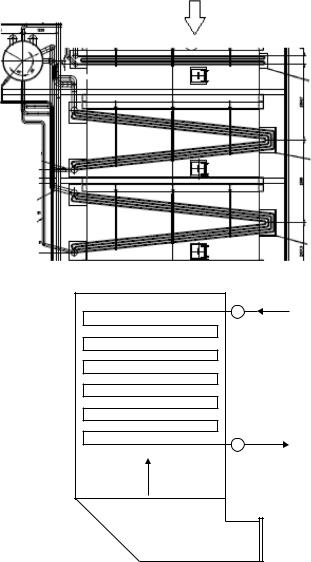
190 |
Steam Generators and Waste Heat Boilers: For Process and Plant Engineers |
Gas in
Drum
(c)
Water in |
Steam out |
Superheater
Evaporator 1
Evaporator 2
(d)
FIGURE 4.21 (Continued)
(c) Inclined evaporator tubes provide more comfort factor. (d) Once-through HRSG.
OTSGs can be started up and shut down quickly due to the low mass of water and steel (water equivalent). On the flip side, the steam pressure decay is faster when the gas turbine trips than in designs having a steam drum and large water inventory. Absence of downcomer and riser piping makes the layout easier and lowers their cost of fabrication and erection. The two-phase pressure drop inside the tubes could be large and could be in the range of 8–12 bar depending on steam pressure and a significant operating cost.
The once-through steam generator (see Chapter 3) used in steam flooding applications generates 80% quality steam at high steam pressures using the energy from gas turbine exhaust as well. These units generate steam at 100–200 barg depending on the depth of oil
Waste Heat Boilers |
191 |
field. Multiple streams are used in large HRSGs with flow control valve at the water inlet of each stream to ensure that two-phase instability problems with water–steam mixture do not arise. Eighty percent quality steam may also be generated using exhaust gases from gas turbines. The HRSG is also designed to ensure low heat flux inside the tubes by manipulating the fin geometry. Since many HRSGs use horizontal tubes, the allowable heat flux is limited to 270,000 kcal/m2 h (100,000 Btu/ft2 h or 314 kW/m2). The wet steam (80% quality) ensures that the salts in feed water such as sodium are soluble in the steam– water mixture and are not deposited inside the tubes and carried away with the steam– water mixture. To minimize acid or water dew point concerns, a heat exchanger to preheat the cold water is used as shown.
Figure 4.22a shows a plant with furnace-fired HRSGs, while Figure 4.22b shows the details of its construction. As discussed earlier, the convection sections follow the furnace, and finned tubes of varying density are used in the convection section to keep the tube wall and fin tip temperatures low. Downcomers are located at the rear as shown. The convection bank is followed by an economizer. Figure 4.22c shows a dual-pressure natural circulation HRSG in the field.
Another interesting application in gas turbine plants is the intercooler for compressed air used for combustion (Figure 4.23). Intercooling improves the efficiency of compression process in gas turbine compressors. Hot compressed air from the first stage of the compressor is cooled by feed water (typically high-pressure economizer water) before it is again sent back to the next stage of the gas turbine compressor and combustor. Since the air is at high pressure and the water also is at high pressures, say, 100–150 barg, the heat transfer coil should be placed inside a pressure vessel with high-pressure–high-temperature air, typically at 15–25 barg and at 400°C–450°C outside the tubes and the colder water inside the tubes in counter-flow direction. Finned tubes are used for the coil. Baffles are used to divert the pressurized air over the finned tube bundle and then exit the pressure vessel.
Fluid heaters are another important application of turbine exhaust. Industrial heat transfer fluids such as therminol, glycol, or even hot water are heated by turbine exhaust. A finned coil is used in these applications. The coil looks like an economizer. As many of these fluids have limitation on heat flux and have a low tube-side heat transfer coefficient (compared to water), low fin density not exceeding 98–117 fins/m should be used on the heating surfaces.
Natural versus Forced Circulation HRSGs
In the United States, the trend is to use natural circulation HRSGs, while in Europe, the forced circulation units are the norm. Some thoughts on these designs are outlined in the following text:
1.Natural circulation units do not require a pump for maintaining circulation through the evaporator tubes. Static head available, steam pressure, and system resistance caused by size and length of downcomer, riser pipes determine the CR. The use of circulation pumps in forced circulation units involves an operational and maintenance cost, and their failure for some reason such as power outage or pump failure could shut down the HRSG.
2.The water boils inside vertical tubes in natural circulation units, and the steam bubbles move upward, which is the natural path for them; hence, the tube walls are completely wetted by water (if heat flux is nominal). With horizontal tubes, there is a difference in temperature between the top and bottom portions of the

192 |
Steam Generators and Waste Heat Boilers: For Process and Plant Engineers |
(a)
|
Furnace |
|
|
|
Screen |
Evaporator |
|
Burner |
Superheater |
||
|
|||
(b) |
|
||
|
|
(c)
FIGURE 4.22
(a) Furnace-fired HRSGs in operation. (b) Furnace-fired HRSG plan view. (c) Dual-pressure natural circulation HRSG. (Courtesy of Cleaver Brooks, Thomasville, GA.)

Waste Heat Boilers |
193 |
Air out
Water in
Water out
Air in
FIGURE 4.23
Pressurized hot air water preheater. (Courtesy of Cleaver Brooks, Thomasville, GA.)
tubes, which could cause thermal fatigue. Also if the selection of streams is not proper and if the velocity of the steam–water mixture is not high enough, the vapor phase can separate from liquid phase leading to steam blanketing and possibly overheating of tubes. This is a possibility when the HRSG is fired and the heat flux inside the tubes is high, particularly when high fin density is used and also if the gas temperature profile at the tube bundle is nonuniform.
3.Natural circulation system with vertical tubes can tolerate higher heat flux generally 50%–80% more than horizontal tube designs. If there is a nonuniformity in gas temperature or heat flux at any cross section, the tube receiving the higher heat flux will have a higher CR due to the greater differential in fluid densities between the more dense fluid in the downcomer circuit and the less dense mixture in the evaporator tubes, which is helpful to even out the imbalances. In forced circulation units, the flow resistance of all tubes is nearly the same as well as the flow of mixture and any severe variation in gas flow and temperature at a cross section can cause some tubes to generate more steam and hence be vulnerable to tube failures.
4.Natural circulation units require more real estate than forced circulation units. The floor space can run into several hundred feet if there are multiple modules
and catalysts for NOx, CO control. In forced circulation units, the floor space may be small, but the height of the HRSG will be large requiring more support steel, ladders, and platforms.
5.The horizontal gas flow configuration of natural circulation units provides an easy way for water washing the highly soluble ammonia compounds formed downstream of the selective catalytic reduction (SCR) when operating with a sulfur-containing fuel. When a vertical gas flow unit is water washed, the slush and corrosive products are likely to deposit over the SCR below the low-temperature surfaces.

194 |
Steam Generators and Waste Heat Boilers: For Process and Plant Engineers |
6.The economizer water flows downward in a forced circulation unit with gas flowing from bottom to top. Hence, if steam bubbles are formed at low loads, there is a possibility of flow stagnation inside tubes. One way to overcome this is to place the feed water control valve between the economizer and the evaporator so that the operating pressure of the economizer is increased and some approach temperature (difference between saturation temperature at that pressure and water exit temperature) is available.
7.The casing of the forced circulation unit is typically hot as it is easier to contain the tube bundles inside the casing and support them. However, this requires external insulation, and the hot casing requires alloy steel depending on gas temperatures. Thermal expansion issues between casing and tube bundles also have to be reviewed.
Emission Control in HRSGs
Chapter 1 shows how one may convert CO and NOx emissions from mass to volumetric basis and how to correct them for 15% oxygen dry. If the desired CO and NOx levels are very low, an SCR system is required. Since these operate efficiently only within a range of gas temperatures typically 350°C–420°C (Figure 4.24), the HRSG should be designed suitably that in unfired as well as in fired modes or at part load operation of the gas turbine, the range of gas temperatures at the SCR can be satisfied. The ammonia grid (Figure 4.25) must be located such that the ammonia injected into the gas stream mixes well with exhaust gas. The use of catalysts affects the HRSG design and performance in a few ways. The gas pressure drop across the CO or NOx catalyst can be on the order of 25–40 mm wc including the duct work to match the HRSG cross section with that of the catalyst. The evaporator in almost all cases has to be split up into two parts as shown in Figure 4.26 so that the NOx catalyst can be located in between the two evaporators; the sizing of the evaporators have to be checked at all loads to ensure that the window of gas temperature is obtained at all loads. Figure 4.27 shows how the gas temperature varies at each heating surface as a function of gas inlet temperature. These two evaporators will operate in parallel and are connected to the common steam drum with external downcomers and risers. The lengths of these pipes can be significant and run into, say, 20–40 m depending on HRSG height and location of the two evaporators;
Relative activity
100 |
|
|
Typical catalyst activity |
|
|
|
|
|
|||
|
|
|
|
|
|
||||||
98 |
|
|
|
|
|
|
|
||||
96 |
|
|
|
|
|
|
|
|
|
|
|
94 |
|
|
|
|
|
|
|
|
|
|
|
92 |
|
|
|
|
|
|
|
|
|
|
|
90 |
|
|
|
|
|
|
|
|
|
|
|
88 |
|
|
|
|
|
|
|
|
|
|
|
86 |
|
|
|
|
|
|
|
|
|
|
|
84 |
|
|
|
|
|
|
|
|
|
|
|
82 |
|
|
|
|
|
|
|
|
|
|
|
80 |
|
|
|
|
|
|
|
|
|
|
|
500 |
550 |
600 |
650 |
700 |
750 |
800 |
850 |
900 |
|||
Temperature, °F
FIGURE 4.24
Operating temperatures of catalysts.

Waste Heat Boilers |
195 |
FIGURE 4.25
Ammonia grid. (Courtesy of Nebraska Boiler, Division of Cleaver Brooks. Thomasville, GA.)
Steam out
GT exhaust |
Superheater |
|
|
|
|
|
|
Water in |
Stack |
Co catalyst |
AIG |
Boiler evaporator 1 |
SCR |
Boiler evaporator 2 |
Economizer |
|
Ammonia–air mixture
FIGURE 4.26
Arrangement of an HRSG with SCR and CO catalyst.
hence, circulation calculations have to be performed to ensure that the evaporators function well in all modes of operation.
Flow-Accelerated Corrosion
Many utilities and cogeneration plants are finding that flow-accelerated corrosion (FAC) is causing waste age of materials, downtime, and additional maintenance concerns. FAC is defined as the localized rapid metal loss resulting in tube wall thinning of carbon and low

196 |
Steam Generators and Waste Heat Boilers: For Process and Plant Engineers |
|
4 |
|
|
|
|
|
1300 |
|
|
|
|
|
3 |
|
Sh. Evap. SCR |
Evap. Eco. |
|
|
1100 |
|
|
||
|
|
1—Unfired 110,000 Ib/h at 725 F, 600 psig |
|||
°F |
2 |
|
2—Fired |
150,000 Ib/h at 782 F, 600 psig |
|
Temperature, |
|
|
3—Fired |
200,000 Ib/h at 800 F, 600 psig |
|
900 |
|
4—Fired |
250,000 Ib/h at 800 F, 600 psig |
||
1 |
|
|
|
|
|
700 |
|
|
|
|
|
|
|
|
|
|
|
|
500 |
|
|
|
|
|
300 |
Evap. 1 |
Evap. 2 |
Econ. |
Stack |
|
Sh. |
||||
FIGURE 4.27
HRSG gas temperature profiles at various gas inlet conditions.
|
100 |
|
|
|
|
|
|
|
|
|
|
|
|
|
|
|
|
|
|
|
|
|
90 |
|
|
|
|
|
|
|
|
|
ppb |
80 |
|
|
|
|
pH = 8.75 |
|
|
|
|
70 |
|
|
|
|
|
|
|
|
||
dissolution, |
|
|
|
|
|
|
|
|
|
|
60 |
|
|
|
|
|
|
|
|
|
|
|
|
|
|
|
|
|
|
|
|
|
|
50 |
|
|
|
|
|
|
|
|
|
Magnetite |
40 |
|
|
|
|
|
|
|
|
|
20 |
|
|
|
|
9.05 |
|
|
|
|
|
|
30 |
|
|
|
|
|
|
|
|
|
|
10 |
|
|
|
9.6 |
|
|
|
|
|
|
0 |
|
|
|
|
|
|
|
|
|
|
|
|
|
|
|
|
|
|
|
|
|
50 |
100 |
150 |
200 |
250 |
300 |
350 |
|||
Temperature, °C
FIGURE 4.28
FAC as a function of temperature and pH of water.
alloy piping. FAC is known to occur in the region of 125°C–220°C as shown in Figure 4.28. In HRSGs, the evaporators and economizers in the LP (low pressure) and IP (Intermediate pressure) sections are affected. FAC is the absence of protective metal oxide layer that when present limits corrosion in boiler systems. Without this protection, the surface is free to react with the passing water (or two-phase flow), and metal loss is rapid. Factors affecting FAC are flow velocity, geometry, metallurgy, dissolved oxygen concentration, and temperature. Feeder connections with sharp bends are common in HRSGs. These multiple feeders connect the downcomer pipes to the evaporator circuits and take the steam–water mixture to the drum.
Past industry practices believed that all of dissolved oxygen must be eliminated from feed water to control corrosion. To deoxygenate the feed water, oxygen was mechanically
Waste Heat Boilers |
197 |
removed in the condenser–deaerator system with an addition of an oxygen scavenger such as hydrazine to maintain a residual of 40–100 ppb hydrazine. This caused the feed water to become more and more reducing and has produced the opposite effect of producing a protective layer. The normally protective magnetite layer in carbon and low alloy steel dissolves into a stream of flowing water or two-phase flow. Both the pH and temperature and level of dissolved oxygen influence the stability and solubility of the magnetite oxide layer. The difference in wall loss due to FAC is 100 times greater at 1 ppb dissolved oxygen in feed water than at 20 ppb. Hence, maintaining some residual oxygen will reduce the FAC.
In Germany, the maximum oxygen in feed water has been increased from 0.02 to 0.1 (20–100 ppb) mg/kg. Flow velocity is also lowered to reduce the erosion of the magnetite layer. HRSGs have sharp bends in economizers, evaporators that are prone to FAC. FAC also develops at flow disturbances such as elbows, bends, reducers, tees, and steam attemperating lines. Sometimes the bends are made of low chromium alloys to reduce FAC. In oxygenated treatment, oxygen is deliberately introduced in the condensate and feed water system. PH of feed water is raised to 9.2–9.6 for FAC effect to be minimal by an addition of ammonia. It has been found that two-phase FAC is difficult to control chemically and hence 1.25 chromium steels are suggested for such areas. All volatile treatment used in some boiler including once-through units to avoid deposition of solids leads to the dissolution of the protective magnetite.
Water Tube Waste Heat Boilers: Sizing and Performance
Before proceeding with the examples on water tube boiler and fire tube boiler performance, one should review Appendices A through F. Design and off-design calculations, and estimation of heat transfer coefficients inside and outside plain and finned tubes are discussed. Simplified approach to estimating tube-side heat transfer coefficient for several fluids is also explained. With this background, it should be easy to apply the concepts to real-life design issues on both fire tube and water tube boilers.
Optimizing Pinch and Approach Points in HRSGs
Chapter 5 explains the importance of pinch and approach points and how they are selected. Procedure to estimate the steam generation and gas–steam temperature profiles is also discussed. When trying to maximize steam generation, HRSG suppliers should use the lowest pinch and approach points avoiding the possibility of steaming at low loads; cost is also a factor. Plant engineers should also be able to evaluate proposals with different pinch and approach points and choose the best offering. Presented in the following text is an example of HRSG proposal from two different vendors.
Example 4.1
A gas turbine of capacity 7.5 MW has an exhaust gas flow of 100,000 kg/h at 500°C. Gas analysis is % volume CO2 = 3, H2O = 7, N2 = 75, and O2 = 15. In the unfired mode, the HRSG will generate about 15,000 kg/h, while 40,000 kg/h of saturated steam at 40 kg/cm2 g is required by the plant, which will be achieved by supplementary firing; the HRSG is likely to operate 50% of the time in unfired mode and 50% of the time in fired mode. The boiler performance in various cases is shown later. Vendor A has

198 |
Steam Generators and Waste Heat Boilers: For Process and Plant Engineers |
TABLE 4.6
HRSG Designs with Low and High Pinch Points
|
|
Vendor A |
|
Vendor B |
||
|
|
|
|
|
|
|
Data Case |
|
Unfired Mode |
Fired Mode |
|
Unfired Mode |
Fired Mode |
|
|
|
|
|
|
|
Gas flow, kg/h |
100,000 |
100,000 |
100,000 |
100,000 |
||
Gas temp. in, °C |
500 |
500 |
500 |
500 |
||
Firing temperature, °C |
500 |
925 |
500 |
952 |
||
Gas temp. to eco, °C |
256 |
264 |
271 |
302 |
||
Stack gas temp., °C |
168 |
133 |
190 |
168 |
||
Gas press. drop, mm wc |
159 |
176 |
107 |
121 |
||
Feed water in, °C |
105 |
105 |
105 |
105 |
||
Water to eco, °C |
242 |
189 |
241 |
192 |
||
Sat temperature, °C |
251 |
251 |
251 |
251 |
||
Burner duty, MM kcal/h |
0 |
13.0 |
0 |
14.0 |
||
Steam flow, kg/h |
15,565 |
40,000 |
14,587 |
40,000 |
||
Evaporator surface, m2 |
2,951 |
|
1,908 |
|
||
Economizer surface, m2 |
2,129 |
|
1,296 |
|
||
Boiler duty, MM kcal/h |
8.75 |
22.51 |
8.21 |
22.51 |
||
Pinch point, °C |
5 |
13 |
20 |
51 |
||
Approach point, °C |
9 |
62 |
10 |
59 |
||
No of rows deep, evap. |
21 |
|
15 |
|
||
No of rows deep, econ. |
14 |
|
8 |
|
||
Efficiency, % |
68.8 |
87.5 |
64.6 |
84.2 |
||
Note: 50.8 × 44 mm tubes, 24 tubes/row, length of evaporator = 4 m, length of economizer tubes = 3.5 m. staggered arrangement, 101.8 mm pitch, 197 × 19 × 1.5 solid fins. Burner duty is on fuel lower heating value basis.
provided a bigger boiler with a lower pinch point, while vendor B has offered a smaller boiler that requires more fuel than vendor A to generate the same amount of steam. The plant engineer has to evaluate which offering is better (Table 4.6).
Let us use the following cost factors for evaluating the better option; cost of steam: $10/1000 kg; cost of electricity = 11 cents/kWh; cost of fuel = $1/MM kcal/h.
Vendor A has used a lower pinch point and has a bigger evaporator and economizer.
1.Advantage of A over B in steam generation in unfired mode = (15,565 − 14,587) × 4,000 × 10/1,000 = $39,120.
2.Advantage of A over B in fired mode: (14 − 13) × 1 × 4000 = $16,000.
3.Typically, 100 mm wc back pressure increase in the HRSG is equivalent to 1% loss in gas turbine power output. Hence, advantage of B over A is (−107 − 121 + 159 + 176) = 107 or an average of 53.5 mm wc throughout the year = 7,500 × 0.01 × 0.11 × 8,000 × 53.5/100 = $35,310.
Hence, annual savings of design A over design B = 39,120 + 16,000 − 35,310 = $19,810. One may check the difference in price and compute the payback period for vendor A.
It is likely that vendor A is a better option though the initial cost may be slightly more. The payback may not be that long, considering that the cost of instruments, controls, casing, duct, and supporting steel may not be that much different and only the HRSG per se may differ in cost. The purpose of the exercise is to show how to evaluate the variables affecting the operating costs and see if a higher investment in lower pinch point is worth the money.
Waste Heat Boilers |
199 |
HRSG Performance and Evaluating Field Data
When a new waste heat boiler is installed, its operating data may differ from that stated in the proposal. There can be several reasons for this such as the following:
•The inlet flue gas flow and temperature may be different from that used in the proposal or guarantee statement. An unfired waste heat boiler simply responds to the inlet gas conditions, and hence, the steam parameters may be different from those expected.
•The plant’s operating feed water temperature or pressure may be slightly different from that used for generating the proposal due to plant’s limitation, deaerator or water treatment plant’s availability. Hence, steam generated or exit gas temperature from boiler may differ from that stated in the proposal.
The question then arises: how can the plant engineer ensure that the boiler has been sized correctly, and will it generate steam at the rated conditions when provided with the rated gas flow and temperature?
Let us consider an unfired HRSG as shown in Figure 4.21a. It was noticed that the operating data were completely different from that predicted by the HRSG supplier. As discussed earlier, one has to investigate the reasons for this. It is likely that the gas turbine is operating at a different load or ambient temperature resulting in variations in exhaust gas flow and temperature from that used for guarantee purposes; the plant may not be able to operate the gas turbine at guarantee load conditions; also, portion of the exhaust gas may have been bypassed as steam demand may not be there during the testing phase and plant does not wish to waste the treated water. While testing a boiler, plant engineers typically shut off the blowdown line and ensure dampers and valves do not leak.
Then the question arises: are the differences between operating data and guaranteed data reconcilable or out of line and whether the HRSG itself was designed properly? If the performance test is not carried out within a few months of installation and if the plant cannot operate the HRSG at the rated conditions, it may not be able to find out if the HRSG was designed correctly or not. The HRSG supplier can blame the plant for not providing proper conditions for testing the HRSG and can walk out without proving if the HRSG design was adequate or not. This is not good from the plant’s perspective. The bottom line is how to check if the HRSG was properly sized or not even if the HRSG operates at different parameters from those guaranteed. The following example shows how one can evaluate the performance of an operating HRSG. The procedure may be used for any waste heat boiler. Figure 4.29 shows the logic or flow diagram for off-design performance calculations of waste heat boilers. There are several iterations, and for each change in gas temperature or steam temperatures, the properties have to be evaluated at each component. If there are multiple modules or if the HRSG is fired, the calculations become more tedious.
Example 4.2
An unfired gas turbine HRSG has the data shown in Table 4.7. The design shows over 15.3 t/h of steam at 463°C at 40 kg/cm2 g with 105°C feed water. However, in operation, it makes only 11,000 kg/h at 442°C and at 35 kg/cm2 g with feed water at 120°C with zero blowdown. The water temperature leaving the economizer is measured as 242°C. The plant is not able to operate at 40 kg/cm2 g with feed water at 105°C for various other reasons. Inlet and exit gas temperatures are measured as 500°C and 190°C. Is this performance acceptable? The HRSG supplier says that due to variations in exhaust gas flow and temperature, they are not able to get the desired steam flow of 15.3 t/h at 460°C and that his HRSG design is perfect.

200 |
Steam Generators and Waste Heat Boilers: For Process and Plant Engineers |
|||
|
Start |
tg1 |
tg2 |
|
|
ts2 |
|
tg3 |
|
|
|
|
||
|
|
|
|
|
Input Wg, tg1, gas, analysis, steam |
|
ts |
tg4 |
|
|
pressure, tw1, A1, A2, A3 |
|
|
tw2 |
|
Assume Ws |
|
|
tw1 |
|
|
|
|
|
Assume ts2 |
|
Assume tw2 |
Compute Qa |
|
|
Compute tg2 |
|
compute Qa, tg4 |
Compute Qt |
|
compute Qt |
Q1 = Qt |
|
No |
No |
|
|
(Qa–Qt)/Qa |
|
(Qa–Qt)/Qa |
<0.01 |
|
<0.01 |
|
|
Yes |
Yes |
|
Q3 = Qt |
Compute Q2, tg3 |
|
Compute Wc using |
|
|
Q1, Q2, Q3, ts2 |
Wc = Ws |
No |
(Ws–Wc)/Ws |
|
|
|
|
|
<0.01 |
|
|
Yes |
|
|
End |
Wg
Sh. Evap. Eco.
Notes: Un„red performance, NTU method used for solving all surfaces
A1, A2, A3=surface areas of superheater, evaporator, Economizer
Wg, Ws = gas, steam Šows
Q1, Q2, Q3=duty of superheater, Evaporator and economizer
FIGURE 4.29
Logic diagram for HRSG performance evaluation.
TABLE 4.7
Gas Turbine HRSG Tube Geometry Data
Geometry |
Sh. |
|
|
Tube OD |
31.8 |
Tube ID |
26 |
Fins/in. or fins/m |
78 |
Fin height |
19 |
Fin thickness |
1.9 |
Fin width |
4 |
Fin conductivity |
35 |
Tubes/row |
20 |
Number of rows deep |
6 |
Length |
4 |
Transverse pitch |
84 |
Longitudinal pitch |
101 |
Streams |
20 |
Evap. Econ.
50.831.8
44 |
26 |
197 |
197 |
19 |
19 |
1.91.9
4 |
4 |
35 |
35 |
20 |
20 |
18 |
14 |
4 |
4 |
101 |
84 |
101 |
100 |
0 |
10 |
Note: Streams are the number of tubes carrying the steam or water. This is explained in Appendix B.

Waste Heat Boilers |
201 |
This type of situation often arises in plants operating HRSGs. The HRSG in all likelihood will operate at parameters slightly different from those stated in the proposal document. Hence, the steam output and the gas–steam temperature profiles will be different from the proposal data. If questioned, the HRSG supplier will cite the gas turbine exhaust conditions for the field performance results, and the gas turbine supplier will suggest that the plant look into the HRSG design. The helpless plant engineer will be better off if he knows how to evaluate the performance himself and get an idea of what is going on.
Tube geometry data is shown in Table 4.7; thermal performance data as shown in Table 4.8 should be obtained from HRSG suppliers for each operating case such as full load and part load of gas turbine and at a few different ambient temperatures, before the HRSG is ordered! If it is a multiple-pressure unit, then such geometric and thermal performance data should be provided for each component in the highand low-pressure sections. Without a clear performance and geometric data, one cannot evaluate the performance of the HRSG independently. Even if the U values are not given by the HRSG supplier, using the basic equation Q = UAΔT, one may compute the ΔT (from the gas, steam temperature data), and based on surface area and duty shown, compute the U value. Then one may adjust the U value for gas temperature and gas flow variations as follows (this method of adjusting the U value for off-design conditions is also discussed in Chapter 5 on simulation):
|
Wf 0.65 |
|
Fgf |
|
||
Uf = Ud |
|
|
|
|
|
(4.1) |
|
|
|||||
Wd |
|
|
|
|
||
|
Fgd |
|
||||
where Fg is a factor depending on gas properties = (Cp0.33k0.67/µ0.32).
Subscripts f and d refer to field and design conditions. Gas properties are computed at the average gas temperature of each section as finned tubes are typically used. W refers to gas flow in mass units.
TABLE 4.8
HRSG Performance Data
|
Gas Flow = 110,000 kg/h |
||
|
Design Case |
|
|
|
|
|
|
Process Data Surface |
Suphtr. |
Evap. |
Econ. |
|
|
|
|
Gas temp. in, ±5°C |
550 |
482 |
265 |
Gas temp. out, ±5°C |
482 |
265 |
183 |
Gas spht., kcal/kg °C |
0.2756 |
0.2691 |
0.2596 |
U, kcal/m2 h °C |
52.39 |
30.96 |
39.11 |
LMTD, °F |
147 |
75 |
42 |
Duty, MM kcal/h |
2.06 |
6.34 |
2.33 |
Surface area, m2 |
268 |
2749 |
1407 |
Gas press. drop, mm wc |
16.53 |
87.42 |
41.82 |
Foul factor, gas |
0.0004 |
0.0004 |
0.0004 |
Steam Side |
|
|
|
Steam pres, kg/cm2a |
41 |
42 |
42 |
Steam flow, kg/h |
15,313 |
15,313 |
15,773 |
Fluid temp. in, °C |
253 |
245 |
105 |
Fluid temp. out, ±5°C |
463 |
253 |
245 |
Press. drop, kg/cm2 |
1.5 |
0.0 |
0.6 |
Foul factor, fluid |
0.0002 |
0.0002 |
0.0002 |
Spray, kg/h |
0 |
|
|
Gas analysis: % volume CO2 = 3, H2O = 7, N2 = 75, O2 = 15.
202 |
Steam Generators and Waste Heat Boilers: For Process and Plant Engineers |
If U is not provided, the duty Q and the temperature profiles will be known from which ΔT and U may be estimated for each section such as superheater, evaporator, and economizer. Let us assume that the customer has provided them as shown in Tables 4.7 and 4.8 in our case. One may also use the method discussed in Appendix E for finned tubes and evaluate U for each section and check the values provided by the HRSG supplier. They also should be aware of the fact that fin geometry influences U significantly.
Let us estimate the exhaust gas flow from the inlet and exit gas temperatures and the steam parameters, which are presumed to be more accurately measured than the gas flow. The total energy absorbed by steam = 11,000 × (792.4 − 120.9) = 7.38 × 10⁶ kcal/h (792.4 and 120.9 kcal/kg refer to the enthalpy of superheated steam and feed water, and blowdown was neglected). Gas specific heat at average gas temperature of (500 + 190)/2 = 345°C is 0.266 from Table F.6. Hence, exhaust gas flow = 7,380,000/[0.266 × (500 − 190)× 0.99] = 90,400 kg/h (0.99 refers to casing heat loss of 1%). As discussed in Chapter 6, one may estimate the casing heat loss based on provided insulation thickness; however, for this exercise, 1% heat loss is a good assumption.
Since some variations in exhaust gas temperature profile are present, one may apply correction factor Fg while estimating U from the design data. (The accurate method is to develop a program that estimates U using the detailed procedure discussed in Appendix E on finned tubes after computing the inside and outside heat transfer coefficients and fouling factors.) Fg at average gas temperature of 366°C in design case is 0.4143 and at operating case is 0.4112. Hence, a correction of (0.4112/0.4143) = 0.992 may be applied to U; however, for this exercise, we are not applying temperature correction factor as the main purpose is to show how much steam the HRSG should be making and see if the field data are reasonable. Since the steam flow is significantly lower, the superheater, U, may be reduced by a factor (11,000/15,300)0.15 = 0.952 (see Chapter 5 or Ref. [1]).
For superheater, U = 52.39 × 0.952 × (90,400/110,000)0.65 = 43.9 kcal/m2 h °C
For evaporator, U = 30.96 × (90,400/110,000)0.65 = 27.25 kcal/m2 h °C
For economizer, U = 39.11 × (90,400/110,000)0.65 = 34.43 kcal/m2 h °C
Superheater Performance
One may refer to the NTU method discussed in Appendix A. The specific heat of steam between 442°C and saturation of 245°C is (792.4 − 669.3)/(443 − 245) = 0.622 kcal/kg °C (specific heat is enthalpy difference divided by temperature difference). The specific heat of exhaust gas may be taken as 0.273 in the superheater based on the exhaust gas analysis and data in Appendix F on gas properties (and can be checked in the second iteration). Cmax = 90,400 × 0.99 × 0.273 = 24,432. Cmin = 11,000 × 0.622 = 6,853.
|
|
C = |
Cmin |
= |
|
6853 |
|
= 0.28.(1 − C) = 0.72 |
|
|
|
|
|||||||||
|
|
24432 |
|
|
|
|
|
||||||||||||||
|
|
|
Cmax |
|
|
|
|
|
|
|
|
|
|
|
|
||||||
|
|
NTU = |
|
|
UA |
= 268 × 43.9 = 1.717 |
|
|
|
|
|
||||||||||
|
|
|
|
|
|
|
|
|
|
||||||||||||
|
|
|
|
|
Cmin |
6853 |
|
|
|
|
|
|
|
|
|||||||
|
1 − exp{−NTU × (1 |
− C)} |
|
|
{1 − exp(−1.717 × 0.72)} |
|
|
||||||||||||||
= |
|
|
|
|
|
|
|
|
|
= |
|
− |
|
× |
|
(− |
× |
|
) |
|
|
1 − C exp{−NTU |
× (1 − C)} |
|
|
|
|
|
|||||||||||||||
|
|
|
|
|
|
|
|
|
|
|
(1 |
|
0.28 |
|
exp |
1.717 |
|
0.72 |
|
) |
|
= |
0.7095 |
= 0.772. |
|
|
|
|
|
|
|
|
|
|
|
|
|
|
|
|
|
|
|
0.9187 |
|
|
|
|
|
|
|
|
|
|
|
|
|
|
|
|
|
|
|||
|
|
|
|
|
|
|
|
|
|
|
|
|
|
|
|
|
|
|
|
|
|
The Q = 0.772 × 6823 × (500 − 245) = 1.349 × 10⁶ kcal/h
Waste Heat Boilers |
203 |
Exit gas temperature of superheater = 1,349,000/90,400/0.99/0.273 = 444°C.
Exit steam temperature = 245 + (1,349,000/6,823) = 442°C
Evaporator Performance
See Appendix A for evaporator performance evaluation.
Using the equation Ln (tg1 − ts)/(tg2 − ts ) = UA/(WgCpg 0.99)
|
(444 − 245) |
|
27.25 |
× 2749 |
|
|
|||
Ln |
|
|
|
= |
|
|
|
= 3.12 or tg2 |
= 254°C |
(tg2 |
|
(90400 × .99 |
× 0.268) |
||||||
|
− 245) |
|
|
|
|||||
|
|
|
|
|
|
|
|
|
|
Q = 90,400 × 0.99 × (444 − 254)× 0.268 = 4.56 × 10⁶ kcal/h
Economizer Performance
C = 11,000 × 1.05655/(90,400 × 0.99 × 0.258) = 0.503 (specific heat of water and gas may be shown to be 1.05655 and 0.258). (1 − C) = 1 − 0.503 = 0.497. Cmin = 11,000 × 1.05655 = 11,622.
|
|
NTU |
34.43 × 1407 |
= 4.168 |
|
|||
|
|
= |
|
|
||||
|
|
(11000 × 1.05655) |
||||||
|
|
1 − exp(−4.168 × 0.497) |
0.874 |
|
||||
= |
|
|
|
|
= |
|
= 0.933 |
|
1 |
− 0.503 |
× exp(−4.168 × 0.497) |
0.9366 |
|||||
|
|
|
|
|
|
|
|
|
Q = 0.933 × 11622 × (254 − 120) = 1.453 × 10⁶ kcal/h
Exit gas temperature = 254 − 1,4540,000/(90,400 × 0.99 × 0.258) = 191°C (agrees with the measured value)
Exit water temperature = 120 + 14,530,000/(11000 × 1.05655) = 245° C (cclose to steaming)
Total duty transferred = 1.349 + 4.56 + 1.453 = 7.36 MM kcal/h (close to that from field data). Hence, the performance at part load is what can be reasonably expected from the revised gas conditions. Hence, the HRSG may be said to be performing well. One may also in a similar manner review the performance data provided at design conditions and see if 15,300 kg/h of steam at 463°C can be generated under the gas conditions used for performance guarantee. Actual steam generation = 7.36 × 10⁶/(792.4 − 120.9) = 10,960 kg/h agrees with the measured value of 11,000 kg/h.
Hence, the HRSG performance is satisfactory. If the exit gas temperature had been 210°C or the steam generation was, say, 10,300 kg/h, then one may have to investigate further the sizing of the HRSG. Hence, even though the steam parameters such as pressure and feed water temperature have changed slightly, it has been shown by process calculations that the HRSG performance is reasonable. This is a simple and quick estimate. Plant engineers may develop calculation modules correcting for gas and steam properties and generate more accurate numbers.
One can estimate the gas pressure drop also and compare it with the measured value. Calculations with supplementary-fired HRSGs are more involved, as discussed in Chapter 1, but following the same procedure and a few more rounds of iterations, one can
204 |
Steam Generators and Waste Heat Boilers: For Process and Plant Engineers |
evaluate the performance from field data. One may also work from the economizer end and proceed toward the superheater and check the inlet gas temperature.
Efficiency of Waste Heat Boiler, HRSG
The efficiency E of a waste heat boiler is obtained as follows:
E = (energy absorbed by steam and water or other fluids)/(exhaust gas flow × enthalpy at entering temperature + fuel input if any on LHV basis)
In Example 4.2, the energy absorbed by steam–water in the superheater, evaporator, and economizer of the HRSG = 10.73 MM kcal/h; exhaust gas flow = 110,000 kg/h at 550°C. Exhaust gas analysis is % volume CO2 = 3, H2O = 7, N2 = 75, and O2 = 15. The efficiency E = 10.73 × 10⁶/(110,000 × 140.8) = 0.68 or 69%. (Enthalpy of 140.8 kcal/kg was estimated from Table F.12 for the unfired turbine exhaust gas at 550°C.)
In the example shown in Table 4.6, the efficiency in unfired case in column 1: E = 8.75 × 10⁶/(100,000 × 127.1) = 68.8%. In the fired case, column 2, E = 22.51 × 10⁶/(100,000 × 127.1 + 13 × 106) = 87.5%.
Advantages of Supplementary Firing in HRSGs
As discussed in Chapter 1, there is lot of oxygen in turbine exhaust gases that can be utilized to fire additional fuel to the exhaust gas and thus increase its temperature. Increase in inlet gas temperature generates additional steam in the evaporator, which increases the capacity of the heat sink, which is the economizer. Hence, the exit gas temperature beyond the economizer will be lower in the fired mode compared to the unfired mode. Since additional air is also not added, the lower exit gas temperature helps to increase the fuel utilization significantly. It can be shown through performance calculations that supplementary firing is an excellent way of generating additional steam in HRSGs and fuel utilization is nearly 100% or even more. That is, one can generate additional steam with nearly the same amount or lesser amount of fuel. In conventional steam generators, the LHV efficiency is about 93%, while in HRSGs, it can be close to 100% or even more. A layman’s explanation for this is as follows: when we increase excess air in steam generators, the efficiency decreases. In gas turbine HRSGs, we decrease the excess air by firing fuel into the oxygen-rich exhaust gas and hence efficiency is higher. In addition, the exit gas temperature from the economizer exit is lower when inlet gas temperature is higher and that contributes to the higher efficiency as well. The economizer acts as a larger heat sink in the fired mode due to the larger flow of water through it and hence is able to cool the exhaust gases to a lower temperature. Chapter 5 on simulation gives examples of improved fuel utilization with supplementary firing.
In Example 4.1, one may check the fuel utilization also. The difference in energy recovered between the unfired and fired cases for vendor A is (22.51 − 8.71) = 13.80 MM kcal/h, while only 13.0 MM kcal/h is fired on LHV basis. That means the fired case is more than 100% efficient. In the case of steam generators, the efficiency on LHV basis was shown to be about 93.5%. That is, by firing in an HRSG, we straightaway get more than 100% fuel utilization. If we look at vendor B, the additional energy from steam = 22.51 − 8.21 = 14.3 MM kcal/h, while 14.0 MM kcal/h is fired! Here again, it is more than 100% efficient. Thus, plant engineers may analyze the HRSG performance in both fired and unfired cases and understand how well the fuel energy is utilized. (The HRSG should have an economizer to be more efficient in the fired
Waste Heat Boilers |
205 |
mode if it is a single-pressure unit. If we did not have an economizer, the exit gas temperature will be higher without an economizer and hence efficiency in fired mode will be lower.)
Thus, supplementary firing is one way to improve the efficiency of gas turbine HRSGs. That is because we are not adding any combustion air while firing but utilizing the oxygen in the exhaust. In effect, we are reducing the excess air. The heat losses from the boiler are also lowered due to the lower exit gas temperature in the fired case. This is due to the fact that a larger heat sink is available in the form of the economizer in the fired mode with the gas flow remaining the same. Plant engineers while planning future projects with HRSGs in cogeneration plants may consider supplementaryor furnace-fired HRSGs as they are more efficient. Since the cross section of an HRSG is determined by the gas flow, it does not matter whether the steam output is 15 t/h or 60 t/h, as the same exhaust gas flow with different temperatures and analysis flows through the HRSG. The size of drums may be larger for the higher capacity, but the overall cost should not be much more than an unfired unit.
HRSG and Steam Generator Performance
When large amount of steam is required from turbine exhaust, furnace firing is resorted to as discussed earlier. When an HRSG and a steam generator are available in a plant, the plant engineer is faced with the issue of maximizing the steam output with minimum fuel input and how to load each of them in an efficient manner. This is due to the fact that the characteristics of an HRSG and a steam generator versus load are different. Figure 4.30 shows the variations in economizer exit gas temperature, water temperature leaving economizer, and efficiency on LHV basis for both a furnace-fired HRSG and a comparable steam generator. Saturated steam pressure = 30 kg/cm2 g; feed water temperature = 105°C; fuel is natural gas (methane = 97%, ethane = 2%, and propane = 1%). Excess air of 15% is used in the steam generator. For the gas turbine, the exhaust gas flow = 100,000 kg/h at 485°C. Exhaust gas analysis = % volume CO2 = 3, H2O = 7, N2 = 75, and O2 = 15. An O-type boiler as shown in Figure 4.22b is used. This has a furnace section followed by convection bank tubes and an economizer. A furnace is required as the firing temperature is about 1250°C in the 100% fired case. A computer program was used in the evaluation.
Optimum Utilization of Boilers
Once the performance characteristics of steam generators and HRSGs are known, one may use the information to generate steam efficiently.
Example 4.3
The performance curves for an HRSG and steam generator of capacity 60 t/h are shown in Figure 4.30. Tables 4.9 through 4.11 give more information.
Let us say that the plant needs 75 t/h of steam. This can be obtained in many ways assuming the boilers are available and capable of operating at any load.
It may be seen that when the HRSG is operated at its maximum capacity, the total fuel consumption is the least. This is a simplistic model. With more HRSGs and more steam generators in a large plant, there will be more options to generate a given amount of steam, and it is a good idea to investigate the optimum loading of each boiler by doing a similar study. Also when planning cogeneration plant HRSGs, it is better to purchase fired HRSGs as the steam generation will be more efficient as seen earlier.

206 |
Steam Generators and Waste Heat Boilers: For Process and Plant Engineers |
|
220 |
|
|
|
|
|
|
|
|
|
|
|
|
|
|
|
|
|
% |
|
|
|
200 |
|
|
|
|
|
|
|
|
|
°C |
160 |
|
|
|
|
|
|
|
|
|
Temperature, |
|
|
|
|
|
|
|
|
|
|
|
180 |
|
|
|
|
|
|
Two |
|
|
|
140 |
|
|
|
Tgo |
|
|
|
|
|
|
|
|
|
|
|
|
|
|
|
|
|
120 |
|
20 |
25 |
30 |
35 |
40 |
45 |
50 |
55 |
|
15 |
|||||||||
(a) |
|
|
|
|
|
Steam, kg/h |
|
|
|
|
|
170 |
|
|
Steam generator |
|
|
|
|
|
|
|
|
|
|
|
|
|
|
|||
|
|
|
|
|
|
|
|
|
||
|
160 |
|
|
|
|
|
Two |
|
|
|
|
|
|
|
|
|
|
|
|
|
|
°C |
150 |
|
|
|
|
|
|
|
|
|
|
|
|
|
|
|
|
|
|
|
|
Temperature, |
140 |
|
|
|
|
|
% |
|
|
|
|
|
|
|
|
|
|
|
|
||
|
130 |
|
|
|
|
|
|
|
|
|
|
|
|
|
|
Tgo |
|
|
|
|
|
|
120 |
|
|
|
|
|
|
|
|
|
|
110 |
|
|
25 |
|
35 |
|
45 |
|
55 |
|
15 |
|
|
|
|
|||||
(b) |
|
|
|
|
|
Steam, kg/h |
|
|
|
|
FIGURE 4.30
Load versus performance for an HRSG and a steam generator.
|
|
|
95 |
|
|
|
|||
|
|
|
90 |
|
|
|
|
85 |
% |
|
|
|
80 |
efficiency,LHV |
|
|
|
|
|
|
|
|
75 |
|
|
|
|
70 |
|
|
|
|
65 |
|
60 |
|
|||
|
100 |
|
||
|
|
|||
|
99 |
|
||
|
98 |
|
||
|
97 |
% |
||
|
|
|
|
|
|
96 |
efficiency, |
||
|
|
|||
|
95 |
|
||
|
94 |
LHV |
||
|
93 |
|||
|
|
|||
|
92 |
|
||
|
91 |
|
||
|
90 |
|
||
|
|
|||
Combined Cycle Plants and Fired HRSGs
It is generally believed that combined cycle plant efficiencies with fired HRSGs are lower than those with unfired HRSGs. The reason is not the poor performance of the HRSG. In fact, the fired HRSG by itself is more efficient than an unfired HRSG. However, the losses associated with the Rankine cycle, particularly when the steam turbine power is a large fraction of the total power output, distorts the results slightly as shown in the following example (it is worked out in British units as all the data were provided in British units, and the purpose is to illustrate the point regarding efficiency).
Waste Heat Boilers |
207 |
TABLE 4.9
Steam Generator
Steam, kg/h |
15,000 |
30,000 |
45,000 |
60,000 |
|
|
|
|
|
Excess air |
35 |
15 |
15 |
15 |
Duty, MM kcal/h |
8.49 |
16.9 |
25.4 |
33.8 |
water temp. to eco, °C |
105 |
105 |
105 |
105 |
Water temp. lvg. eco, °C |
151 |
151 |
158 |
165 |
LHV efficiency,% |
93.36 |
94.46 |
94.34 |
94.07 |
Exit gas temp., °C |
116 |
119 |
127 |
135 |
Burner fuel, MM kcal/h |
8.68 |
17.78 |
26.92 |
35.93 |
|
|
|
|
|
TABLE 4.10
HRSG Performance
Steam, kg/h |
15,000 |
30,000 |
45,000 |
60,000 |
|
|
|
|
|
Steam temp., °C |
234 |
234 |
234 |
234 |
Feed water temp., °C |
105 |
105 |
105 |
105 |
Temp leaving eco, °C |
229 |
197 |
175 |
162 |
Duty, MM kcal/h |
8.49 |
16.9 |
25.4 |
33.8 |
Pinch point, °C |
5 |
10 |
14 |
17 |
Approach point, °C |
5 |
37 |
59 |
72 |
Exit gas temp, °C |
163 |
134 |
126 |
122 |
Burner fuel, MM kcal/h |
0 |
7.9 |
16.3 |
24.7 |
Firing temp, °C |
485 |
748 |
1005 |
1242 |
Note: Steam pressure = 30 kg/cm2 g, fuel-natural gas.
TABLE 4.11
Combined Operation of Steam Generator and HRSG
Total Steam |
HRSG Steam |
Steam Generator |
HRSG Fuel |
SG Fuel |
Total Fuel |
|
|
|
|
|
|
75,000 |
30,000 |
45,000 |
7.9 |
26.92 |
34.82 |
75,000 |
45,000 |
30,000 |
16.3 |
17.78 |
34.08 |
75,000 |
15,000 |
60,000 |
0 |
35.93 |
35.93 |
75,000 |
60,000 |
15,000 |
24.7 |
8.68 |
33.38 |
75,000 |
37,500 |
37,500 |
12.1 |
22.4 |
34.50 |
|
|
|
|
|
|
Example 4.4
A combined cycle plant uses a single-pressure-fired HRSG. The gas turbine used is LM 5000 at 59°F. The following are the basic data:
Exhaust gas flow = 1,030,000 lb/h at 800°F. Exhaust gas analysis: % volume CO2 = 2.8, H2O = 8.5, N2 = 74.4, O2 = 14.3. Power output = 35 MW. Heat rate = 9649 Btu/kWh.
Steam turbine data: Inlet pressure = 650 psia at 750°F. Exhaust pressure = 1 psia. Efficiency = 80% dropping off by 2%–3% at 40% load.
HRSG data: 230°F feed water, 2% blowdown, 1% heat loss. Steam is generated at 665 psia and 750°F. The HRSG generates 84,400 lb/h in the unfired mode and a maximum of 186,500 when fired to 1200°F. The HRSG performance was simulated using the HRSGS

208 |
Steam Generators and Waste Heat Boilers: For Process and Plant Engineers |
||||||||
|
TABLE 4.12 |
|
|
|
|
|
|
|
|
|
Cogeneration and Combined Cycle Efficiency with Fired HRSG |
|
|
|
|||||
|
|
|
|
|
|
|
|
|
|
|
|
|
Boiler |
Burner |
Turbine |
Cogen |
Combined |
|
|
|
Gas Temp.,°F |
HRSG Exit, °F |
Duty |
Duty |
Power |
Plant η, % |
Cycle η, % |
Steam, lb/h |
|
800 |
435 |
99.8 |
0 |
9.2 |
64.9 |
44.7 |
84,400 |
|
|
900 |
427 |
129.9 |
29.6 |
12.1 |
67.9 |
43.8 |
109.700 |
|
|
1000 |
423 |
160 |
59.1 |
15.3 |
70.4 |
43.2 |
135.200 |
|
|
1100 |
420 |
290.4 |
90.7 |
18.2 |
72.3 |
42.4 |
160,960 |
|
|
1200 |
418 |
221.0 |
121.0 |
21.1 |
74.2 |
41.7 |
186,500 |
|
|
Note: Boiler duty is energy absorbed by steam in MM Btu/h. Burner duty is fuel input to HRSG burner in MM Btu/h on LHV basis.
program (Chapter 5), and results are presented in Table 4.12. The system efficiency in both cogeneration and combined cycle mode is calculated as follows:
Gas turbine fuel input = 35,000 × 9,649 = 337.71 MM Btu/h on LHV basis.
Cogeneration mode efficiency at 900°F = 100 × (35 × 3413 + 129.9)/(337.71 + 29.6) = 67.9%
where 129.9 MM Btu/h is the HRSG output and 29.6 MM Btu/h is the HRSG burner input on LHV basis.
Combined cycle mode efficiency = 100× (35 + 12.1) × 3413/(337.71 + 29.6) = 43.8% where 12.1 is the power from the expansion of steam in the turbine. Table 4.12 shows the results with various firing temperatures. It may be seen that cogeneration plant efficiency improves with firing while that of the combined cycle plant decreases. If you check the additional HRSG fuel versus additional boiler duty, you will again find that the HRSG is more than 100% efficient in generating additional steam.
HRSGs with Split Superheaters
When plants do not have demineralized water or if they prefer to tolerate a modest variation in steam temperature between unfired and fired cases, one interesting option is to split the superheaters so that the final superheater is located between the gas turbine and the duct burner, and the other superheater is located downstream of the burner. The performance of this design in both unfired and fired modes is shown in Tables 4.13 through 4.15. It is seen that the steam temperature is about 350°C in both cases. This example is also evaluated using HRSG simulation method in Chapter 5. For comparison, the geometric data and performance of the HRSG with burner ahead of the superheaters are shown in Table 4.15.
Performance with and without Export Steam
In cogeneration plants, saturated steam is sometimes taken off the drum for process heating purposes. This decision may come after a few years after the boiler is installed, and hence, the boiler supplier may not be around to help the plant. Plant engineers wonder if the lower steam flow through the superheater will result in overheating of tubes. By doing performance calculations, one can check this. Based on the results of the calculation, plant may go ahead with the decision to take the process steam from the drum. Here is an example of such a problem where saturated steam is exported from the HRSG.

TABLE 4.13
Performance of HRSG with Split Superheaters
|
|
|
Unfired |
Fired |
Gas Flow, kg/h |
400,000 |
|
|
|
|
|
|
|
|
||
|
|
|
|
|
|
|
|
|
|
|
|
|
|
|
|
|
Steam press., kg/cm2 g |
54.0 |
|
54.0 |
gas temp. in, °C |
500 |
|
|
|
|
|
|
|
|
|||
Steam temp. out ±5°C |
355 |
|
355 |
CO2, % volume |
2.40 |
|
|
|
|
|
|
|
|
|||
Steam flow, kg/h |
48,447 |
|
100,000 |
H2O |
|
7.00 |
|
|
|
|
|
|
|
|
||
Feed water temp., °C |
109 |
|
109 |
N2 |
|
75.50 |
|
|
|
|
|
|
|
|
||
|
|
|
|
|
|
O2 |
|
15.10 |
|
|
|
|
|
|
|
|
Gas in |
|
|
|
|
|
|
|
|
|
|
|
|
|
|
|
|
|
|
|
|
|
|
|
|
|
|
|
|
|
|
|
|
|
|
Sh. |
|
Sh. Evap.Eco. |
|
|
|
|
|
|
|
|
|
|
|||
|
|
|
|
|
|
|
|
|
|
|
|
|
|
|
||
|
|
|
Burner |
|
|
|
|
|
|
|
|
|
|
|
||
|
|
|
|
|
|
Unfired Case |
|
|
|
|
|
Fired Case |
|
|
||
|
|
|
|
|
|
|
|
|
|
|
|
|
|
|
|
|
Process Data Surface |
|
Suphtr1 |
Suphtr2 |
Evap. |
Evap. |
Evap. |
Econ. |
Suphtr1 |
Suphtr2 |
Evap. |
Evap. |
Evap. |
Econ. |
|||
|
|
|
|
|
|
|
|
|
|
|
|
|
|
|
|
|
Gas temp. in, ±5°C |
500 |
|
486 |
468 |
444 |
415 |
289 |
|
500 |
738 |
697 |
643 |
576 |
307 |
||
Gas temp. out, ±5°C |
486 |
|
468 |
444 |
415 |
289 |
213 |
|
484 |
697 |
643 |
576 |
307 |
193 |
||
Gas spht, kcal/kg °C |
0.2742 |
|
0.2734 |
0.2753 |
0.2728 |
0.2676 |
0.2611 |
|
0.2742 |
0.2911 |
0.2906 |
0.2854 |
0.2770 |
0.2644 |
||
Duty, NIM kcal/h |
1.58 |
|
1.87 |
2.70 |
3.04 |
13.41 |
7.87 |
|
1.76 |
4.79 |
6.32 |
7.57 |
29.68 |
12.05 |
||
Surface area, m2 |
202 |
|
149 |
199 |
349 |
5697 |
4207 |
|
202 |
149 |
199 |
349 |
5697 |
4207 |
||
Gas press. drop, mm wc |
9.23 |
|
2.97 |
4.71 |
4.39 |
36.69 |
24.14 |
|
9.10 |
4.10 |
6.35 |
5.69 |
42.77 |
24.14 |
||
Foul factor, gas |
0.0002 |
|
0.0002 |
0.0002 |
0.0002 |
0.0002 |
0.0002 |
0.0002 |
0.0002 |
a 0002 |
0.0002 |
0.0002 |
0.0002 |
|||
U, Btu/ft2 h °F |
49.74 |
|
66.89 |
72.66 |
54.39 |
36.79 |
32.52 |
|
56.55 |
76.47 |
79.52 |
64.17 |
40.64 |
34.48 |
||
LMTD-C |
157 |
|
188 |
187 |
161 |
64 |
58 |
|
154 |
421 |
400 |
339 |
128 |
83 |
||
Max gas vel., m/s |
26 |
|
13 |
16 |
17 |
18 |
16 |
|
26 |
18 |
21 |
22 |
22 |
17 |
||
|
|
|
|
|
|
|
|
|
|
|
|
|
|
|
(Continued) |
|
Boilers Heat Waste
209

TABLE 4.13 (Continued)
Performance of HRSG with Split Superheaters
|
|
|
|
Unfired Case |
|
|
|
|
|
Fired Case |
|
|
||
|
|
|
|
|
|
|
|
|
|
|
|
|
|
|
Process Data Surface |
Suphtr1 |
Suphtr2 |
Evap. |
Evap. |
Evap. |
Econ. |
Suphtr1 |
Suphtr2 |
Evap. |
Evap. |
Evap. |
Econ. |
||
|
|
|
|
|
|
|
|
|
|
|
|
|
|
|
Tube wall temp., ±5°C |
414 |
331 |
276 |
285 |
288 |
267 |
|
395 |
362 |
287 |
312 |
314 |
242 |
|
Fin tip temp., ±5°C |
455 |
331 |
276 |
312 |
306 |
274 |
|
446 |
362 |
287 |
377 |
356 |
262 |
|
Weight, kg |
2464 |
4282 |
5284 |
4667 |
53,590 |
33,842 |
|
2464 |
4282 |
5284 |
4667 |
53,590 |
33,842 |
|
Fluid temp. in, °C |
312 |
268 |
261 |
261 |
261 |
109 |
|
325 |
269 |
224 |
224 |
224 |
109 |
|
Fluid temp. out, ±5°C |
359 |
312 |
269 |
269 |
269 |
261 |
|
351 |
325 |
270 |
270 |
270 |
224 |
|
Pr drop, kg/cm2 |
0.07 |
0.18 |
0.00 |
0.00 |
0.00 |
0.18 |
|
0.29 |
0.78 |
0.00 |
0.00 |
0.00 |
0.77 |
|
Foul factor, fluid |
0.0002 |
0.0002 |
0.0002 |
0.0002 |
0.0002 |
0.0002 |
|
0.0002 |
0.0002 |
0.0002 |
0.0002 |
0.0002 |
0.0002 |
|
Fluid velocity, m/s |
10.8 |
9.6 |
0.0 |
0.0 |
0.0 |
0.7 |
|
22.3 |
20.1 |
0.0 |
0.0 |
0.0 |
1.4 |
|
Fluid httr. coefft. |
946 |
1117 |
9780 |
9780 |
9780 |
4742 |
|
1679 |
1960 |
9780 |
9780 |
9780 |
8074 |
|
Steam flow, kg/h |
48,511 |
48,511 |
48,511 |
48,511 |
48,511 |
48,511 |
|
100,000 |
100,000 |
100,000 |
10,0000 |
100,000 |
100,000 |
|
Burner duty, MM kcal/h |
|
|
|
|
|
|
|
|
|
30.19 |
|
|
|
|
|
|
|
|
|
|
|
|
|
|
|
|
|
|
|
210
Engineers Plant and Process For Boilers: Heat Waste and Generators Steam

Waste Heat Boilers |
211 |
TABLE 4.14
Geometric Data of HRSG with Split Superheaters: Burner between Superheaters
Geometry |
Sh1 |
Sh2 |
Evap1 |
Evap2 |
Evap3 |
Econ |
|
|
|
|
|
|
|
Tube OD |
38.1 |
38.1 |
50.8 |
50.8 |
50.8 |
44.5 |
Tube ID |
30.6 |
30.6 |
44.1 |
44.1 |
44.1 |
37.8 |
Fins/in. or fins/m |
0 |
0 |
0 |
78 |
177 |
177 |
Fin height |
0 |
0 |
0 |
12.5 |
12.5 |
19 |
Fin thickness |
0 |
0 |
0 |
1.9 |
1.9 |
1.9 |
Fin width |
0 |
0 |
0 |
0 |
4.37 |
4.37 |
Fin conductivity |
0 |
0 |
0 |
35 |
35 |
35 |
Tubes/row |
38 |
38 |
38 |
38 |
38 |
42 |
Number of rows deep |
4 |
4 |
4 |
2 |
16 |
8 |
Length |
8.2 |
8.2 |
8.2 |
8.2 |
8.2 |
8.2 |
Transverse pitch |
101 |
101 |
101 |
101 |
101 |
92 |
Longitudinal pitch |
101 |
101 |
101 |
101 |
101 |
100 |
Streams |
76 |
76 |
|
|
|
21 |
Parl = 0, Countr = 1 |
1 |
1 |
Tubes inline |
|
1 |
|
|
|
|
arrgt. |
|
|
|
|
|
|
|
|
|
|
Example 4.5
Tables 4.16 and 4.17 show the performance of a waste heat boiler in a chemical plant as provided by the HRSG supplier. Flue gas flow is 150,000 kg/h at 650°C and has an analysis % volume CO2 = 7, H2O = 12, N2 = 75, O2 = 6. Boiler generates about 27,684 kg/h of superheated steam at 40 kg/cm2 g and at 316°C. Field data show performance close to these predicted values. Now, the plant engineer wants to withdraw 8,000 kg/h of saturated steam from the drum for process heating and superheat the balance of steam when the gas inlet flow is 120,000 kg/h at 600°C with the flue gas analysis remaining the same as before. What will be the performance and steam temperature?
Solution
This problem is more involved unlike the earlier problem of checking field data. More iterations are required as we have no idea of the operating conditions at the new gas inlet conditions. Hence, this is a good exercise for evaluating HRSG off-design performance.
Let us estimate the LMTD and U at each section. Often information on gas–steam temperature profiles will be available in a boiler plant; if not, one may estimate the gas temperatures starting from the cold end and move to the hot gas inlet as was done in Chapter 3 for the steam generator. U may also be estimated for each section by methods discussed in Appendices C and D. Here since we know the gas and steam temperature profile, we may estimate the LMTD at each section. Counter-flow configuration is used. If the duty of each section is not provided, one can use the steamand water-side data or field measurements, compute the duty and then estimate the gas temperature drop in each section. Water or steam flow measurement is typically more accurate than gas flow measurement, and gas temperature measurements at the cold end are more reliable than those at hot gas inlet. So one may start at the economizer and work backward to obtain the gas flow and temperature at various sections and arrive at the data given earlier. As mentioned in several places in this book, plant engineers should demand such data from the boiler supplier for various load conditions so that they can deal with problems such as this one, which may arise after several years of operation.
TABLE 4.15 |
|
|
|
|
|
|
|
|
|
|
|
|
|
HRSG with Burner ahead of Superheaters |
|
|
|
|
|
|
|
|
|
|
|||
|
|
|
|
|
|
|
|
|
|
|
|
|
|
Burner ahead of HRSG |
|
|
|
|
|
|
Fired Case |
|
|
|
|
||
Unfired Case Process |
|
|
|
|
|
|
|
|
|
|
|||
|
|
|
|
|
|
|
|
|
|
|
|
||
Data Surface |
Suphtr1 |
Suphtr2 |
Evap. |
Evap. |
Evap. |
Econ. |
Suphtr1 |
Suphtr2 |
Evap. |
Evap. |
Evap. |
Econ. |
|
|
|
|
|
|
|
|
|
|
|
|
|
|
|
Gas temp. in ±5°C |
500 |
486 |
468 |
444 |
416 |
290 |
760 |
719 |
680 |
628 |
565 |
308 |
|
Gas temp. out-±5°C |
486 |
468 |
444 |
416 |
290 |
213 |
719 |
680 |
628 |
565 |
308 |
195 |
|
Gas spht, kcal/kg °C |
0.2742 |
0.2734 |
0.2753 |
0.2729 |
0.2677 |
0.2612 |
0.2925 |
0.2902 |
0.2890 |
0.2855 |
0.2768 |
0.2645 |
|
Dutr, MM kcal/h |
1.58 |
1.86 |
2.69 |
3.00 |
13.33 |
7.97 |
4.75 |
4.57 |
6.01 |
7.12 |
28.38 |
11.97 |
|
Surface area, m2 |
149 |
149 |
199 |
344 |
5618 |
4146 |
149 |
149 |
199 |
344 |
5618 |
4146 |
|
Gas press. drop, mm wc |
3.04 |
2.97 |
4.71 |
4.37 |
36.35 |
23.79 |
4.20 |
4.02 |
6.24 |
5.58 |
42.02 |
23.84 |
|
Foul factor, gas |
0.0002 |
0.0002 |
0.0002 |
0.0002 |
0.0002 |
0.0002 |
0.0002 |
0.0002 |
0.0002 |
0.0002 |
0.0002 |
0.0002 |
|
U, kcal/m2 h °C |
67.66 |
66.94 |
72.70 |
54.56 |
37.09 |
32.83 |
77.60 |
76.00 |
79.19 |
63.77 |
40.77 |
34.75 |
|
LMTD-F |
157 |
187 |
186 |
160 |
64 |
59 |
411 |
403 |
382 |
325 |
124 |
83 |
|
Max. gas vel., m/s |
13 |
13 |
16 |
16 |
18 |
16 |
18 |
17 |
21 |
21 |
22 |
16 |
|
Tube wall temp., ±5°C |
377 |
332 |
277 |
286 |
289 |
268 |
397 |
360 |
288 |
311 |
314 |
244 |
|
Fin tip temp,. ±5°C |
377 |
332 |
277 |
313 |
308 |
275 |
397 |
360 |
288 |
373 |
353 |
264 |
|
Fluid temp. in, °C |
313 |
270 |
262 |
262 |
262 |
109 |
294 |
271 |
227 |
227 |
227 |
109 |
|
Fluid temp. out, ±5°C |
360 |
312 |
270 |
270 |
270 |
262 |
360 |
325 |
272 |
272 |
272 |
227 |
|
Press. drop, kg/cm2 |
0.20 |
0.18 |
0.0 |
0.0 |
0.0 |
0.2 |
0.8 |
0.7 |
0.0 |
0.0 |
0.0 |
0.7 |
|
Foul factor, fluid |
0.0002 |
0.0002 |
0.0002 |
0.0002 |
0.0002 |
0.0002 |
0.0002 |
0.0002 |
0.0002 |
0.0002 |
0.0002 |
0.0002 |
|
Fluid velocity, m/s |
10.9 |
9.5 |
0.0 |
0.00 |
0.0000 |
0.67 |
21.9 |
19.2 |
0.0 |
0.0 |
0.0 |
1.3 |
|
Fluid httr. coefft. |
1007 |
1121 |
9780 |
9780 |
9780 |
4778 |
1836 |
1905 |
9780 |
9780 |
9780 |
7907 |
|
Steam flow, kg/h |
48,477 |
|
|
|
|
|
100,000 |
|
|
|
|
|
|
Spray, kg/h |
0 |
|
|
|
|
|
3.972 |
|
|
|
|
|
|
Burner duty, MM kcal/h |
0.0 |
|
|
|
|
|
31.2 |
|
|
|
|
|
|
212
Engineers Plant and Process For Boilers: Heat Waste and Generators Steam

|
Unfired |
Fired |
Gas Flow, kg/h |
400,000 |
|
Steam press., kg/cm2 g |
|
|
|
|
|
54.0 |
54 |
Gas temp. in, °C |
500 |
||
Steam temp. out, ±5°C |
360 |
360 |
CO2, % volume |
2.40 |
|
Steam flow, kg/h |
48,447 |
100,000 |
H2O |
7.00 |
|
Feed water temp., °C |
109 |
109 |
N2 |
75.50 |
|
|
|
|
|
O2 |
15.10 |
Geometry |
Sh1 |
Sh2 |
Evap. |
Evap. |
Evap. |
Econ. |
|
|
|
|
|
|
|
Tube OD |
38.1 |
38.1 |
50.8 |
50.8 |
50.8 |
44.5 |
Tube ID |
30.6 |
30.6 |
44.1 |
44.1 |
44.1 |
37.8 |
Fins/in. or |
0 |
0 |
0 |
78 |
177 |
177 |
fins/m |
|
|
|
|
|
|
Fin height |
0 |
0 |
0 |
12.5 |
12.5 |
19 |
Fin thickness |
0 |
0 |
0 |
1.9 |
1.9 |
1.9 |
Fin width |
0 |
0 |
0 |
0 |
4.37 |
4.37 |
Fin |
0 |
0 |
0 |
35 |
35 |
35 |
conductivity |
|
|
|
|
|
|
Tubes/row |
38 |
38 |
38 |
38 |
38 |
42 |
Number of |
4 |
4 |
4 |
2 |
16 |
8 |
rows deep |
|
|
|
|
|
|
Length |
8.2 |
8.2 |
8.2 |
8.2 |
8.2 |
8.2 |
Transverse |
101 |
101 |
101 |
101 |
101 |
92 |
pitch |
|
|
|
|
|
|
Longitudinal |
101 |
101 |
101 |
101 |
101 |
100 |
pitch |
|
|
|
|
|
|
Streams |
76 |
76 |
|
|
|
21 |
parl = o, |
1 |
1 |
Tubes inline arrgt. |
|
1 |
|
countr = l |
|
|
|
|
|
|
Boilers Heat Waste
213

214 |
Steam Generators and Waste Heat Boilers: For Process and Plant Engineers |
TABLE 4.16
Waste Heat Boiler Performance Data 150,000 kg/h Gas Flow
Process Data Surface |
Suphtr. |
|
|
Gas temp. in, ±5°C |
650 |
Gas temp. out, ±5°C |
619 |
Gas spht., kcal/kg °C |
0.2933 |
Duty, MM kcal/h |
1.36 |
Surface area, m2 |
43 |
Gas pr drop, mm wc |
9.61 |
Foul factor, gas |
0.0002 |
Steam Side |
|
Steam press., kg/cm2g |
41 |
Steam flow, kg/h |
27,684 |
Fluid temp. in, °C |
252 |
Fluid temp. out ±5°C |
316 |
Pr drop, kg/cm2 |
0.88 |
Foul factor, fluid |
0.0002 |
|
|
Evap. |
Econ. |
|
|
619 |
330 |
330 |
247 |
0.2850 |
0.2716 |
12.243.33
766 306
129.4670.38
0.0002 0.0002
41 |
41 |
27,684 |
27,684 |
221 |
105 |
252 |
221 |
0.00 |
0.21 |
0.0002 |
0.0002 |
|
|
TABLE 4.17
Tube Geometry Data
Geometry |
Sh. |
Evap. |
Econ. |
|
|
|
|
Tube OD |
31.8 |
50.8 |
50.8 |
Tube ID |
25 |
44 |
44 |
Fins/in. or fins/m |
0 |
0 |
0 |
Fin height |
0 |
0 |
0 |
Fin thickness |
0 |
0 |
0 |
Fin width |
0 |
0 |
0 |
Fin conductivity |
0 |
0 |
30 |
Tubes/row |
36 |
20 |
20 |
Number of rows deep |
6 |
60 |
24 |
Length |
2 |
4 |
4 |
Transverse pitch |
100 |
100 |
90 |
Longitudinal pitch |
80 |
80 |
80 |
Streams |
36 |
18 |
10 |
|
|
|
|
Superheater ΔT = [(650 − 316) − (619 − 252)]/ln[(650 − 310)/(619 − 252)] = 350°C. Then U = Q/AΔT = 1.36 × 10⁶/(43 × 350) = 90.2 kcal/m2 h °C
Evaporator ΔT = [(619 − 252) − (330 − 252)]/ln[(619 − 252)/(330 − 252)] = 187°C U= 12.24 × 10⁶/(766 × 187) = 85.44 kcal/m2 h °C
Economizer ΔT = [(330 − 221) − (247 − 105)]/ln[(330 − 221)/(247 − 105)] = 125°C U = 3.33 × 10⁶/(306 × 125) = 87.0 kcal/m2 h °C
Waste Heat Boilers |
215 |
Now at 120,000 kg/h gas flow at 600°C, we have to estimate the U values for each section. We may apply the methods discussed in Appendices B through D, or we may use the U values given earlier and correct it for gas flow and temperature. Let us correct the U values for gas flow effect for the first trial. Once we get a preliminary performance and gas–steam temperature profiles, we may use the correlations in Appendices C and D to fine-tune the U values.
Superheater Up = 90.2 × (0.8)0.6 = 78.9 kcal/m2 h °C (0.8 refers to 120,000/150,000 of gas flow ratio)
Evaporator Up = 85.44 × (0.8)0.6 = 74.7 kcal/m2 h °C
Economizer Up = 87 × (0.8)0.6 = 76 kcal/m2 h °C.
We have to assume two values—the exit gas temperature from the boiler and the steam temperature—and then fine-tune these later. Let us assume that the exit gas temperature is 240°C and the steam temperature is 370°C. The energy transferred by flue gas to steam = 120,000 × 0.99 × 0.28 × (600 − 240) = 11.97 × 10⁶ kcal/h, where 0.28 is the average gas specific heat between 600°C and 240°C. The enthalpy of superheated steam at 370°C is 750.48 kcal/kg. Then superheated steam generated is obtained by energy balance. Using zero blowdown, Ws[(750.48 − 105.9) + 8000 × (669 − 105.9)] = 11.97 × 10⁶, where 105.9 is the enthalpy of feed water at 105°C and that of saturated steam is 669 kcal/kg. Hence, Ws = 11,580 kg/h.
Superheater may be solved by using either the transferred duty evaluation of Qt = UAΔT or the NTU method. Let us use the transferred duty method.
Superheater
Qa = 11,580 × (750.48 − 669) = 0.9435 × 10⁶ kcal/h = 120,000 × 0.99 × 0.29 × (600 − T). (Flue gas specific heat of 0.29 kcal/kg °C was used for the superheater region. Hence, exit gas temperature of superheater T = 573°C. Calculate ΔT as we know all the four temperatures at the superheater. ΔT = [(600 − 370) − (573 − 251)]/ln[(600 − 370)/(573 − 251)] = 273°C. Qt = UAΔT = 78.9 × 43 × 273 = 0.926 MM kcal/h. It is not close to the assumed duty, but let us proceed.
Evaporator
Evaporator may be solved by using the method shown in Appendix A.
ln[(573 − 251)/(T − 251)] = 74.7 × 766/(120,000 × 0.99 × 0.283) or T = 310°C. Qt = 120,000 × 0.99 × 0.283 × (573 − 310) = 8.842 × 10⁶ kcal/h (a gas specific heat of 0.283 kcal/kg °C was assumed).
Economizer
Qa at economizer = 120,000 × 0.99 × 0.27 × (310 − 240) = 2.245 × 10⁶ kcal/h. Enthalpy pickup of water = 2.245 × 10⁶/(8,000 + 11,580) = 114.7 kcal/kg or exit water enthalpy = 105.9 + 114.7 = 220.6 kcal/kg or water temperature from steam tables is 215°C. (The water flow in economizer is 19,580 kg/h as the 8,000 kg/h of saturated steam has to be added to the superheater steam flow.) (Water-side specific heat = (220.6 − 105.9)/(215 − 105) = 1.042 kcak/kg °C. ΔT = [(310 − 215) − (240 − 105)]/ln[(310 − 215)/(240 − 105)] = 114°C or Qt = 76 × 306 × 114 = 2.651 × 10⁶ kcal/h.) Since the difference is significant, another iteration is required.
The actual duty Qt of entire HRSG = (0.9435 + 8.84 + 2.651) = 12.43 × 10⁶ kcal/h. Revised steam generation = Ws × (750.48 − 105.9) + 8,000 × (669 − 105.9) = 12.43 × 10⁶ or Ws = 12,300 kg/h. Using this value, let us go back to the superheater.

216 |
Steam Generators and Waste Heat Boilers: For Process and Plant Engineers |
Superheater
Use the NTU method now. Specific heat of steam = (750.48 − 669)/(370 − 251) = 0.6847 kcal/kg °C. (WC)steam = 12,300 × 0.6847 = 8421 and (WC) flue gas = 120,000 × 0.99 × 0.29 = 34,452.
C = |
8,421 |
= 0.244.†(1 − C) = 0.756.†NTU = |
78.9 × 43 |
= 0.4029 |
|
34, 452 |
|||||
|
|
8421 |
|
= [1 − exp(−0.4029 × 0.756)]/[1 − 0.244 × exp(−0.4029 × 0.756)] = 0.32 or Qt = 0.32 × 8421 × (600 − 251) = 0.94 MM kcal/h. Steam temperature at exit = 251 + 0.94 × 10⁶/12,300 × 0.6847 = 362°C.
Exit gas temperature of superheater = 600 − 0.94 × 10⁶/9,120,000 × 0.99 × 0.29) = 573°C. Evaporator exit gas temperature and duty will be the same as before as gas entering
temperature is unchanged.
Economizer
(WC) on water side = (12,300 + 8,000) × 1.042 = 21,152 and (WC) flue gas = 120,000 × 0.99 × 0.27 = 32,076.
C = |
21,152 |
= 0.659 and (1 − C) = 0.341. NTU = |
76 × 306 |
= 1.099 |
|
32,076 |
|
21,152 |
|
= [1 − exp(−1.099 × 0.341)]/[1 − 0.659 × exp(−1.099 × 0.341)] = 0.571 or duty Qt = 0.571 × 21,152 × (310 − 105) = 2.475 × 10⁶ kcal/h. Exit gas temperature = 310 − 2.475 × 10⁶/9,120,000 × 0.99 × 0.27 = 233°C. Exit water temperature is (105 + 2.475 × 10⁶/21,152) = 222oC.
Total duty transferred = 0.94 + 8.842 + 2.475 = 12.257 × 10⁶ kcal/h. Superheated steam generated is obtained from energy balance: 12.257 × 106 = Ws × (745.8 − 105.9) + 8000 × (669 − 105.9) or Ws = 12,114 kg/h. Final steam temperature is 362°C, and its enthalpy is 745.8 kcal/kg. This is a closer estimation of performance. The gas–steam temperature profile is shown in Figure 4.31. The steam temperature increase is only about 46°C and hence will not affect the tube materials used.
One more iteration may be carried out to finalize the complete performance using the appropriate correlations and correct gas and steam properties. However, the purpose of this exercise is to show how plant engineers may evaluate the HRSG performance even if no operating data or performance data are available and they are doing what if studies.
600 |
573 |
|
650 |
619 |
|
|
|
316 |
|
||
362 |
|
|
|
|
|
|
310 |
|
|
|
|
|
|
|
|
330 |
|
|
|
233 |
|
|
|
|
251 |
|
252 |
247 |
|
|
|
222 |
|
|
221 |
|
|
105 |
|
|
105 |
Superheater |
Evaporator |
Economizer |
Superheater |
Evaporator |
Economizer |
(a) |
|
|
(b) |
|
|
FIGURE 4.31
HRSG gas–steam profiles (a) with and (b) without export steam.
Waste Heat Boilers |
217 |
As an exercise, plant engineers may see what happens if saturated steam of 8000 kg/h from another boiler is to be superheated in this boiler at the same inlet gas conditions. What will be the new steam generation and steam temperature when the same amount of steam is imported into the HRSG?
Providing Margins on Heating Surfaces
Some consultants write specifications for waste heat boilers and casually make a demand that 15%–20% additional heating surface should be provided for each component. However, what they fail to do as a follow-up is to ask the boiler supplier to provide performance with and without the margin. One should be careful in multimodule HRSGs as the additional surface upstream can affect the duty and steam temperature of the downstream component if it is a superheater or the duty and water temperature if it is an economizer. Some consultants presume that they can get about 15%–20% more steam generation with about 20% more heating surface, but this is not feasible. Due to the lower LMTD in each section, the duty will not be that much more. Hence, providing some margin is fine, but the expectation of results should be realistic and performance data with and without margins should be obtained before making a decision. Tables 4.18 and 4.19 show an example of an HRSG with about 17% more heating surface but with only 2.4% additional duty. The gas pressure drop also goes by from 75 to 86 mm wc. The steam generation is about 1% more due to the higher steam temperature or, if controlled, will be about 2.4% more. Hence, the margins may be left to the boiler supplier. He has to only prove the guarantee performance results in the field.
Cement Plant Waste Heat Recovery
Cement production is one of the most energy-intensive processes in the world. Nearly 50%–60% of the cost of cement is due to energy cost. Energy is consumed in grinding mills, fans, conveyors, and in the process of calcination. Coal used is in the range of 150– 250 kg per ton of cement, and energy used is about 80–125 kWh per ton of cement. A few decades ago, cement plants were venting the waste gases from the preheater and clinker cooler into the atmosphere as they were dusty and were also at low temperatures in the range of 350°C–280°C. Waste heat boilers for such low gas inlet temperatures required large multiple-pressure steam generation to cool the gases to an economical temperature that made the economics unfavorable. However, today, the high cost of energy is forcing all cement plants to recover energy from the preheater and the clinker cooler exhaust gases. The exit gases from rotary kilns, preheater, and calciners are used to heat the incoming feed material, and the gases are cooled to about 300°C–350°C in a four-stage preheater. With more stages, the exhaust temperature can be 200°C–250°C. Part of this gas is used in raw mills and coal mills for drying the coal. The solid clinker coming out of the rotary kiln at 1000°C is cooled to about 120°C using ambient temperature. This generates hot air at about 270°C–310°C. Part of this is used as combustion air in kiln furnaces and rest vented or used in waste heat recovery. Typical flue gas data from a 1500 TPD cement plant is shown later. A scheme of a typical cement plant is shown in Figure 4.32.
A vertical downward gas flow boiler with horizontal tubes is often used for preheater and clinker cooler applications. Vertical tube design with horizontal gas flow natural circulation design is also used. Circulation pumps may not be required if the drum is located properly and adequate streams are used for the evaporator circuit; the tubes may have to be slightly inclined

218 |
Steam Generators and Waste Heat Boilers: For Process and Plant Engineers |
TABLE 4.18
Performance with and without Additional Surface
With Additional Surface |
|
|
|
|
|
|
General Data |
|
|
|
|
|
|
Exhaust gas flow |
400,000 |
kg/h |
Steam pressure |
54.00 |
kg/cm2 g |
|
Exhaust gas temp. |
500 |
±5°C |
Steam temp. |
378 |
±5°C |
|
Exhaust gas pressure |
1.00 |
kg/cm2 a |
Steam flow |
48,806 |
kg/h |
|
Heat loss |
1.00 |
% |
Feed water temp. |
109 |
±5°C |
|
Firing temperature |
0 |
±5°C |
Process steam |
0 |
kg/h |
|
Burner duty, LHV |
0.00 |
MM kcal/h |
Blowdown |
1 |
% |
|
Burner duty, HHV |
0.00 |
MM kcal/h |
Eco steaming |
0.00 |
% |
|
Flue gas flow out |
0 |
kg/h |
Steam surface |
0 |
m2 |
|
Process Data |
|
|
|
|
|
|
Surface |
Suphtr. |
Suphtr. |
Evap. |
Evap. |
Evap. |
Econ. |
Gas temp. in, ±5°C |
500 |
484 |
463 |
439 |
412 |
286 |
Gas temp. out, ±5°C |
484 |
463 |
439 |
412 |
286 |
206 |
Gas spht, kcal/kg °C |
0.2743 |
0.2732 |
0.2754 |
0.2719 |
0.2674 |
0.3 |
Duty, MM kcal/h |
1.79 |
2.23 |
2.61 |
2.91 |
13.40 |
8.3 |
Surface area, m2 |
187 |
187 |
199 |
344 |
6321 |
5183 |
Gas pr drop, mm wc |
3.78 |
3.68 |
4.66 |
4.33 |
40.56 |
29 |
Foul factor, gas |
0.0002 |
0.0002 |
0.0002 |
0.0002 |
0.0002 |
0 |
Steam Side |
|
|
|
|
|
|
Steam press., kg/cm2 g |
55 |
55 |
55 |
55 |
55 |
55 |
Steam flow, kg/h |
48,806 |
48,806 |
48,806 |
48,806 |
48,806 |
49,294 |
Fluid temp. in, °C |
322 |
270 |
265 |
265 |
265 |
109 |
Fluid temp. out, ±5°C |
378 |
322 |
270 |
270 |
270 |
265 |
Pr drop, kg/cm2 |
0.3 |
0.2 |
0.0 |
0.0 |
0 |
0 |
Foul factor, fluid |
0.0002 |
0.0002 |
0.0002 |
0.0002 |
0.0002 |
0.0002 |
Without Additional Surface |
|
|
|
|
|
|
General Data |
|
|
|
|
|
|
Exhaust gas flow |
400,000 |
kg/h |
Steam pressure |
54.0 |
kg/cm2 g |
|
Exhaust gas temp. |
500 |
±5°C |
Steam temp |
360 |
±5°C |
|
Exhaust gas pressure |
1.00 |
kg/cm2 a |
Steam flow |
48,446 |
kg/h |
|
Heat loss |
1 |
% |
Feed water temp. |
109 |
±5°C |
|
Firing temperature |
0 |
oC |
Process steam |
0.0 |
kg/h |
|
Burner duty |
0.00 |
MM kcal/h |
Blowdown |
1.0 |
% |
|
Furnace duty |
0.00 |
MM kcal/h |
Eco steaming |
0.0 |
% |
|
Flue gas flow out |
0 |
kg/h |
Steam surface |
0 |
m2 |
|
Process Data |
|
|
|
|
|
|
Surface |
Suphtr. |
Suphtr. |
Evap. |
Evap. |
Evap. |
Econ. |
Gas temp. in, ±5°C |
500 |
486 |
468 |
444 |
416 |
290 |
Gas temp. out, ±5°C |
486 |
468 |
444 |
416 |
290 |
213 |
Gas spht., kcal/kg °C |
0.2743 |
0.2734 |
0.2754 |
0.2729 |
0.2677 |
0.2611 |
Duty, MM kcal/h |
1.58 |
1.87 |
2.69 |
3.00 |
13.32 |
7.96 |
Surface area, m2 |
149 |
149 |
199 |
344 |
5618 |
4146 |
Gas press. drop, mm wc |
3.03 |
2.96 |
4.70 |
4.36 |
36.22 |
23.71 |
Foul factor, gas |
0.0002 |
0.0002 |
0.0002 |
0.0002 |
0.0002 |
0.0002 |
(Continued)

Waste Heat Boilers |
219 |
TABLE 4.18 (Continued)
Performance with and without Additional Surface
Steam Side |
Suphtr. |
Suphtr. |
Evap. |
Evap. |
Evap. |
Econ. |
Steam press., kg/cm2g |
55 |
55 |
55 |
55 |
55 |
55 |
Steam flow, kg/h |
48,446 |
48,446 |
48,446 |
48,446 |
48,446 |
48,930 |
Fluid temp. in, C |
313 |
270 |
262 |
262 |
262 |
109 |
Fluid temp. out, ±5°C |
360 |
313 |
270 |
270 |
270 |
262 |
Press. drop, kg/cm2 |
0.20 |
0.18 |
0.00 |
0.00 |
0.00 |
0.19 |
Foul factor, fluid |
0.0002 |
0.0002 |
0.0002 |
0.0002 |
0.0002 |
0.0002 |
|
|
|
|
|
|
|
TABLE 4.19
Tube Geometry Data with and without Additional Surface
Geometry |
Sh |
Sh |
Evap |
Evap |
Evap |
Econ |
|
|
|
|
|
|
|
With Additional Surface |
|
|
|
|
|
|
Tube OD |
38.1 |
38.1 |
50.8 |
50.8 |
50.8 |
44.5 |
Tube ID |
30.6 |
30.6 |
44.1 |
44.1 |
44.1 |
37.8 |
Fins/in. or fins/m |
0 |
0 |
0 |
78 |
177 |
177 |
Fin height |
0 |
0 |
0 |
12.5 |
12.5 |
19 |
Fin thickness |
0 |
0 |
0 |
1.9 |
1.9 |
1.9 |
Fin width |
0 |
0 |
0 |
0 |
4.37 |
4.37 |
Fin conductivity |
0 |
0 |
0 |
35 |
35 |
35 |
Tubes/row |
38 |
38 |
38 |
38 |
38 |
42 |
Number of rows deep |
5 |
5 |
4 |
2 |
18 |
10 |
Length |
8.2 |
8.2 |
8.2 |
8.2 |
8.2 |
8.2 |
Transverse pitch |
101 |
101 |
101 |
101 |
101 |
92 |
Longitudinal pitch |
101 |
101 |
101 |
101 |
101 |
100 |
Streams |
76 |
76 |
|
|
|
21 |
parl = 0, countr = 1 |
1 |
1 |
|
|
|
1 |
Without Additional Surface |
|
|
|
|
|
|
Tube OD |
38.1 |
38.1 |
50.8 |
50.8 |
50.8 |
44.5 |
Tube ID |
30.6 |
30.6 |
44.1 |
44.1 |
44.1 |
37.8 |
Fins/in. or fins/m |
0 |
0 |
0 |
78 |
177 |
177 |
Fin height |
0 |
0 |
0 |
12.5 |
12.5 |
19 |
Fin thickness |
0 |
0 |
0 |
1.9 |
1.9 |
1.9 |
Fin width |
0 |
0 |
0 |
0 |
4.37 |
4.37 |
Fin conductivity |
0 |
0 |
0 |
35 |
35 |
35 |
Tubes/row |
38 |
38 |
38 |
38 |
38 |
42 |
No deep |
4 |
4 |
4 |
2 |
16 |
8 |
Length |
8.2 |
8.2 |
8.2 |
8.2 |
8.2 |
8.2 |
Transverse pitch |
101 |
101 |
101 |
101 |
101 |
92 |
Longitudinal pitch |
101 |
101 |
101 |
101 |
101 |
100 |
Streams |
76 |
76 |
|
|
|
21 |
parl = 0, countr = 1 |
1 |
1 |
|
|
|
1 |
|
|
|
|
|
|
|

220 |
Steam Generators and Waste Heat Boilers: For Process and Plant Engineers |
|
|
|
|
Air |
|
|
|
|
|
|
|
> |
|
tower |
|
|
|
|
|
|
> |
|
|
|
|
|
|
|
|
> |
|
Cooling |
|
cooler |
|
|
|
|
> |
|
|
|
||
|
|
|
> |
|
|
|
||
|
|
|
> |
Air |
|
|
||
|
|
|
|
< Cooling water pump |
Waste heat |
Clinker |
|
|
|
|
Generator |
Cooling water |
Condenser |
|
|||
(Ammonia) |
watersteam |
Turbine |
|
Evaporator |
< Condensate pump |
|
|
|
Waste heat recovery |
|
|
Waste heat from the process (liquid or •ue gas) |
|
|
|
|
|
Waste |
heat |
|
|
|
|
|
|
|
|
|
|
|
|
|
|
Kiln |
system. |
Preheater |
|
|
|
|
|
|
|
plant heat recovery |
|
|
|
|
|
|
|
FIGURE 4.32 |
Typical cement |

Waste Heat Boilers |
221 |
to the horizontal. Since the gas temperature is quite low to start with, medium-pressure steam in the range of 15–20 barg is generated with steam temperature about 20°C–30°C lower than the gas inlet temperature. It is shown in Chapter 5 on HRSG simulation why with low inlet gas temperature, exit gas temperature from boiler will be high and vice versa. Since a singlepressure unit cannot cool the flue gas to an economical low temperature, low-pressure steam for deaeration is also generated in the clinker cooler boiler. Condensate preheating is also carried out to minimize the steam for deaeration. Many of these streams do not contain acid vapors, and hence, water vapor dew point alone limits the heat recovery.
Since the preheater exhaust gas contains high dust content, rapping mechanisms are used for cleaning the boiler tubes to prevent the dust from settling and fouling the tubes. Fouling factor in the range of 0.002–0.02 m2 h °C/kcal is used in the design (0.01–0.1 ft2 h °F/Btu). The nature of fouling is shown in Figure 4.33a. When the cleaning mechanism is used, fouling temporarily reduces and the performance improves for a short duration till the dust settles on the heating surfaces again. The frequency of cleaning is determined by operating experience. A higher gas velocity helps to lower fouling as the dust can get carried away with the flue gas, while too high a gas velocity can also lead to erosion of tubes due to the presence of ash particulates (Table 4.20).
Without cleaning
Fouling factor
With cleaning
|
(a) |
|
Time |
|
|
|
|
340 |
|
|
|
10000 |
|
|
|
|
|
|
|
|
|
320 |
|
Steam temperature |
|
|
|
|
300 |
|
|
|
9500 |
|
Temperatures |
280 |
|
Steam ‚ow |
|
|
Steam ‚ow kg/h |
|
|
|
|
|||
260 |
|
|
|
9000 |
||
|
|
Exit gas |
|
|||
240 |
|
|
|
|||
|
|
|
8500 |
|||
220 |
|
|
|
|||
|
|
|
|
|
|
|
|
200 |
|
Eco exit water temperature |
8000 |
|
|
|
|
|
|
|||
|
180 |
|
|
|
||
|
|
|
|
|
|
|
|
160 |
0.005 |
0.01 |
0.02 |
7500 |
|
|
0.0002 |
|
|
|||
(b) |
|
Fouling factor m2h°C/kcal |
|
|
|
|
FIGURE 4.33
(a) Fouling characteristics in a boiler.- (b) Effect of fouling factor on performance of a waste heat boiler.

222 |
Steam Generators and Waste Heat Boilers: For Process and Plant Engineers |
||||
|
|
TABLE 4.20 |
|
|
|
|
|
Flue Gas from Preheater and Clinker Cooler |
|
|
|
|
|
|
|
|
|
|
|
Source |
Preheater Flue Gas |
Clinker Cooler |
|
|
|
|
|
|
|
|
|
Mass flow, kg/h |
85,000 |
100,000 |
|
|
|
Gas temperature, °C |
320–400 |
280–370 |
|
|
|
% volume CO2 |
28 |
0 |
|
|
|
H2O |
11 |
1 |
|
|
|
N2 |
58 |
78 |
|
|
|
O2 |
3 |
21 |
|
|
|
Dust content, mg/N m3 |
75–90 |
5–10 |
|
Clinker cooler boilers often use finned tubes with fin density varying from 2 to 3 fins/in. as the exhaust gas is mostly air with low dust content. The fouling factor in this boiler often ranges from 0.002 to 0.004 m2 h °C/kcal (0.01–0.02 ft2 h °F/Btu).
Since fouling factor is a complex factor in the design of any boiler with dusty flue gas, it is often based on experience from the operation of similar units with similar raw materials. Presented in Figure 4.33b is the performance of a preheater boiler at various fouling factors. Gas flow is 145,000 kg/h at 370°C. Gas analysis is % volume CO2 = 28, H2O = 11, N2 = 58, O2 = 3. Feed water is at 105°C and steam pressure is 13 kg/cm2 g. When the boiler is very clean, with a gas-side fouling factor of 0.0002 m2 h °C/kcal (0.001 ft2 h °F/Btu) (0.000172 m2 K/W), it makes 10,187 kg/h steam at 343°C with exit gas temperature of 200°C. As the fouling factor increases to 0.02 m2 h °C/kcal (0.0172 m2 K/W), it makes only 7660 kg/h at 321°C with 245°C exit gas temperature. Plant engineers may obtain such performance data from the boiler supplier and monitor the operation to see how the fouling is trending. They may also study the effect of varying the frequency of cleaning using the rapping mechanism. Before ordering the boiler, they may also calculate the actual fouling factor used by the boiler supplier based on the surface area provided and the methods discussed in Appendices A and C.
In order to estimate the actual fouling factor in a fouled boiler, one should have the field data such as the gas flow, temperature at inlet and exit, and the steam-side duty. The U may be computed from the Q, A, and ΔT values. Then the convective heat transfer coefficient in the following equation may be obtained (for plain tubes) from which the fouling factor is estimated.
1 |
|
d |
|
d |
|
d |
|
d |
|
1 |
||||
|
= |
|
|
+ ffi |
|
|
+ |
|
|
ln |
|
|
+ ffo + |
|
Uo |
hi |
di |
|
|
|
ho |
||||||||
|
di |
|
2Km |
di |
|
|||||||||
In this equation, hi, ho may be estimated as discussed in Appendices B and C. ffi is known. The only unknown is ffo, the outside fouling factor, which may be computed at various loads or periods of time. Typically, a boiler with heavy fouling characteristics such as the preheater flue gas boiler in a cement plant will exhibit a fouling trend as shown in Figure 4.33a. Often, a maximum fouling condition is reached, and all parameters such as steam flow and exit gas temperature remain unchanged. While purchasing boilers, plant engineers should get an idea of their boiler performance as a function of fouling factor as shown and get an idea of all the major operating data under normal and heavily fouled conditions.
The heat balance and steam generation for a typical cement plant generating HP and LP steam are shown in Figure 4.34. The clinker cooler gas boiler consists of the HP superheater, evaporator, and economizer and a condensate heater. The preheater gas boiler consists of HP evaporator and LP superheater and evaporator. The economizer of cooler flue

Waste Heat Boilers |
|
|
|
|
223 |
|
|
% volume H2O = 1, N2 = 78, O2 = 21 |
|
|
|
|
|
159,000 kg/h 430 |
|
|
% volume CO2 = 26, H2O = 3, N2 = 67.4, O2 = 3.6 |
|||
Clinker cooler gas |
400 |
|
|
|||
|
|
253,000 kg/h |
310 |
|
||
|
|
|
|
|
||
|
|
|
|
|
|
|
HP superheater |
199 |
|
|
Preheater waste gas |
||
358 |
|
|
|
|
|
|
HP evaporator |
203 |
|
196 |
HP evaporator 212 |
||
|
190 |
|
|
|
|
|
|
105 |
105 |
|
LP superheater |
209 |
|
HP economizer |
142 |
|
149 |
|||
|
103 |
|
|
|
|
|
|
60 |
|
|
LP evaporator |
181 |
|
Condensate heater |
|
|
||||
|
|
|
|
|
||
|
107 |
|
3,300 kg/h LP steam at 4.5 kg/cm2a at 196°C |
|||
26,800 kg/h HP steam at 15 kg/cm2a at 400°C |
|
|||||
|
|
|
13,300 kg/h HP sat, steam |
|
||
FIGURE 4.34
Gas–steam temperature profiles in a cement plant from cooler gas and preheater gas streams.
gas boiler handles the feed water heating of both the boilers and preheats the feed water from 105°C to 190°C and sends it to the HP drum operating at 15 kg/cm2g. The preheater HP evaporator generates about 13,500 kg/h of HP steam and the cooler boiler about the same amount, and the total flow of 26,800 kg/h is superheated in the cooler boiler to 400°C. As mentioned earlier, one has to generate steam at dual pressures to recover additional energy from low gas temperature streams. Hence, in order to improve the overall energy recovery, such combining of water and steam flows is necessary, which is why the Kalina system is more attractive.
Kalina Cycle
The Kalina cycle uses a mixture of 70% ammonia and 30% water as the working fluid instead of water, which has a constant boiling point. The problem with constant boiling temperature of water–steam is that with a minimum pinch point, the amount of energy recovered from a low-temperature heat sources such as diesel engine or cement plant will be very small, and hence, the heat recovery system will be uneconomical. Figure 4.35 shows the gas–fluid temperatures for a 500 psia steam and Kalina system with an inlet gas temperature of 550°F. With a, say, 30°F pinch and 10°F approach, the exit gas temperature will be about 474°F. This is a thermodynamic restriction, and more surface areas can probably lower the pinch point slightly but cannot bring down the exit gas temperature to much below 450°F. However, with the Kalina cycle, the same 500°F inlet temperature permits the gases to be cooled to 200°F. This is feasible as the ammonia – water mixture boils over a range of temperatures, and the boiling curve follows the gas temperature line while the pinch point restricts the energy that can be recovered with steam. Since the boiling occurs over a range of temperatures, it is possible to recover more energy from the same low inlet gas temperature. The amount of energy recovered is (550 − 200)/(550 − 474) = 4.6 times

224 |
Steam Generators and Waste Heat Boilers: For Process and Plant Engineers |
T |
c |
ac – gas temperature
a – temperature with varying boiling point
b |
b – temperature with constant boiling point |
|
|
a |
|
|
|
|
|
S |
|
(a) |
|
|
|
|
|
|
|
550 |
550 |
°F |
|
|
500 |
|
|
|
500 |
||
Temperature, |
|
|
|
|
|
|
|
500 |
|
|
|
|
467 |
|
200 |
|
|
100 |
|
100 |
70/30 ammonia–water at |
|
||
|
|
Water–steam at 500 psia |
||
|
|
500 psia |
|
|
|
|
|
|
|
(b) |
|
|
|
|
FIGURE 4.35
Gas–fluid temperature profile with steam and ammonia–water mixture.
more. A key feature of Kalina cycle is the ability to vary the ammonia–water concentration throughout the power plant to optimize energy conversion and to add heat recuperative stages for increased efficiency providing a richer concentration throughout the heat acquisition stage and leaner composition in the low-pressure condenser system.
In a typical steam-based Rankine cycle, the energy loss associated with the condenser is large. Also the energy recoverable is much lower when the gas inlet temperatures are low. Hence, Kalina cycle is a good bet when the flue gas inlet temperature to the waste heat boiler is low on the order of 250°C–350°C. As can be seen from Figure 4.35a, the heat is added and rejected at varying temperatures, which reduces these losses. The distillation condensation subsystem (DCSS) changes the concentration of the working fluid enabling the condensation of the vapor from the turbine to occur at lower pressures. The DCSS without any other source of energy brings back the concentration of the mixture back to the 70%–30% level for recovering energy from the waste heat boiler. The heat recovery vapor generator (HRVG) is similar in design to the HRSG. Carbon steel tubes are adequate for the superheater, evaporator, and economizer.
Advantages of Kalina Cycle
1.This is ideal for low inlet gas temperature heat sources in the range of 200°C–300°C. The ammonia–water mixture has a varying boiling and condensing temperature
that enables the fluid to extract more energy from the hot gas stream than with a
Waste Heat Boilers |
225 |
steam system that has a constant boiling and condensing temperature; pinch and approach points set the temperature profile and energy recovery in steam system while the 70–30 ammonia–water mixture can follow the gas temperature profile closely as shown in Figure 4.35b. By changing the working fluid to 45%–55% ammonia–water in the condenser system, condensation of the vapor is enabled at a lower pressure that allows more extraction energy in the vapor turbine. The DCSS accomplishes this.
2.The thermophysical properties of the ammonia–water mixture can be changed by changing the ammonia concentration. Thus, even at high ambient temperatures, the cooling system can be effective, unlike in a steam Rankine system where the condenser efficiency drops off as the cooling water temperature or ambient temperature increases.
3.The ammonia–water mixture has thermophysical properties that cause mixed fluid temperatures to change without a change in heat content. The temperature of water or ammonia does not change without a change in energy.
4.Water freezes at 32°F while pure ammonia freezes at −108°F. Ammonia–water solutions have very low freezing temperatures and hence at low ambient temperatures can generate more power without raising concerns about freezing.
5.The condensing pressure of the ammonia–water mixture is high, on the order of 1.5–2 bara compared to 0.1 bara in a steam Rankine system, resulting in lower specific volumes of the mixture at the steam turbine exhaust and consequently smaller turbine blades. The expansion ratio is about 10 times smaller. This reduces the cost of the turbine–condenser system. With steam systems, the condenser pressure is already at a low value on the order of 1 psia, and hence, further lowering would be expensive and uneconomical.
6.The losses associated with the cooling system are smaller due to the lower condensing duty; hence, the cooling system components can be smaller and the environmental impact lesser.
7.Standard carbon steel material can be used for the HRVG, piping and ammoniahandling equipment. Only copper and copper alloys are prohibited.
A 3 MW demonstration plant based on Kalina cycle was operating in California for more than 5 years two decades ago (Figure 4.36). In this plant, 14,270 kg/h of ammonia vapor enters the vapor turbine at 110 bara at 515°C and exhausts at 1.45 bara. The main working fluid for the HRVG is the 70–30 ammonia–water mixture while at the condenser it is 42–58 ammonia– water mixture. The leaner fluid has a lower vapor pressure, which allows for additional turbine expansion and greater work output. The ability to vary this concentration enables the plant performance to be varied and improved irrespective of the cooling water temperature.
Following the expansion in the turbine, the vapor is at too low a pressure to be completely condensed at the available coolant temperature. Increasing the pressure would increase the temperature and hence reduce the power output. Here is where the DCSS comes in. DCSS system consists of demister separator, recuperative heat exchangers, highand lowpressure condensers, and control system. DCSS enables condensing to be achieved in two stages, first forming an intermediate leaner mixture leaner than 70% and condensing it, then pumping the intermediate mixture to higher pressure, reforming the working mixture, and condensing it as shown for admission into the HRVG. In the process of reforming the mixture (back to 70%), additional energy is recovered from the exhaust stream that

226 |
Steam Generators and Waste Heat Boilers: For Process and Plant Engineers |
1 |
2 |
|
3 |
4 |
|
|
|
5 |
6 |
7 |
8 |
9 |
10 |
|
13 |
t |
11 |
|
12 |
p |
13 |
p |
FIGURE 4.36
Canoga Park HRVG. 1, HRVG; 2, turbine; 3, flash tank; 4, final preheater; 5, HP preheater; 6, second recuperator; 7, vaporizer; 8, HP preheater; 9, first recuperator; 10, LP preheater; 11, HP condenser; 12, LP condenser; 13, cooling water; t, throttling device; p, pump.
increases the power output. Calculations show that the power output can be increased by 10–15% in the DCSS compared to the steam-based Rankine cycle.
The HRVG for the Kalina system is simply a once-through steam generator with an inlet for the 70% ammonia liquid mixture, which is converted to vapor at the superheater. The tube-side pressure drop in an HRVG is typically large. About 60 barg is the exit pressure, and about 10% of this is the loss in the superheater, evaporator, and economizer. The two-phase pressure drop in the evaporator particularly in the preheater will be high as several bare tube rows are required for recovering energy from the dusty gas compared to the clinker cooler gas stream with its finned tubes. Proper tube-side velocities have to be chosen to ensure that separation of vapor from liquid does not arise. Plain tubes are used if fouling is a concern as in the preheater flue gas boiler. Finned tubes with a low fin density of 2 to 3 fins/in. is used in the clinker cooler gas stream; the tube-side heat transfer coefficients are lower than steam water exchangers, and hence, using more fin density than 2 to 3 fins/in. will be counterproductive as shown in Appendix E.
Figure 4.37 compares the energy recovery potential of Kalina cycle with that of a steam system for a clinker cooler air stream. It is seen that due to the constant boiling temperature of steam and with 8°C pinch point and 7°C approach, the exit gas temperature is 236°C and energy recovered is only 11 MW. The Kalina cycle on the other hand with its 70–30 ammonia–water mixture with variable boiling temperature follows the gas temperature profile closely as a result of which the exit gas temperature could be dropped to 137° and the energy recovered is 23.5 MW. It is true that the tube-side coefficients with ammonia
Waste Heat Boilers |
227 |
|
Air flow = 440,000 kg/h |
320 |
320 |
Pressure = 42 barg |
|
Steam flow = 14,000 kg/h |
|
315 |
Total energy recovered = 11 MW |
304 |
304 |
|
|
Air flow = 440,000 kg/h |
|
|
Pressure = 42 barg |
|
298 |
Vapor flow = 34,500 kg/h |
|
Total energy recovered = 23.5 MW |
||
|
255 |
263 |
|
|
167 |
236 |
|
208 |
|
|
|
|
|
||
|
248 |
|
|
137 |
Steam HRSG |
|
|
|
|
|
|
Kalina HRVG |
123 |
|
|
39 |
All temperatures in °C |
||
|
|
|||
|
|
|
||
Superheater Evaporator |
Economizer |
Superheater |
Evaporator |
Economizer 39 |
FIGURE 4.37
Comparison of energy recovery from steam and ammonia–water mixture.
water mixture will be lower than that of steam–water and as a result of which the HRVG will have more rows deep as large fin density cannot be used for the superheater, evaporator, and economizer in the clinker cooler heat recovery system; also due to the presence of dust, large fin density is not recommended. Considering the potential for large heat recovery, the Kalina cycle is attractive when gas inlet temperature gets smaller. For the steam system to recover more energy, one should think of multiple-pressure system and combining of flows in the economizer as shown earlier in another system.
Fluid Heaters and Film Temperature
Industrial heat transfer fluids are often heated by exhaust gases from incinerators, turbine exhaust, or waste flue gas from various sources. It is basically a coil or tube bundle like an economizer consisting of tubes in parallelor counter-flow direction with plain tubes or finned tubes if the duty is large. The fin geometry is selected with great care as one should be concerned about the heat flux inside the tubes, which can increase the film temperature as well as the tube wall temperature! Hence, one of the important considerations in the design of these hot oil or fluid heaters is the film temperature limitation. Many fluids such as glycol–water solutions, hydrocarbon oils, silicone oils, molten salts, and liquid metals have limitations on both bulk fluid temperature and film temperature. If the film temperature is exceeded by using improper fin geometry, then thermal degradation of the fluid can set it. Two fluid heaters may operate at the same bulk temperature or have the same duty, but one can have a much higher film temperature due to the use of poor fin geometry or high gas velocity, which results in high heat flux inside the tubes. Appendix E discusses the effect of fin geometry on superheater tube wall temperatures.
The fluid film temperature is not usually measured directly, and it must be estimated by the designer of the exchanger. Two different heaters may operate at the same heat duty, fluid flow rate, and bulk fluid outlet temperature, and yet they may have significantly different film temperature profiles. The film temperature is an important value as fuel degradation begins in the fluid film, as this is where the fluid is hottest. For typical thermal oils, the fluid decomposition rate doubles for roughly every 10°C increase in fluid temperature. It is not unusual for the maximum fluid film temperature to exceed the heater outlet

228 |
Steam Generators and Waste Heat Boilers: For Process and Plant Engineers |
temperature by 40°C or more, with degradation rates in the film exceeding those in the bulk fluid by a factor of 20 or more. Shortened fluid life can be a costly result since the fluid is often used elsewhere and recirculated. Suppliers of thermic fluids provide the safe film temperatures to be maintained through proper design.
Economical designs of fluid heaters using waste flue gas have a combination of plain and finned tubes depending on gas inlet temperature, heat flux, and film temperature in each zone. It has been shown in Appendix E that finned tubes increase heat flux inside the tubes and hence the film temperature. Finned tubes should be used with caution.
Film temperature = fluid temperature + heat flux inside tube/tube-side heat transfer coefficient.
Example 4.6
A thermal fluid of 450,000 kg/h has to be heated from 313°C to 340°C. Duty is 9040 kW. The heat source is 45,000 kg/h of clean incinerator exhaust at 1000°C. Flue gas analysis is % volume CO2 = 4.5, H2O = 10, N2 = 75, O2 = 10.5. Flue gas is clean. Fouling factors used = 0.00017 m2 K/W on gas and fluid sides. The following design was provided by a vendor. Check the film temperature.
The information from the vendor is shown in Figure 4.38. To check the results, one must first compute the gas and fluid properties. The following fluid properties were
Coil performance |
|
|
|
|
|
|
|
|
|
|
|
|
|
|
|
|
|
|
|
|
|
|
|
|
|
|
|
|
|
|
|
|
|
|
|
|
|
Surface |
Coil3 |
Coil2 |
Coil1 |
Geometry |
Coil3 |
|
|
Coil2 |
Coil1 |
|||||||||
Gas temp in ±10°F |
1,832 |
1,409 |
958 |
|
Tube OD, in. |
3.500 |
|
|
|
3.500 |
3.500 |
|||||||
Gas temp out ±10°F |
1,409 |
958 |
754 |
|
Tube ID, in. |
3.046 |
|
|
|
3.046 |
3.046 |
|||||||
Gas sp ht, Btu/Ib°F |
0.3022 |
0.2887 |
0.2780 |
Fins/in |
0.000 |
|
|
|
1.500 |
3.000 |
||||||||
Duty, MM Btu/h |
12.55 |
12.79 |
5.57 |
|
Fin height, in. |
0.000 |
|
|
|
0.500 |
0.750 |
|||||||
U, Btu/ft2h°F |
11.01 |
9.83 |
5.97 |
|
Fin thk, in. |
0.000 |
|
|
|
0.050 |
0.050 |
|||||||
Surface area, ft2 |
1173 |
2,406 |
3,829 |
|
Fin width, in. |
0.000 |
|
|
|
0.000 |
0.000 |
|||||||
LMTD, °F |
972 |
541 |
244 |
|
Fin conductivity |
24 |
|
|
|
|
24 |
24 |
||||||
Gas pr drop-in wc |
0.23 |
0.22 |
0.24 |
|
Tubes/row |
16 |
|
|
|
|
16 |
16 |
||||||
Max gas vel-ft/s |
51 |
43 |
35 |
|
No deep |
8 |
|
|
|
|
6 |
4 |
||||||
Fluid temp in, F |
624.8 |
604 |
595 |
|
Length, ft |
10.000 |
|
|
10.000 |
10.000 |
||||||||
Fluid temp out±10°F |
645 |
625 |
604 |
|
Tr pitch, in. |
6.000 |
|
|
|
6.000 |
6.000 |
|||||||
FLuid pr drop, psi |
3.6 |
2.6 |
1.7 |
|
Long pitch |
6.000 |
|
|
|
6.000 |
6.000 |
|||||||
Fluid velocity, ft/s |
6.7 |
6.6 |
6.5 |
|
Streams |
16 |
|
|
|
|
16 |
16 |
||||||
Fluid ht tr coe˜t |
394 |
382 |
374 |
|
Parl = 0, countr = 1 |
1 |
|
|
|
|
1 |
1 |
||||||
Max ™lm temp, °F |
684 |
690 |
648 |
|
Arrangement |
ST |
|
|
ST |
ST |
||||||||
Max heat „ux |
15,275 |
24,864 |
16,268 |
Fluid „ow, Ib/h |
992000 |
|
|
|
|
|
|
|||||||
Max tube temp, °F |
721 |
751 |
684 |
|
% volume-„uegas H2O = 10, N2 = 75, O2 = 10.5 |
|
||||||||||||
Max ™n tip temp |
721 |
891 |
772 |
|
|
|
|
|
|
|
|
|
|
|
|
|
Fluid in |
|
Gas foul factor |
0.001 |
0.001 |
0.001 |
|
|
|
|
|
|
|
|
|
|
|
|
|
|
|
Gas „ow, Ib/h |
99.200 |
|
|
|
|
|
|
|
|
|
|
|
|
|
|
|
|
|
|
|
|
|
|
|
|
|
|
|
|
|
|
|
|
|
Out |
|
|
|
|
|
|
|
|
|
|
|
|
|
|
|
|
|
||||
|
|
|
|
|
|
|
|
|
|
|
|
|
|
|
|
|
|
|
|
|
|
|
|
|
|
|
|
|
|
|
|
|
|
|
|
|
|
|
|
|
|
|
|
|
|
|
|
|
|
|
|
|
|
|
|
|
|
|
|
|
|
|
|
|
|
|
|
|
|
|
|
|
|
|
|
Flue gas
FIGURE 4.38
Thermal performance information for fluid heater.

Waste Heat Boilers |
|
|
|
229 |
||
|
TABLE 4.21 |
|
|
|
|
|
|
Properties of Thermic Fluid |
|
|
|
|
|
|
|
|
|
|
||
|
|
Thermic Fluid |
Flue Gas |
|||
|
|
|
|
|
|
|
|
Temperature |
313 |
340 |
1000 |
400 |
|
|
Specific heat, J/kg K |
2571 |
2665 |
1291 |
1150 |
|
|
Viscosity, kg/m h |
1.01 |
0.8296 |
0.1714 |
0.1127 |
|
|
Conductivity, W/m K |
0.092 |
0.089 |
0.0806 |
0.0482 |
|
|
Density, kg/m3 |
820 |
800 |
0.269 |
0.509 |
|
obtained from the fluid manufacturer, and the flue gas properties were estimated using method discussed in Appendix F and are shown in Table 4.21.
The coil is divided into three sections. The hot front end has plain tubes, while the next section has tubes with 1.5 fins/in. and the last section has 3 fins/in.
One may use the methods discussed in Appendices C and E to evaluate the gasside heat transfer coefficients. The tube-side coefficient at the hot end exit as shown in Appendix B is estimated using hi = 0.0278 w0.8 C/d1i .8
Flow per tube (with 16 streams) w = 455,000/16/3,600 = 7.9 kg/s
|
Cp 0.4 |
k |
0.6 |
|
2665 3600 |
0.4 |
0.089 |
0.6 |
= 156.6 at 340°C and 145.6 at 313°C |
|
C = |
|
|
|
= |
0.8296 |
|
|
|||
|
|
|
|
|
|
|
|
|
||
hi = .0278 × 7.90.8 × 151/.07741.8 = 2194 W/m2 K (385 Btu/ft2 h °F). This is an average value for the entire coil, but Figure 4.39 shows the breakup for each of the three sections. Let us use these values.
The gas-side heat transfer coefficient at the highest gas temperature may be estimated by the methods described in Appendices C and D. Heat flux inside the tubes for the bare tube section = 11.01 × (1,832 − 645) × 3.5/3.046 = 15,016 Btu/ft2h. Hence, film temperature = 15,016/394 + 645 = 683°F. Similarly, one may compute the film temperatures in each section. One may also check the gas-side heat transfer coefficients using Appendices C and E for plain and finned tubes and Appendix D for nonluminous heat transfer coefficient.
Gas |
A |
B |
|
C |
D |
E |
Steam |
|
|
|
|
|
|
|
|
815 |
|
214 |
198.5 |
195.7 |
|
191.6 |
185 |
|
|
Heat flux = 34348 kcal/m2h |
|
Clean |
|
||
Gas |
A |
B |
|
C |
D |
E |
Steam |
|
|
|
|
|
|
|
|
815 |
|
302.5 |
289.3 |
286.9 |
|
188.5 |
185 |
|
|
Heat flux = 29295 kcal/m2h |
|
Scale formed |
|||
FIGURE 4.39
Temperature profile in clean and fouled conditions. Note: (A) Gas film, (B) gas-fouled layer, (C) tube wall,
(D) steam-fouled layer, (E) steam wall.

230 |
Steam Generators and Waste Heat Boilers: For Process and Plant Engineers |
The maximum film temperature must be checked against the allowable film temperature provided by the supplier of the oil or fluid. A margin of 10°C–15°C below the allowable value may be prudent.
Design of Fire Tube Boilers
Fire tube boilers are widely used in heat recovery applications as discussed earlier in chemical plants, refineries, and incineration plants. The procedure for design and performance evaluation is illustrated as follows.
In order to size a fire tube boiler, the overall heat transfer coefficient U must be determined. The overall heat transfer coefficient Uo (based on tube OD) is given by the basic equation as discussed in Appendix A.
1 |
|
d |
|
d |
|
d |
|
d |
|
1 |
|
|||
|
= |
|
+ ffi |
|
|
+ ffo + |
|
|
ln |
|
|
+ |
|
(4.2) |
Uo |
hidi |
|
|
|
ho |
|||||||||
|
di |
|
2Km |
di |
|
|
||||||||
The inside coefficient hi consists of convective coefficient hc and nonluminous coefficient hn.
|
|
hi = hc + hn |
|
|
(4.3) |
||
hc is obtained as shown in Appendix B. |
|
|
|
|
|
||
hc = 0.0278 w |
0.8 |
|
Cp 0.4 |
k0.6 |
= |
0.0278 Cw0.8 |
(4.4) |
|
|
|
d1i .8 |
d1i .8 |
|||
|
|
|
|
|
|
||
where
|
Cp 0.4 |
0.6 |
(4.5) |
||
C = |
|
|
k |
|
|
|
|
|
|
|
|
Appendix B shows the correlations for hc in all three systems of units.
The gas properties are evaluated at the average gas temperature. w is the mass flow of flue gas per tube in kg/s. Estimation of hn, the nonluminous heat transfer coefficient, is discussed in Appendix D. As discussed in Appendix A, a U value of 90%–95% of hi may be used to evaluate the boiler performance for estimation purposes. However, here we shall discuss the complete procedure for design so those versed with programming skills can develop their own computer code. Once hi is evaluated, the boiling heat transfer coefficient ho has to be determined to obtain Uo.
Given the gas flow, inlet temperature, desired exit gas temperature, flue gas analysis, and steam parameters, one may assume a tube count and obtain the tube-side heat
Waste Heat Boilers |
231 |
transfer coefficients as discussed in Appendices B and D. The outside boiling coefficient is obtained as shown later, though for practical purposes, its effect of U may be ignored.
Boiling Heat Transfer Coefficient ho
Numerous correlations are available in the literature for the estimation of ho. It must be understood that the variation among correlations for ho can be wide, but this will not affect U as discussed in Appendix A, as hi is much smaller than ho and hence it is the limiting resistance to energy transfer.
The temperature difference between the tube wall and saturation temperatures is given by the well-known Roshenow correlation:
Cpf (tw − ts ) |
= 0.013 |
qo {goσ/g(ρf − ρg )}0.5 |
0.33 |
|
fCpf |
||
|
|
|
|
|
|
|
|
Hfg |
f Hfg |
|
|||||
|
|
|
|
kf |
|||
Heat flux qo = ho (tw − ts )
where
Cpf is the specific heat of saturated liquid, kcal/kg °C ρf, ρg is the density of saturated liquid, vapor kg/m3 σ is the surface tension, kg/m
µf is the viscosity of saturated liquid, kg/m h
kf is the thermal conductivity of saturated liquid, kcal/m h °C ΔHfg is the latent heat, kcal/kg
tw, ts are temperatures of tube wall and steam,°C qo is the heat flux, kcal/m2 h
(4.6)
(4.7)
Surface tension, thermal and transport properties, and properties of steam are given in Tables F.22 and F.13.
An iterative procedure is required to determine ho accurately as ho requires qo for its estimation, and to estimate Uo (from which qo is calculated), we need to know ho! Also the equation may appear tedious as steam properties are required. However, an accurate estimate of ho is not that important as U is governed by hi and not by ho.
Let us look at some other simplified correlations for ho. For steam pressure Ps in the range of 1–30 atm (a) and heat flux qo from 50,000 kcal/m2 h (0.058 MW/m2) (18,370 Btu/ft2 h) to 1000,000 kcal/m2 h (1.16 MW/m2) (36,740 Btu/ft2 h),
ho = 3q0.o 7Ps0.17logPs |
(4.8) |
For Ps above 30 atma (atmospheres absolute) and qo from 100,000 to 1 × 10⁶ kcal/m2 h,
ho = 4.5q0o.7e0.01Ps |
(4.9) |
For pressures in the range of 1–50 atma and q from 16,000 to 730,000 kcal/m2 h, |
|
o |
|
ho = 3 q0.o 7Ps0.2 † |
(4.10) |
232 |
Steam Generators and Waste Heat Boilers: For Process and Plant Engineers |
Example 4.7
Determine the size of fire tube boiler required to cool 45,370 kg/h of flue gases from 815°C to 260°C. Flue gas analysis is % volume CO2 = 12, H2O = 12, N2 = 70, O2 = 6. Flue gas pressure is atmospheric. Steam pressure is 10.5 kg/cm2 g. Tubes used: 600 number of 50.8 × 45 mm carbon steel SA 178a. (Flow per tube is based on experience. For this tube ID, about 75 kg/h is reasonable. Based on actual boiler size and gas pressure drop, one may revise this value. A computer program will be helpful to study the options.) Fouling factor on gas side is 0.0004 m2 h °C/kcal (0.002 ft2 h °F/Btu) and that on steam side is 0.0002 m2 h °C/kcal (0.001ft2 h °F/Btu). Tube thermal conductivity = 37 kcal/m h °C (24.8 Btu/ft h °F). Use a heat loss of 1%, a blowdown of 3%, and a feed water temperature of 104°C. Saturation temperature is 185°C at the operating pressure of steam.
Solution
First determine the tube-side convective heat transfer coefficient hc. Gas properties at average gas temperature of 538°C may be estimated using the procedure discussed in Appendix F based on the flue gas analysis. The results are as follows:
Cp = 0.2876 kcal/kg °C = 1204 J/kg K, µ = 0.1258 kg/m h = 3.484 × 10⁻⁵ kg/m s, k = 0.0476 kcal/m h °C = 0.0552 W/m K. From Appendix B,
hc = |
0.0278 C W0.8 |
|
d1i .8 |
w = 45,370/3,600/600 = 0.021 kg/s, di = 0.045 m. C = (1,204 × 105/3.484)0.4 × 0.05520.6 = 182. hc = 0.0278 × 182 × 0.0210.8/0.0451.8 = 61.1 W/m2 K (52.55 kcal/m2 h °C) (10.75 Btu/ft2 h °F).
In addition to convective heat transfer coefficient, the nonluminous heat transfer coefficient has to be estimated. However, it will be small as the beam length is the tube inner diameter. The nonluminous heat transfer coefficient is worked out in Example 4.5, Appendix D. hn = 3.93 W/m2 K. Hence, hi = hc + hn = 65 W/m2 K = 55.9 kcal/m2 h (11.4 Btu/ft2 h °F).
Let us use Ui = 0.95 × 55.9 = 53.1 kcal/m2 h °C or Uo = 53.1 × 45/50.8 = 47 kcal/m2 h °C in order to estimate the average heat flux and then ho.
qo = 47 × (538 − 185) = 16,591 kcal/m2 h.
Using (4.10), ho = 3 × 16,1210.7 × 11.10.2 = 4279 kcal/m2 h °C.
Let us estimate qo using (4.6). Obtain steam properties from Appendix F.
σ= 0.002813 lb/ft = 0.004186 kg/m from Table F.22. From steam tables and Table F.13,
µf = 0.365 lb/ft h = 0.543 kg/m h. ΔHfg = 858 Btu/lb = 476.6 kcal/kg. ρg, ρf = 5.78 and
882 kg/m3. Cpf = 1.05 kcal/kg °C, kf = 0.389 Btu/ft h °F = 0.5788 kcal/kg °C. Using (4.6),
1.05(tw – ts)/476.6 = 0.013[(16,591/0.543 × 476.6) × (0.004186/876.2)0.5]0.33 × (0.543 × 1.05 /0.5788) = 0.00663 or (tw – ts) = 3.0°C
or ho = 16,591/3.0 = 5530 kcal/m2 h °C
1/Uo = (50.8/45)/55.9 + 0.0004 × 50.8/45 + (0.0508/2/37) × ln(50.8/45) + 0.0002 + 1/5530 = 0.02 + 0.000452 + 0.000083 + 0.0002 + 0.0001808 = 0.0209 or Uo = 47.8 kcal/m2 h °C
qo = 47.8 × (538 − 185) = 16,882 kcal/m2 h, close to that obtained earlier. The various resistances are in m2 h °C/kcal:
Gas-side film: 0.02 Gas-side fouling: 0.000452
Tube wall resistance: 0.000083

Waste Heat Boilers |
233 |
Steam-side fouling: 0.0002
Steam-side heat transfer = 0.0001808 (resistances in m2 h °C/kcal)
Duty = 45,370 × 0.99 × 0.2876 × (815 − 260) = 7.17 MM kcal/h = 8337.2 kW. From steam tables, saturated steam enthalpy = 664.4 kcal/kg, saturated liquid enthalpy = 187.8 kcal/kg, and feed water enthalpy = 104.3 kcal/kg. Steam generation = 7.17 × 10⁶/[(664.4 − 104.3) + 0.03 × (187.8 − 104.3)] = 12,744 kg/h
|
(815 − 185) − (260 − 185) |
|
||
LMTD = |
|
|
|
= 261°C. |
ln |
|
|
||
|
(815 − 185)/(260 |
− 185) |
|
|
Surface area required (based on tube OD) = Ao = 7,170,000/261/47.8 = 575 m2 (Ai = 575 × 45/50.8 = 509 m2). With 600 tubes, the length required = 575/(3.14 × 0.0508 × 600) = 6.0 m. One may add some margin if required.
Let us now compute the gas-side pressure drop inside the boiler tubes. This consists of three parts: the inlet loss at the tube entrance, the exit loss at tube exit, and the friction loss inside the tubes.
Gas Pressure Drop inside Tubes
To estimate the pressure drop, density of flue gas is required, which in turn requires the molecular weight (MW).
MW = 0.12 × 44 +0.12 × 18 +0.70 × 28 +0.06 × 32 = 28.96. Density at gas inlet at atmospheric pressure = ρg1 = (28.96/22.4) × 273 /(273 + 815) = 0.324 kg/m3. At exit, density ρg2 = 0.324 × (273 + 815)/(273 + 260) = 0.662 kg/m3.
Gas velocity at inlet = 4 × (45,270/600/3,600)/0.324/(π × 0.045 × 0.045) = 40.7 m/s; at exit, gas velocity = 19.87, say, 20 m/s (taking ratio of gas densities).
Inlet loss = 0.5 × velocity head = 0.5 × ρg1 × V2/2/9.8 = 0.5 × 0.324 × 40.62/2/9.8 = 13.6 kg/m2 = 13.6 mm wc (9.8 m/s2 is acceleration due to gravity). Exit loss = 1 × VH = 0.661 × 202/2/9.8 = 13.5 mm wc. Friction loss in tubes: ΔPg = 810 × 10−6 f L v w2/di5 (from Table B.6). Flow w is in kg/s, L and di in m, v the specific volume in m3/kg, and ΔPg in kPa. Gas density at average gas temperature of 537.5°C = (28.96/22.4) × 273/(273 + 537.5) = 0.435 kg/m3 or v = 2.296 m3/kg.
Pg = 810 × 10−6 × 0.02 × 6.1× 2.296 × (45370/600/3600)2 = 0.54 kPa = 55 mm wc 0.0455
(0.02 if the friction factor [see Appendix B]. 6.1 m is the approximate tube length in the earlier equation including tube sheet thickness.)
Total gas pressure drop = 13.6 + 55 + 13.3 = 82 mm wc. One has to add the inlet and exit vestibule losses and any duct losses. The pressure drop value 82 mm wc is only for the losses inside the tubes. If ferrules are used, the gas inlet velocity will be much higher, and the inlet loss will be much higher depending on the ferrule inner diameter.
Evaluating Tube Wall Temperatures
The maximum heat flux outside the tubes qo is required to determine the maximum tube wall temperatures. qo is also important as it gives an idea if DNB is a concern. (In fire tube boilers, heat flux outside the tubes is important as steam is outside the tubes, while for water tube boiler, qi is important as steam is inside the tubes). DNB is more likely in reformed gas boilers in hydrogen plants where the tube-side heat transfer coefficients can be much higher than the heat transfer coefficients with typical flue gases, about six to seven times. This we shall see later.
234 |
Steam Generators and Waste Heat Boilers: For Process and Plant Engineers |
The maximum heat flux is generally used to determine the maximum tube wall temperature. Uo has to be computed at the gas inlet temperature. From Appendix F, at 815°C, Cp = 0.3050 kcal/kg °C = 1277 J/kg K, µ = 0.1534 kg/m h = 4.261 × 10⁻⁵ kg/m s
k = 0.0613 kcal/mh°C = 0.07128 W/m K
hc = .0278 × 0.0210.8 × (1277 × 105/4.261)0.4 × 0.071280.6/0.0451.8 = 67.3 W/m2 K = 57.8 kcal/m2 h °C
hn using charts and equations from Appendix D = 7.7 W/m2 K; hence, hi = 75 W/m2 K = 64.5 kcal/m2 h °C. Let us assume Ui = 0.95 × 64.5 = 61.3 kcal/m2 h °C or Uo = 54.27 kcal/m2 h °C. (Ui × ratio of tube inner to outer diameter = Uo).
qo = 54.27 × (815 − 185) = 34190 kcal / m2h
σ= 0.002813 lb/ft = 0.004186 kg/m from Appendix F. From steam tables in Appendix F,
µf = 0.365 lb/ft h = 0.543 kg/m h. ΔHfg = 858 Btu/lb = 476.6 kcal/kg ρg, ρf = 5.78 and 882 kg/m3. Cpf = 1.05 kcal/kg °C
kf = 0.389 Btu/ft h °F = 0.5788 kcal/kg °C. Using (4.6),
1.05(tw – ts)/476.6 = 0.013[(34,190/0.543 × 476.6) × (0.004186/876.2)0.5]0.33
× (0.543 × 1.05 /0.5788) = 0.008416 or (tw – ts) = 3.8°C or
ho = 34,190/3.8 = 9,000 kcal/m2 h °C
1/Uo = (50.8/45)/64.5 + 0.0004 × 50.8/45 +(0.0508/2/37) × ln(50.8/45) + 0.0002 + 1/8997 = 0.0175 + 0.000452 + 0.000083 + 0.0002 + 0.0001111 = 0.01834 or
Uo = 54.5 kcal/m2 h °C
This is close to Uo estimated earlier. Hence, let us proceed with this.
qo = 54.5 × (815 − 185) = 34,348 kcal/m2h.
Temperature drop across gas film = 34,348 × 0.0175 = 601°C Temperature drop across gas fouling layer = 34,348 × 0.000452 = 15.5°C Temperature drop across tube wall = 34,348 × 0.000083 = 2.8°C
Temperature drop across steam-side fouling layer = 34,348 × 0.0002 = 6.9°C Temperature drop across steam film = 34,348 × 0.0001111 = 3.8°C
Hence, tube inner wall temperature = 815 − 601 − 15.5 = 198.5°C and outer wall temperature = 195.7°C. For design purposes, one may use, say, 10–15°C margin.
Effect of Scale Formation
Due to low pressure of steam in fire tube waste heat boilers, water treatment processes are not elaborate as in water tube boilers and hence scale formation is often likely. Nonsoluble salts such as calcium or magnesium salts or silica present in feed water can deposit as a thin layer on tube surfaces during evaporation thereby resulting in higher tube wall temperatures. Table 4.22 lists the thermal conductivities of a few scale substances.

Waste Heat Boilers |
235 |
TABLE 4.22
Thermal Conductivity of Scale
Material |
k, W/m K (Btu in./ft2 h °F) |
Analcite |
1.27 (8.8) |
Calcium phosphate |
3.605 (25) |
Calcium sulfate |
2.307 (16) |
Magnesium phosphate |
2.163 (15) |
Magnetic iron oxide |
2.884 (20) |
Silicate scale |
0.0865 (0.6) |
Boiler steel |
44.7 (310) |
Firebrick |
1.0 (7) |
Insulating brick |
0.1 (0.7) |
|
|
ffo is the thickness of scale/thermal conductivity. If 0.25 mm thick of silicate scale forms outside the boiler tubes, then the outside fouling factor ffo = 0.00025/0.0865 = 0.00289 m2 K/W = 0.00336 m2 h °C/kcal. This steam side fouling is used in the example that follows.
Example 4.8
Evaluate the boiler performance in fouled condition when 0.25 mm silicate forms outside the tubes on steam side.
Solution
Assume in the previous example that gas and steam inlet parameters have not changed except for the scale formation in the boiler, then the thermal resistances will be as follows (the slight change in ho due to change in heat flux may be neglected for now).
1/Uo = (50.8/45)/64.5 + 0.0004 × 50.8/45 + (0.0508/2/37) × ln(50.8/45) + 0.00336 + 1/8997 = 0.0175 + 0.000452 + 0.000083 + 0.00336 + 0.0001111 = 0.0215 or
Uo = 46.5 kcal/m2 h °C.
Revised maximum heat flux = 46.5 × (815 − 185) = 29,295 kcal/m2 h.
1.05(tw – ts)/476.6 = 0.013[(29,295/0.543 × 476.6) × (0.004186/876.2)0.5]0.33
× (0.543 × 1.05 /0.5788) = 0.0080457 or (tw – ts) = 3.64°C or ho = 29,295/3.64 = 8048 kcal/m2 h °C.
1/Uo = (50.8/45)/64.5 + 0.0004 × 50.8/45 +(0.0508/2/37) × ln(50.8/45) + 0.00336
+1/8048
=0.0175 + 0.000452 + 0.000083 + 0.00336 + 0.0001242 = 0.0215 or Uo = 46.47 kcal/m2 h °C.
Hence, not much different from the value estimated earlier. Summary of resistances:
Gas-side film: 0.0175 Gas-side fouling: 0.000452 Tube wall resistance: 0.000083 Steam-side fouling: 0.00336
Steam-side heat transfer = 0.0001242
Temperature drop across steam film = 29,295 × 0.0001242 = 3.6°C Temperature drop across steam-side fouling layer = 29,295 × 0.00336 = 98.4°C
236 |
Steam Generators and Waste Heat Boilers: For Process and Plant Engineers |
Temperature drop across tube wall = 29,295 × 0.000083 = 2.4°C
Temperature drop across gas fouling layer = 29,295 × 0.000452 = 13.2°C
Temperature drop across gas film =29,295 × 0.0175 = 512.6°C
Tube outer wall temperature =185 + 98.4 + 3.5 = 287°C
Tube inner wall temperature = 815 − 512.6 − 13.2 = 289.2°C
Working from gas side, we have inner tube wall temperature as follows:
815 − 29,295 × (0.0175 + 0.000452) = 289°C.
Hence, the presence of scale on steam side results in tube overheating, raises thermal stress concerns, and also leads to tube failures. Figure 4.39 shows the temperatures at the gas inlet end in clean and fouled cases. The tube wall runs about 100°C higher than normal.
Estimation of Loss in Performance Due to Fouling
Here is a quick way to estimate the loss in duty due to fouling. Assume that the entire boiler is fouled with a fouling factor of 0.00336 m2 h °C/kcal. Plant engineers may use this method to check the fouling factor based on exit gas temperature measurements or the exit gas temperature from a given fouling factor:
From Appendix A, for the clean design case, ln[(815 − 185)/(260 − 185)] = UA/WgCpg =
2.128 = K1.
Uo= 47.8 kcal/m2 h °C in clean conditions. In the fouled case, Uo = 1/(0.0209 + 0.00336 − 0.0002) = 41.56 kcal/m2 h (we adjusted the Uo using the revised fouling factor).
K2 = 2.128 × 41.56/47.8 = 1.85 (as gas flow, inlet temperature, and surface area are the same and specific heat variation is neglected). Hence, ln [(815 − 1 we can take 85)/(T2 − 185)] = 1.85 or T2 = (815 − 185)/6.36 = 185 + 99 = 284°C.
Hence, exit gas temperature in fouled case is 284°C versus 260°C, and the fraction of new duty versus the old duty is (815 − 284)/(815 − 260) = 0.96 or 4% loss in duty. One may compute the actual U values based on gas properties and fine-tune the results, but it appears that about 4%–5% loss in duty is envisaged due to fouling.
Tube Wall Thickness Calculations
Thickness calculation of tubes subject to external pressure is a little more involved. Per ASME Boiler and Pressure vessel code sec 1, the following procedure is used to obtain the thickness or the allowable pressure.
Pa = |
4B |
(4.11) |
|
3(d/t) |
|||
|
|
where Pa is the maximum allowable external pressure, psi
A, B are factors obtained from ASME code, sec 1, depending on values of d/t and L/d, where L, d, and t refer to length, diameter, and thickness (Figure 4.40).
When d/t <10, A and B are determined from tables or charts. For d/t < 4, A = 1.1/(d/t)2 Two values of allowable pressure are computed. Pa1 = {(2.167/d/t) −0.0833}B and Pa2 = 2Sb[(1 − (t/d)]/(d/t), where Sb is the lesser of 2 times maximum allowable stress at design tube temperature or 1.8 times the yield strength of the material at design tube tempera-
ture. The smaller of Pa1 or Pa2 is then used.
238 |
Steam Generators and Waste Heat Boilers: For Process and Plant Engineers |
Example 4.9
Determine the maximum allowable external pressure at 315°C (600°F) for 3 mm thick sa192 tubes of outer diameter 50.8 mm and length 4.57 m.
L |
= |
4.57 |
= 90 and |
d |
= |
50.8 |
= 16.7 |
|
0.0508 |
||||||||
d |
|
|
t |
|
3 |
|
From Figure 4.40a, A = 0.004, and from Figure 4.40b, B = 8500 psi. (For design purposes, the tube temperature is always taken as 700°F minimum.) Since d/t >10, Pa = 4 × 8500/3/16.7 = 678 psig (46.7 barg).
Off-Design Performance with Addition of Economizer
Very often, a boiler designed for a given set of gas and steam conditions operates at different gas inlet conditions and steam parameters in the field. Plant requirements often dictate the gas inlet conditions. Appendix A describes the NTU method for evaluating off-design conditions and a simplified approach for evaporator performance evaluation. One may apply the same methods for fire tube boilers also. Sometimes plants would like to improve the efficiency of the existing boilers by adding an economizer. Hence, plant engineers should know how to evaluate their boiler for off-design conditions with change in gas parameters and steam conditions and addition or deletion of components. The following is a good example of the situation often faced by plant engineers.
Example 4.10
A plant using the boiler described earlier wants to add an economizer to improve its efficiency and steam generation. Gas inlet conditions are 52,000 kg/h at 850°C, same analysis as before. Steam pressure is 12 kg/cm2 g. An economizer is added: 50.8 × 44 mm plain tubes, 76 mm square spacing, 4 streams, 20 tubes/row, 20 deep, 4 m long tubes. Feed water to economizer is as before at 104°C. Determine the performance of the boiler. Assume clean conditions (normal fouling). Surface area of economizer = 3.14 × 0.0508 × 20 × 20 × 4 = 255 m2.
Solution
First we have to determine the duty of the evaporator at the new conditions. Since we have added an economizer, the feed water temperature to the evaporator is unknown and has to be computed and then the steam generation. Then we have to check if the economizer will deliver that feed water temperature matching the steam flow to the evaporator. Thus, an iterative process is involved.
As discussed in Appendix A, the performance of a water tube or fire tube evaporator may be obtained using the following equation:
|
(T1 |
− Ts ) |
|
UA |
|
|
ln |
|
|
|
= |
|
(4.12) |
(T2 |
|
(WgCpg ) |
||||
|
− Ts ) |
|
|
|||
|
|
|
|
|
|
|
One can compute U as shown in the earlier example. However, for illustration, let us assume that Uo is proportional to (gas flow)0.8. Hence, Uo = 47.8 × (52,000/45,370)0.8 = 53.3 kcal/m2 h °C. Assume T2 = 270°C. Average gas temperature in the boiler = 560°C. Cp = 0.29 kcal/kg °C from Appendix F. Saturation temperature at 12 kg/cm2 g = 191°C.
Waste Heat Boilers |
239 |
Use 3% blowdown. Hence, ln[(850 − 191)/(T2 − 191)] = 53.3 × 575/(52,000 × 0.99 × 0.29) = 2.05 or exit gas temperature from evaporator T2 = 276°C. Hence, evaporator duty = 52,000 × 0.99 × 0.29 × (850 − 276) = 8.57 MM kcal/h = 9964 kW.
The revised steam generation is obtained using an iterative process.
Assume that feed water temperature leaving the economizer is 170°C. Enthalpy pickup in evaporator = (665.4 − 171.8) + 0.03 × (193.6 − 171.8) = 494.3 kcal/kg. (Enthalpies of saturated steam, saturated water, and feed water entering the evaporator are, respectively, 665.4, 193.6, and 171.8 kcal/kg from steam tables. Hence, steam generation = 8,570,000/494.3 = 17,337 kg/h. Flow through economizer = 1.03 × 17,337 = 17,857 kg/h.
For the plain tube bundle, one may use the methods discussed in Appendix C to estimate the value of U. It may be shown that U = 56 kcal/m2 h C. Surface area of the economizer = 255 m2. Let us use the NTU method to determine the performance of the economizer as explained in Appendix A.
Let us assume that Cp in the economizer = 0.267 kcal/kg °C (flue gas).
WgCpg = 52,000 × 0.267 × 0.99 = 13,745 (0.99 refers to the 1% heat loss). WiCpi = 17,857 × 1.025 = 18,303 (where 1.025 is the average specific heat of water in the economizer). C = 13,745/18,303 = 0.75. NTU = 56 × 255/13,745 = 1.0389
{1 |
− exp−NTU(1 − C) } |
|||
|
|
|
|
|
= |
|
|
= 0.543 |
|
{1 − C exp−NTU(1 |
− C) } |
|||
|
|
|
|
|
Q = 0.543 × 13,745 × (276 − 104) = 1.283 MM kcal/h. Enthalpy pickup of water = 1.283 × 10⁶/17,857 = 71.8 kcal/kg or exit water enthalpy = 104.3 + 71.8 = 176.1 kcal/kg or temperature of water at economizer exit = 174oC from steam tables. Close to that assumed. Hence, steam generation will be slightly more.
The exit gas temperature from the economizer = 276 − 1.283 × 10⁶/(52,000 × .99 × 0.267) = 182°C. One may check the gas pressure drop in the evaporator as discussed earlier and in the economizer as discussed in Appendix C. Thus, plant engineers may obtain the performance of their boiler with the addition of economizer at any inlet gas condition. One can also develop a computer code or an Excel program using the logic discussed here. As mentioned earlier, due to variations in steam and gas properties with temperature, a few iterations are required. As an exercise, plant engineers may add superheater upstream of the evaporator and see how to evaluate this option!
The computer output from a vendor is shown in Table 4.23. Slight variations may be seen due to approximations made.
Simulation of Fire Tube Boiler Performance
One may simulate the fire tube boiler performance at any gas inlet condition using the concept that U is proportional to Wg0.8. Effect of gas properties are neglected in the first iteration. The effect of nonluminous heat transfer coefficient is also presumed to be small. The advantage of this method is that U need not be evaluated in detail.
|
|
|
|
= UA/(WgCpg ) |
0.8 |
for U |
||
Using the equation ln (T1 |
− Ts )/(T2 − Ts ) |
and substituting KWg |
||||||
and simplifying, we have ln |
|
− Ts )/(T2 |
|
|
0.2 |
). |
|
|
(T1 |
− Ts ) |
= K/(Wg |
|
|
||||
One can estimate the constant K for the boiler using known conditions and then predict the exit gas temperature and duty at any other condition of gas flow or inlet gas temperature. The effect of flue gas properties is neglected, and hence, this is an approximate method, but for quick estimates, it is reasonable.

Waste Heat Boilers |
|
|
|
|
241 |
||
|
TABLE 4.23 (Continued) |
|
|
|
|
|
|
|
Performance of Fire Tube Boiler with Economizer |
|
|
|
|||
|
|
|
|
|
|
|
|
|
Economizer Performance |
|
|
|
|
|
|
|
Gas temp. in |
274 |
±5°C |
Gas press. drop |
24.00 |
mm wc |
|
|
Gas temp. out |
179 |
±5°C |
Water press. drop |
0.53 |
kg/cm2 |
|
|
Duty |
1.28 |
MM kcal/h |
Min. Wal. Temp. |
107 |
°C |
|
|
Wat. temp. in |
104 |
°C |
Overall U |
58.92 |
kcal/m2 h °C |
|
|
Wat. temp. out |
176 |
±5°C |
Tube-side htc |
4557 |
kcal/m2 h °C |
|
|
Surf. area |
255 |
m2 |
Arrangement |
inline |
|
|
|
Max. gas vel. |
11 |
m/s |
Flow direction |
Counter-flow |
|
|
|
Fw. temp. in |
104 |
°C |
|
|
|
|
|
Stm. Temp. |
191 |
°C |
|
|
|
|
|
Steam flow |
17,472 |
kg/h |
|
|
|
|
|
Gas flow |
52,000 |
kg/h |
|
|
|
|
|
Tot gas press. |
137.00 |
mm wc |
|
|
|
|
|
drop |
|
|
|
|
|
|
|
|
|
|
|
|
|
|
Example 4.11
Let us solve the earlier example for evaporator performance using the simulation approach.
First, the constant K is evaluated using known conditions. Wg= 45,370 kg/h, T1 = 815°C, T2 = 260°C, ts = 185°C
|
|
(815 |
− 185) |
= 2.13 |
0.2 |
= K/45370 |
0.2 |
|
K = ln |
|
|
|
|
= K/Wg |
. Hence, K = 18.17 |
||
(260 |
− 185) |
|||||||
|
|
|
|
|
|
|
|
|
New conditions: Wg = 52,000 kg/h. T1 = 850°C, ts = 191°C.
ln [(850 − 191)/(T2 − 191)] = 18.17/52,0000.2 = 2.07 or (850 − 191)/7.93 = (T2 − 191) or T2 = 274°C. Very close to that obtained in the previous example. Thus, this is yet another useful method for plant engineers for obtaining quick estimates of fire tube boiler performance.
Effect of Gas Analysis on Performance
With common flue gases in general, at atmospheric pressure, Uo will be in the range of 50–70 W/m2 K. However, the Uo value will be much higher (about five to seven times) and so also the heat flux with reformed gas (Table 4.1). Table 4.24 compares the performance of a typical flue gas and reformed gas boiler.
One can see from the earlier text that the heat transfer coefficient with reformed gas is much higher than that of the typical flue gas due to higher specific heat and thermal conductivity and lower viscosity. Also, due to high gas pressure, more mass flow per tube can be handled for similar gas pressure drop. Table 4.25 compares the heat transfer coefficients and heat fluxes. Hence, one should check the critical heat flux (CHF) to ensure that DNB condition is not reached with reformed gas boilers and that the circulation system is well designed.

242 |
Steam Generators and Waste Heat Boilers: For Process and Plant Engineers |
TABLE 4.24
Comparison of Reformed Gas and Flue Gas Boiler Gas
Properties
Gas Type |
Reformed Gas |
Flue Gas |
||
|
|
|
|
|
Gas press, atma |
26 |
26 |
1 |
1 |
Temperature, °C |
900 |
400 |
900 |
400 |
% volume CO2 |
6 |
6 |
12 |
12 |
H2O |
37 |
37 |
12 |
12 |
N2 |
0.5 |
0.5 |
73.5 |
73.5 |
O2 |
|
|
2.5 |
2.5 |
H2 |
43 |
43 |
|
|
CO |
8 |
8 |
|
|
CH4 |
5.5 |
5.5 |
|
|
Cp, kcal/kg °C |
0.710 |
0.624 |
0.31 |
0.279 |
µ, kg/m h |
0.136 |
0.0865 |
0.160 |
0.110 |
k, kcal/m h °C |
0.1755 |
0.1052 |
0.065 |
0.041 |
C = (C /µ)0.4k0.6 |
0.682 |
0.57 |
0.253 |
0.213 |
p |
|
|
|
|
TABLE 4.25
Comparison of Reformed Gas and Flue Gas Boiler
Performance
Gas |
Flue Gas |
Reformed Gas |
|
|
|
Gas flow, kg/h |
50,000 |
50,000 |
Gas pressure, kg/cm2g |
|
|
Gas temperature in, °C |
900 |
900 |
Gas temperature out, °C |
384 |
386 |
Gas specific heat |
0.2948 |
0.6657 |
Duty, MW |
8.67 |
19.57 |
Gas pressure drop, mm wc |
85 |
109 |
Steam flow, kg/h |
14,400 |
32,500 |
Steam pressure, kg/cm2 g |
40 |
40 |
Tubes OD × ID |
50.8 × 44 |
50.8 × 44 |
Tube count |
700 |
200 |
Length, m |
4.2 |
6 |
Surface area, m2(ID) |
406 |
166 |
U , W/m2 K |
57 |
313 |
o |
|
|
Max heat flux, qo W/m2 |
41,970 |
229,500 |
Note: Steam pressure = 40 kg/cm2 g, feed water 104°C. Allowable heat flux in reformed gas boilers is in the range of 300–350 kW/m2.
Critical Heat Flux qc
With flue gas boilers in general, the heat transfer coefficients as well the heat flux outside the tubes are low, typically less than 30,000 kcal/m2 h (35 kW/m2), and hence, DNB is not an issue. In the case of reformed gas, the heat transfer coefficient and the heat flux will be much higher, about five to eight times more, and hence, the allowable heat flux has to be checked.
Waste Heat Boilers |
243 |
There are a few widely used correlations for CHF in pool boiling. These are mainly for clean tubes and clean water. In practice, oxides and deposits on tubes will limit the allowable heat flux to about 15%–20% of that calculated. Many boiler suppliers use their own margins and correction factors for CHF based on experience.
Kutateladze recommends the following correlation for qc:
qc |
= 0.16 |
|
σ(ρf − ρg )g 0.25 |
(4.13) |
||
|
|
|
|
|||
(ρgHfg ) |
ρg2 |
|||||
|
|
|
|
|||
Zuber’s correlation is also widely used:
qc |
= 0.13 |
|
σ(ρf − ρg )g 0.25 |
ρf |
|
0.5 |
(4.14) |
||
|
|
|
|
|
|
|
|
||
(ρgHfg ) |
ρg2 |
(ρf + |
|
||||||
|
|
|
|
ρg ) |
|
||||
(Hfg is the latent heat, kcal/kg, qc in kcal/m2 s, g = 9.81 m/s2, ρf, ρg the density of saturated water and steam in kg/m3).
Motsinki’s correlation takes the following form:
qc = 30937 |
|
Ps 0.35 |
|
1 |
− |
Ps 0.9 |
(4.15) |
Pc |
|
|
|
||||
|
|
Pc |
|
|
|
Pc |
|
(here, qc is in kcal/m2 h).
Example 4.12
Determine the CHF for the boiler discussed in Example 4.7.
Solution
Using Zuber’s correlation, at 10.5 kg/cm2 g, σ = 0.04077 N/m, ρf = 881.8 kg/m3, ρg = 5.78 kg/m3, Hfg = 476.6 kcal/kg for steam from Appendix F.
Then, qc = 0.13 × 5.78 × 476.6 × 3600[.0477 × 9.81 × (881.8 − 5.78)/5.782]0.25 × (881.8/887.6)0.5 = 2,405,000 kcal/m2 h = 893,600 Btu/ft2 h (the 3600 factor converts the kcal/m2 s to kcal/ m2 h).
Using Motsinki’s correlation, qc = 30,836 × 226(11.5/226)0.35 × (1 − 11.5/226)0.9 = 2,344,560 kcal/m2 h = 871,000 Btu/ft2 h. As mentioned earlier, these values are based on research and laboratory tests. In actual practice, a value of about 15%–20% of this is used based on field experience.
A correction factor is applied to CHF in pool boiling as discussed later in case of tube bundles.
Example 4.13
A fire tube boiler operates at 10.5 kg/cm2 g with the following data.
Tube OD = 50.8 mm, 600 number, 6.1 m long. Shell inner diameter = 2133 mm. Surface area of tubes based on tube OD = 583 m2.
Compute a factor ψ = DbL/A (Db = bundle diameter, m; L = length, m; A = surface area on OD basis, m2) = 2.133 × 6.1/583 = 0.022. (ψ corrects for bundle effect.)

244 |
Steam Generators and Waste Heat Boilers: For Process and Plant Engineers |
Correction factor F is obtained from the following equation:
log F = 0.8452 + 0.994 log y = 0.8452 − 0.994 × 1.6575 = −0.802 or F = 0.157
Hence, the corrected heat flux = 0.157 × 2,405,000 = 377,585 kcal/m2 h (138,800 Btu/ft2 h) (439 kW/m2). It may be noted that the actual heat flux was lower than 20,000 kcal/m2 h, significantly lower than the allowable limit. In case of reformed gas boilers, however, the actual heat flux may be in the range of 200,000–300,000 kcal/m2 h, and one may check the actual and allowable heat fluxes more carefully and ensure that the actual heat flux is much lower than the allowable CHF by a reasonable margin, say, 20%. One can lower the actual heat flux by using a lower gas velocity, which reduces Uo and hence qo. One may also use a larger-diameter tube that lowers Uo and hence the heat flux. However, this may add to the boiler weight and length as shown.
Effect of Tube Size on Boiler Design
In general, boilers with smaller tubes have higher heat transfer coefficients and weigh less compared to those with larger tubes and vice versa. However, one has to check the labor costs as more tubes may be required.
Example 4.14
In a fire tube waste heat boiler, gas flow = 50,000 kg/h at 850°C in and 273°C out. Gas analysis is as given in Example 4.7. Table 4.26 shows two designs one using 50.8 mm tubes and another with 31.8 mm tubes for the same duty and gas pressure drop. Two cases are considered for each tube size, namely, different gas velocities. Operating steam pressure = 12 kg/cm2 g (saturation temperature = 191°C), feed water temperature = 104°C, gas-side fouling = 0.0004, and steam side = 0.0002 m2 h °C/kcal. Calculations were performed as discussed earlier, and the results are shown in Table 4.26.
It is seen that for the same duty and gas pressure drop, the smaller tube design is much shorter. It also weighs less. So if there are length or weight considerations in locating or handling fire tube boilers, a smaller tube design may be used. It is also easier to ship and handle due to the lower weight. However, the number of tubes is
TABLE 4.26
Effect of Tube Size and Gas Velocity on Boiler Design
Tube Size OD × ID |
50.8 × 45 |
50.8 × 45 |
31.8 × 27 |
31.8 × 27 |
|
|
|
|
|
Gas flow, kg/h |
50,000 |
50,000 |
50,000 |
50,000 |
Gas inlet temperature, °C |
850 |
850 |
850 |
850 |
Gas exit temperature, °C |
273 |
273 |
273 |
273 |
Number |
600 |
425 |
1,690 |
1,200 |
Length, m |
6 |
6.6 |
3.3 |
3.6 |
U, kcal/m2 h °C (tube ID) |
58.8 |
75.4 |
63.2 |
81.2 |
Max gas inlet velocity, m/s |
46 |
65 |
46 |
64 |
ΔP, mm wc |
105 |
225 |
105 |
225 |
Duty, MW |
9.5 |
9.5 |
9.5 |
9.5 |
Shell diameter, m |
1,900 |
1,676 |
2,000 |
1,720 |
Surface area, m2 (tube ID) |
509 |
397 |
473 |
366 |
Tube weight, kg |
13,400 |
10,400 |
10,800 |
8,400 |
Shell weight, kg |
3,600 |
3,500 |
2,100 |
1,650 |
Additional fan power, kW |
— |
20 |
— |
20 |
|
|
|
|
|
Waste Heat Boilers |
245 |
much more, and hence, labor cost may be higher depending on the location where the boiler is manufactured. Surface area with smaller tubes is lower due to the higher heat transfer coefficient. Hence, one should not compare boiler designs based on surface areas alone. (This dictum is true whether it is a fire tube or water tube plain or finned tube boiler!)
With higher gas velocity, one can make the boiler smaller. But the cost of moving the gas through the boiler has to be computed and the cost of fan power consumption must be evaluated to see if this is a good idea. If the gas velocity is increased from 46 to 64 m/s, the number of tubes is lesser and length is more as also the gas pressure drop. The additional cost of 225 − 105 = 120 mm wc gas pressure drop will be significant over a period of time, but the initial cost will be lower. Hence, it is important that plant engineers while buying a boiler ensure that the duty and gas pressure drop are the same in all the designs; else, they will be comparing apples and oranges.
Let us compute the additional fan power consumption.
P = 2.7 × 10⁻⁶WHw/ρ η |
(4.16) |
where
P is the fan power consumption Hw is the fan head in mm wc
ρ is the density of flue gas at fan, kg/m3
η is the efficiency of the fan and motor combination W is the flue gas flow in kg/h.
W = 50,000 kg/h, Hw = 120 mm wc, ρ at 30° C = 1.16kg/m3 and η = 0.7.
Hence, P = 2.7 × 10−6 × 50,000 × 120/(01.16 × 0.7) = 20 kW. If electricity costs 15 cents/kWh, then for 8000 h operation in a year, the additional cost of power = 20 × 0.15 × 8,000 = $24,000, which is very significant. Hence, plant engineers should be aware of both the operating and the initial cost of their boilers.
Estimating Tube Bundle Diameter
Tubes of fire tube boilers are typically arranged in inline or triangular fashion. The ratio of tube pitch to diameter can vary from 1.25 to 2 depending on tube size and the manufacturer’s practice.
Looking at the triangular pitch arrangement, we see that half the tube area is located within the triangle, whose area is given by 0.5 × 0.86p2 = 0.433p2. Total area occupied by all tubes = 0.866p2N.
If tube bundle diameter is D, then 3.14D2/4 = area of bundle = 0.866p2N or D = 1.05pN0.5. Similarly, for the square pitch, the area occupied by the tubes is p2. Hence, bundle area = 3.14D2/4 = Np2 or D = 1.128pN0.5. In practice, some additional space is added for manufac-
turing reasons and for refractory provision.
Simplified Approach to Evaluating Performance of Fire Tube Boilers
Plant engineers may use the following procedure discussed to evaluate quickly the design or performance of fire tube boilers. Plants, for example, re-tube their old boilers or modify the existing ones and would like to know how the performance will be affected when tube geometry data or steam parameters change. It is a fact that a computer program gives more accurate results. However, plant engineers may not have access to such programs, and
246 |
Steam Generators and Waste Heat Boilers: For Process and Plant Engineers |
hence, shortcuts such as these shown later help them in evaluating new designs or performance of existing ones. Based on these shortcuts, they may also develop some computer code or Excel worksheet. Note that this method neglects the contribution of nonluminous heat transfer coefficient, which is anyway not significant in fire tube boilers due to the small inner diameter of tubes, which is the beam length. The overall heat transfer coefficient Ui may be written as
Ui = hc = |
0.0278C w0.8 |
(4.17) |
|
d1i .8 |
|
w = flow per tube in kg/s = W/N, where N is the number of tubes and W the total flow in kg/s. Q/ΔT = UiAi = 0.0278Ai C w0.8/di1.8 = 0.0873C di N LW0.8/(N0.8di1.8) (substituting Ai = πdiLN). Rewriting,
|
Q |
= |
0.0873N0.2L |
(4.18) |
|
( |
TCW0.8 ) |
di0.8 |
|||
|
|
Q = duty in W, L is the length in m, di the tube ID in m, and C = (Cp/µ)0.4k0.6, where Cp is in J/kg K, µ in kg/m s, and k in W/m K.
For the evaporator, ΔT = (T1 − T2)/ ln[(T1 − Ts)/(T2 − Ts)] and Q = WCp(T1 − T2) neglecting heat loss. Substituting these in (4.17) and simplifying, we have
|
(T1 |
− Ts ) |
|
0.0873CN0.2L |
|
|
|||||
ln |
|
|
|
= |
(Cpdi |
|
|
|
) |
† |
(4.19) |
(T2 |
|
0.8 |
W |
0.2 |
|||||||
|
|
|
|
|
|
||||||
|
− Ts ) |
|
|
|
|
|
|
||||
Example 4.15
Let us check the results of Example 4.7 using this shortcut. W = 45,370 kg/h = 12.6 kg/s. N = 600, L = 6.1 m, Cp = 1,204 J/kg K, C = 182, di = 0.045 m, T1 = 815°C, Ts = 185°C. Solve for T2.
ln |
|
(815 − 185) |
0.0873 × 182 × 6000.2 × 6.1 |
= 2.083 |
||
|
|
|
= |
|
||
(T2 − 185) |
(1204 × 0.0450.8 × 12.60.2 ) |
|||||
or T2 = (815 − 185)/8.03 or T2 = 263°C. Close to 260°C using the detailed calculations. If the gas pressure drop equation is considered, we have
P = |
0.08262 f Lev w2 |
(4.20) |
|
di5 |
|||
|
|
where
w is the flow/tube in kg/s
Le is the equivalent tube length in m di is the tube inner diameter in m
f is the friction factor
v is the specific volume in m3/kg
ΔP in mm wc as discussed in Appendix B

248 |
Steam Generators and Waste Heat Boilers: For Process and Plant Engineers |
Example 4.17
If L = 4 m and gas pressure drop = 100 mm wc due to plant space limitations, what is T2 and N in the aforementioned situation? Other data such as gas flow and analysis may be assumed to be the same. These types of what if studies may be quickly performed with these equations.
Using (4.22),
ln |
|
(700 − 191) |
= |
0.068 × 0.0220.1 × (4 |
+ 1.98)0.1 × 2.190.1 × 4 × 181 |
= 1.935. |
||
|
|
|
|
|
|
|||
(T2 |
− 191) |
(1000.1 × |
0.0331.3 × 1195) |
|||||
|
|
|
|
|
|
|
|
|
Hence,
T2 = 265° C. Using (4.19), 1.935 = ( 0.0873 × 181× N0.2 × 4 ) or N = 648 1195 × 0.0330.8 × 8.330.2
Thus, the entire geometry is arrived at. One may obtain the duty and steam generation as shown earlier. These methods are suggested for quick evaluation of performance or geometry or to study the impact of varying any tube geometry data.
Estimating Tube Sheet Thickness
The shell diameter for the boiler in Example 4.7 is obtained as follows: N = 600 tubes, 50.8 × 45 mm. Tube pitch p = 70 mm triangular. D = minimum diameter of shell = 1.05 × 70 × √600 = 1800 mm. Use, say, 150 mm between the outer most tubes and the shell inner diameter. Hence, shell ID = 2100 mm. Let the design pressure including static head = 14 kg/cm2 g = 199 psig.
ASME code provides a simple formula for the tube sheet thickness; t = p√(P/2.2/S), where P is the design pressure, psig, and S the allowable stress. Up to 650°F, for carbon steel plates, S = 17,500 psi may be used. p = 70 mm.
Hence, t = 70 × (199/2.2/17,500) = 5.03 mm. Considering corrosion allowances on gas and steam side and rigidity, let us use 25 mm plate.
Estimating Tube Sheet Temperature with Refractory and Ferrules
When flue gas temperature entering the boiler exceeds 750°C, refractory on tube sheet and ferrules are recommended (Figure 4.16). Ferrules, typically made of ceramic material, direct the heat flux from the gas inlet chamber to the water region and prevent the tube sheet from getting overheated as discussed earlier. Gas inlet temperature is 815°C or 1499°F. Let the tube sheet refractory surface be at 1202°F or 650°C (this will be verified later).
Let the inlet vestibule have an inner diameter of 2.2 m and length = 1.5 m. The % volume of CO2 = 8, H2O = 18. Beam length = 3.4 × volume/surface area = (3.4 × π × 2.22 × 1.5/4)/ (π × 2.2 × 1.5 + π × 2.22/4) = 1.37 m = 4.49 ft.
Pc = 0.08 × 4.49 = 0.359 atm ft Pw = 0.18 × 4.49 = 0.808 atm ft. From Hottel’s charts (Appendix D), c = 0.12. w = 0.23. Hence, g = 0.12 + 0.23 − 0.035 = 0.315.
Tg4 – To4 |
|
hn = σ g (Tg − To ) |
(4.23) |
Waste Heat Boilers |
249 |
σ is Stefan Boltzman constant = 5.67 ×10⁻⁸ W/m2 K4
hn = 5.67 × 10−8 × 0.315 × [10.884 − 9.234]/(1088 − 923) = 73 W/m2 K (12.81 Btu/ft2 h °F)
The thermal conductivity of the 100 mm refractory layer on tube sheet from data provided by refractory supplier is 11.6 Btu in./ft2 h °F = 1.672 W/m K. Its thermal resistance = 0.1/1.672 = 0.06 m2 K/W.
Let boiling heat transfer coefficient = 5721 kcal/m2 h °C = 6652 W/m2 K.
Tube sheet thermal resistance = 0.1/37 = 0.0027 m2 K/W (thermal conductivity of tube sheet, which is of carbon steel material SA 515-60, is taken as 37 W/m K and thickness = 0.1 m).
The sum of all thermal resistances = 1/73 + 0.06 + 0.0027 + 1/6652 = 0.0137 + 0.06 = 0.0137 + 0.06 + 0.0027 + 0.00015 = 0.07655 m2 K/W. Heat flux across tube sheet = (815 − 185)/0.07655 = 8230 W/m2 (neglecting heat flux from tubes. Tubes are protected by ceramic ferrule with ceramic paper wrap so that no energy is transferred to the tube sheet from gas flowing through the tube sheet. However, if there is no refractory and ferrule, then there will be a contribution due to this heat flux as discussed later).
Temperature drop across steam film = 8230 × 0.00015 =1.3°C Temperature drop across tube sheet = 8230 × 0.0027 = 22.3°C Temperature drop across refractory = 8230 × 0.06 = 494°C Temperature drop across gas film = 8230/73 = 113°C
Hence, tube sheet maximum temperature = 185 + 1.3 + 22.3 = 209°C and refractory is at 815 − 113 = 702°C. With a margin of, say, 20°C, tube sheet temperature will be 229°C. Design temperature is typically 343°C. One may revise the calculations correcting for the thermal conductivity as a function of refractory temperature. However, due to the significant difference between the allowable and actual tube sheet temperature, we leave the exercise to the readers. A more accurate method is to use finite element analysis, but for quick estimates, this gives a reasonable value.
Calculation of Tube Sheet Temperature without Refractory on Tube Sheet
Let us assume that the tube sheet is at 350°C without the refractory. Then, the nonluminous heat transfer coefficient between the flue gas and tube sheet may be estimated as
hn = |
5.67 × 10 |
−8 |
× 0.315× 10.88 |
4 |
− 6.23 |
4 |
|
= 48 W/m2 K (8.43Btu/ft2 h °F) |
|
|
|
|
|
|
|||
|
|
|
(1088 − 623) |
|
|
|
|
|
The flue gas transfers some energy to the tube sheet through frontal radiation and also through convection in the gas entry region. Appendix B gives an idea of the heat transfer coefficient at the gas entry region, which can be typically 2.5 times the convective heat transfer coefficient for fully developed flow. At 815°C, the convective heat transfer coefficient = 67.3 W/m2 K and the nonluminous heat transfer coefficient = 7.7 W/m2 K. The effective coefficient at the tube sheet = 2.5 × 67.3 + 7.7 = 176 W/m2 K.
Area occupied by tubes = |
π × 600 × 0.05× 0.05 |
= 1.178 m2 |
|
4 |
|||
|
|
Area occupied by tube sheet = π × 2.12/4 = 3.46 m2. Hence, an area of (3.46 − 1.178) = 2.282 m2 receives energy with hn = 48 W/m2 K while 1.178 m2 receives energy with an he = 176 W/ m2 K. Effective heat transfer coefficient = (2.282 × 48 + 1.178 × 176)/3.46 = 91.55 W/m2 K

250 |
Steam Generators and Waste Heat Boilers: For Process and Plant Engineers |
(resistance = 0.0109 m2 K/W). The sum of all thermal resistances = 0.0109 + 0.0027 + 0.00015 = 0.01375 m2 K/W (we are considering only the gas-side resistance, tube sheet resistance, and steam film resistance and neglecting fouling effects that are small).
Heat flux through tube sheet = (815 − 185) = 45,818 W/m2 0.01376
Temperature drop across gas film = 45818× 0.0109 = 499° C.
Hence, tube sheet temperature = 815 − 499 = 316°C. Compare this to 209°C with refractory. Hence, using refractory and ferrules, help the tube sheet operate at a low temperature. With a margin of 20°C, the tube sheet could be at 336°C–340°C. One has to also consider expansion and stresses at these higher temperatures. Hence, as a precaution, refractory and ferrules are used whenever gas inlet temperature exceeds 750°C. Based on steam pressure and saturation temperature, one may estimate the tube sheet temperature and ensure that it is less than 350°C (carbon steel limit); else, alloy steel tube sheet may be required adding to the cost of manufacturing and adding to expansion and additional stresses. A more accurate method is to use finite element analysis, but for quick estimates, the earlier procedure is adequate.
Air Heaters
Air heaters are used in steam generators when low BTU fuels are fired or in a few waste heat boilers for preheating combustion air. Incineration plants and reformer furnaces also use preheated air. Decades ago, they were used in boilers firing oil, gas, and solid fuels. However, with NOx emission limitations throughout the world, as discussed in Chapter 1, they are used only if the fuel combustion process warrants it. If the gaseous fuel has a low heating value or if the solid fuel has significant amount of moisture, then hot air is required for drying the fuel and also to ensure combustion with a stable flame. A gas to gas heater, which is similar to the tubular air heater (Figure 4.41), is also used in incineration plants.
Air heaters can be of tubular type or regenerative or heat pipes (Figure 4.41). In the tubular air heater, air or flue gas could flow inside the tubes. If the flue gas contains dust or ash particles, it is preferable to make the flue gas flow inside the tubes so that cleaning is easier. The air then takes a multipass route outside the tubes.
One of the concerns with air heaters is low-temperature corrosion at the cold end. The tube wall temperature at the cold end falls below the acid dew point temperature of the flue gas if the inlet air temperature is low or during part loads when both the air and flue gas flows are reduced. Steam is often used to preheat air to mitigate this concern and raise the air inlet temperature, which in turn raises the flue gas exit temperature and thus the average tube wall temperature. Some boiler suppliers use corten steel tubes to minimize corrosion concerns.
There are two types of regenerative air heaters, one in which the heater matrix rotates (Ljungstrom) and the other in which the connecting air and flue gas duct rotate (Rothemuelle). The energy from the hot flue gas is transferred to the slowly rotating matrix (1–5 rpm) made of enamel or alloy steel material, which absorbs the heat and transfers the energy to the cold air as it rotates. The elements are contained in baskets, which makes

Waste Heat Boilers |
251 |
Seal sector
Gas out |
Gas sector |
Air sector
|
Air in |
|
|
Gas out |
Air in |
|
|
|
Air out |
|
|
Gas in |
Gas in |
Air out |
(a) |
(b) |
|
FIGURE 4.41
(a) Tubular and (b) regenerative air heaters.
cleaning or replacement easier. The airand gas-side pressure drops are high in both types of air heaters, adding to the fan power consumption. Due to the low airand gas-side heat transfer coefficients and low overall U and the low LMTD, the surface area required is large. However, in the case of Ljungstrom air heater, a lot of surface area can be packed into each basket and hence can be made compact while the tubular air heater (where finned tubes are not effective as discussed in Appendix E) will be huge often as large as the steam generator itself.
One of the problems with regenerative-type air heaters is the leakage (from 5% to 10%) from air to flue gas side (air is often at higher pressure), and this affects the performance even with good design of seals.
In case of low-temperature corrosion, the cold-end baskets can be made of alloy or corten material, while in the case of tubular type, the entire tube has to be replaced.
Heat Pipes
Heat pipes were introduced in the market about 50 years ago. It consists of a bundle of tubes filled with a working fluid such as toluene, naphthalene, or water and sealed (Figure 4.42). Heat from the flue gas evaporates the working fluid collected in the lower end of the slightly inclined pipes (6°–10° from the horizontal), and the vapor flows to the condensing section, where it gives up the heat to the incoming combustion air. The condensed fluid returns by gravity to the evaporator section assisted by an internal capillary wick that is essentially a porous surface or circumferentially spiraled groove of proprietary design. The process of evaporation and condensation continues as long as there is a temperature difference between the air and the flue gas.
In a typical design, there is a divider plate at the middle of the tubes that supports the tube and also maintains a seal between the hot flue gas and cold air. Pipes are finned to make the heat transfer surface compact. Finned surfaces are used as the tube-side coefficient is very high due to the evaporation and condensation processes. Fin density is based on cleanliness of the gas stream.

252 |
Steam Generators and Waste Heat Boilers: For Process and Plant Engineers |
|
|
|
|
|
|
|
|
Evaporator |
|
|
|
|
|
|
|
|
|
|
|
|
|
|
|
|
Condenser |
||||||||||||||||||||||||||||||||||
|
|
|
|
|
|
|
|
|
|
|
|
|
|
|
|
|
|
|
|
|
|
|
|
|
|
|
|
|
|
|
|
|
|
|
|
|
|
|
|
|
|
|
|
|
|
|
|
|
|
|
|
|
|
|
|
|
|
|
|
|
|
|
|
|
|
|
|
|
|
|
|
|
|
|
|
|
|
|
|
|
|
|
|
|
|
|
|
|
|
|
|
|
|
|
|
|
|
|
|
|
|
|
|
|
|
|
|
|
|
|
|
|
|
|
|
|
|
|
|
|
|
|
|
|
|
|
|
|
|
|
|
|
|
|
|
|
|
|
|
|
|
|
|
|
|
|
|
|
|
|
|
|
|
|
|
|
|
|
|
|
|
|
|
|
|
|
|
|
|
|
|
|
|
|
|
|
|
|
|
|
|
|
|
|
|
|
|
|
|
|
|
|
|
|
|
|
|
|
|
|
|
|
|
|
|
|
|
|
|
|
|
|
|
|
|
|
|
|
|
|
|
|
|
|
|
|
|
|
|
|
|
|
|
|
|
|
|
|
|
|
|
|
|
|
|
|
|
|
|
|
|
|
|
|
|
|
|
|
|
|
|
|
|
|
|
|
|
|
|
|
|
|
|
|
|
|
|
|
|
|
|
|
|
|
|
|
|
|
|
|
|
|
|
|
|
|
|
|
|
|
|
|
|
|
|
|
|
|
|
|
|
|
|
|
|
|
|
|
|
|
|
|
|
|
|
|
|
|
|
|
|
|
|
|
|
|
|
|
|
|
|
|
|
|
|
|
|
|
|
|
|
|
|
|
|
|
|
|
|
|
|
|
|
|
|
|
|
|
|
|
|
|
|
|
|
|
|
|
|
|
|
|
|
|
|
|
|
|
|
|
|
|
|
|
|
|
|
|
|
|
|
|
|
|
|
|
|
|
|
|
|
|
|
|
|
|
|
|
|
|
|
|
|
|
|
|
|
|
|
|
|
|
|
|
|
|
|
|
|
|
|
|
|
|
|
|
|
|
|
|
|
|
|
|
|
|
|
|
|
|
|
|
|
|
|
|
|
|
|
|
|
|
|
|
|
|
|
|
|
|
|
|
|
|
|
|
|
|
|
|
|
|
|
|
|
|
|
|
|
|
|
|
|
|
|
|
|
|
|
|
|
|
|
|
|
|
|
|
|
|
|
|
|
|
|
|
|
|
|
|
|
|
|
|
|
|
|
|
|
|
|
|
|
|
|
|
|
|
|
|
|
|
|
|
|
|
|
|
|
|
|
|
|
|
|
|
|
|
|
|
|
|
|
|
|
|
|
|
|
|
|
|
|
|
|
|
|
|
|
|
|
|
|
|
|
|
|
|
|
|
|
|
|
|
|
|
|
|
|
|
|
|
|
|
|
|
|
|
|
|
|
|
|
|
|
|
|
|
|
|
|
|
|
|
|
|
|
|
|
|
|
|
|
|
|
|
|
|
|
|
|
|
|
|
|
|
|
|
|
|
|
|
|
|
|
|
|
|
|
|
|
|
|
|
|
|
|
|
|
|
|
|
|
|
|
|
|
|
|
|
|
|
|
|
|
|
|
|
|
|
|
|
|
|
|
|
|
|
|
|
|
|
|
|
|
|
|
|
|
Heat in |
Heat out |
Working fluid |
|
||
|
|
FIGURE 4.42
Arrangement of heat pipe.
Heat pipes have several advantages over conventional air heaters:
1.They are compact and weigh less than other air heaters due to the use of extended surfaces.
2.They have zero leakage because pipes are stationary and the divider plate is welded to the tubes.
3.No auxiliary power is needed.
4.No rotating parts and hence no maintenance.
5.They have low corrosion potential. Owing to the isothermal behavior of the pipes, minimum tube metal temperature is higher than in other types of air heaters. By selecting proper working fluids, it is possible to maintain the cold end above the acid dew point. The pipes also operate at constant temperature along the entire length due to evaporation and condensation process.
6.Gasand air-side pressure drops are generally lower than in tubular or regenerative air heater due to the compactness of the design.
Design of Tubular Air Heaters
The design of tubular air heaters is discussed later. This is an iterative process. One has to assume the cross section or the number of tubes and length and then arrive at the required length of the tubes based on duty. If they do not match, another iteration is called for. Then air and gas pressure drops are checked, and if they are high and unacceptable, yet another iteration is required. A well-written computer program can do both design and off-design calculations.
Let Wa and Wg be the air and flue gas quantities. (This procedure may be applied to any two gas streams.) Often, flue gas flows inside the tubes while air flows across the tubes in cross-flow fashion as shown in Figure 4.42. Carbon steel tubes of OD 1.5–3 in. are used. Thickness is less than 0.08 in. due to the low pressure of air and flue gas. Tubes are arranged in inline fashion as staggered arrangement is not economical as discussed in Appendix C since plain tubes are used. Finned tubes are not recommended as both the


256 |
Steam Generators and Waste Heat Boilers: For Process and Plant Engineers |
|
|
Checking the Design Using the NTU Method |
|
|
Appendix A describes the elegant NTU method, which has been used in several perfor- |
|
|
mance evaluation calculations throughout the book. |
|
|
In our case, the flue gas is unmixed while air can be considered mixed. From |
|
|
Appendix A, the effectiveness factor from Table A.4 is |
|
|
ε = 1 − exp{−1/ C[1 − exp(−NTC × C)]} |
|
|
WCmin = 200,000 × 0.2455 = 49,100 |
|
|
WCmax = 225,000 × 0.99 × 0.2831 = 63,060 |
|
|
C = 49,100/63,060 = 0.7786 |
|
|
NTU = UA/WCmin = 28.4 × 1360/49,100 = 0.7866 |
|
|
= 1 − exp{− 1 − exp(−0.7866 |
× 0.7786) /0.7786}= 0.445 |
|
|
|
Q = 0.445 × 49,100 × (375 − 25) = 7.647 MM kcal/h. Agrees closely with the design duty.
Tube Wall Temperature
One has to check if the lowest tube wall temperature is below or close to the acid or water dew point temperature to ensure that corrosion does not occur due to condensation of water or acid vapor in which case suitable materials as discussed in Chapter 3 should be used. At the cold end, Figure 4.43 shows the temperature distribution.
One should estimate the actual hi and ho values corresponding to 254°C flue gas and 25°C air temperatures and use that Uo to compute the heat flux and lowest tube wall temperatures. However, for illustrating the procedure, let us use the same hi and ho as earlier.
Heat flux qo = 28.4 × (254 − 25) = 6503 kcal/m2 h.
Temperature drop across the gas film = 6503 × 0.0227 = 147.6°C. Temperature drop across the inside fouling layer = 6503 × 0.000219 = 1.4°C Temperature drop across tube wall = 6503 × 0.000066 = 0.4°C. Temperature drop across air fouling layer = 6503 × 0.0002 = 1.3°C Temperature drop across air film = 6503 × 0.01215 = 79°C
Hence, tube outer wall temperature = 25 + 79 + 1.3 = 105.3°C.
254 |
A |
107.1 |
105.7 |
105.3 |
104 |
|
25 |
|
B |
C |
|
D |
E |
|
|
Flue gas |
0.0227 |
0.000219 |
0.000066 |
|
0.0002 |
0.01215 |
Air |
|
|
|
|
|
|
|
FIGURE 4.43
Temperature distribution at the cold end of air heater. Note: (A) Gas film, (B) gas-fouled layer, (C) tube wall,
(D) air-fouled layer, and (E) air film.
258 |
Steam Generators and Waste Heat Boilers: For Process and Plant Engineers |
Specifying Waste Heat Boilers
While developing specifications for waste heat boilers, consultants and plant engineers should have in mind the following points regarding thermal design and performance aspects.
1.The type of boiler is based on several aspects discussed earlier. While these are general guidelines, experience is the key. Though steam and gas parameters often dictate the type, whether fire tube or water tube, it is likely that even with small gas flow, a water tube may be economical, while even with large gas flows, a fire tube may be a better option. In special cases, a discussion with various boiler suppliers will help.
2.The process that generates the hot flue gas should be described and the resulting nature of the waste gas stream. With clean gas, finned tubes can be used, but if it is a dusty gas with high fouling tendency, plain tubes have to be used with a high fouling factor. A fire tube boiler with dusty (but not slagging) flue gas may be easier to clean if flue gas is inside the tubes. Some process boilers such as those in hydrogen plants require exit gas temperature control, and hence, this information should be made available to the boiler designer.
3.If the flue gas has particulates that can cause slagging of salts, then the melting temperatures of the ash should be determined in a laboratory and results conveyed to the boiler company. If the flue gas temperature entering the boiler is higher than the ash melting temperature, then the front end of the water tube boiler should be carefully designed with wide-spaced plain tubes followed by single-spaced tubes. Fire tube boilers are better avoided as the tubes will be difficult to clean if slag forms on the tube sheet refractory or over tubes. Superheater if required is preferably located after a furnace section and screen tubes to avoid fouling and corrosion, and provision should be made for cleaning the tube bundles. If dust content is high, then erosion of tubes is likely, and gas velocities in the boiler must be low on the order of 8–12 m/s. With clean flue gas such as gas turbine exhaust or flue gas from incineration of gases or fumes, gas velocity is limited by gas pressure drop considerations and can be even in the range of 20–40 m/s.
4.Desired steam purity should be mentioned, particularly if steam generated is used in a gas or steam turbine. Boiler water must be maintained within limits as discussed in Chapter 6. If steam at low pressure (1000–3000 kPa) is used for process and if the gas flow is not large, a fire tube boiler with integral steam space may be adequate. However, even with fire tube boilers, if steam is used in a turbine, an elevated drum boiler is a better option.
5.The extent of optimization required and the cost of fuel, electricity, and steam should be indicated, particularly with large gas flow units. Simply stating that energy recovery should be maximized is not adequate. If Supplier A cools the gas stream to, say, 250°C and supplier B to 200°C, the plant must know how to evaluate the options. Also the difference in gas pressure drop should be evaluated and annualized.
6.If steam for deaeration is taken from the boiler, then it should be so mentioned as it will affect the superheater size. Similarly, if import steam is likely to be superheated in the waste heat boiler, it should be specified as it will affect the superheater size and cost.

Waste Heat Boilers |
259 |
7.Flue gas analysis including any sulfur compounds must be specified as it affects the economizer or air heater if used; the minimum feed water temperature to be used is also determined by corrosion considerations. The exit gas temperature or efficiency of energy recovery is affected by the feed water inlet temperature, and hence, all these issues are interlinked. The presence of hydrogen chloride can cause high-temperature corrosion, and hence, superheater steam temperature selected should preferably be below 400°C. The duty of the boiler is also impacted by the flue gas analysis as the specific heat is a function of gas constituents such as water vapor, sulfur dioxide, and hydrogen.
8.Flue gas flow should be clearly stated in mass units such as kg/s or lb/h and not in volumetric units as this can lead to some differences in the estimation of gas density and mass flow. The energy balance or duty recovered is dependent on mass flow of flue gas, and any misunderstanding in its value can lead to differences in boiler duty and size.
9.Emission regulations and limits on CO, NOx, SOx, if any, should be stated in the specifications itself so the boiler can be designed appropriately and cost estimation can be reasonably accurate.
10.Any cycling requirements should be stated upfront as this has an impact on tube failures and method of welding tubes to headers, drums, and use of refractory in the boiler. Also if the gas flow and inlet gas temperature are likely to fluctuate, then this should be discussed with the boiler supplier. A large screen section and a furnace will help dampen the effect of these fluctuations.
11.Feed water used for steam temperature control should be demineralized and preferably have zero solids. If not, a sweet water condenser system as described in Chapter 3 may be required adding to the cost of the boiler.
12.The type of casing for the boiler is important whether refractory lined or membrane wall. Start-up time and casing corrosion issues are dependent on the type of casing used.
Waste Heat Boiler Data (Thermal Design)
The information that should be provided to the boiler supplier by the end user as well as the information to be provided by the boiler supplier in his proposal is discussed here. This may not be complete but a good starting point.
1.Waste flue gas flow (kg/s), gas inlet temperature (°C), and gas analysis at various loads or modes of operation.
2.Flue gas pressure, kPa, and maximum allowable gas pressure drop in the boiler, mm wc.
3.Flue gas analysis in % volume CO2, H2O, N2, O2, SO2, CO, HCl, CH4, SO2, SO3, H2S.
4.Ash or dust content, mg/Nm3.
5.Ash analysis and melting temperatures.


Waste Heat Boilers |
261 |
15.Cost (or credit) of additional 25 mm wc pressure drop, 10 kW fan power consumption, 100 kW duct burner fuel consumption, credit for 5% additional steam generation.
16.While obtaining quotes for a water tube boiler, information should be obtained for each heating surface in the format shown in Table 4.27.
17.If a liquid/fluid is heated by flue gas, the liquid/fluid flow, inlet and exit temperatures desired, pressure and thermal and transport properties such as specific heat, viscosity, and thermal conductivity at inlet and exit temperatures as well its molecular weight/density should be provided by the client or end user.
References
1.V. Ganapathy, Waste Heat Boiler Deskbook, Fairmont Press, Atlanta, GA, 1991, p2.
2.V. Ganapathy, Industrial Boilers and Heat Recovery Steam Generators, CRC Press, Boca Raton, FL, 2003, p54.


264 |
Steam Generators and Waste Heat Boilers: For Process and Plant Engineers |
and then, the required surface area for each component is estimated using the equation A = Q/(UΔT). Once the design mode is established, the number of transfer units (NTU) method is used to arrive at the off-design performance of the complete HRSG or any of its components as discussed in Chapter 4 and in Appendix A. With simulation process, we do not compute U but compute the term UA = Q/ΔT for each heating surface, which is possible from gas–steam temperature profiles alone. Then, in the off-design mode, we correct this term (UA) for each surface such as superheater, evaporator, or economizer for variations in gas flow, temperature, and analysis and use the NTU method to predict its off-design performance. Thus, the geometry of the HRSG need not be known to obtain performance information. The results obtained from simulation will be close to that obtained using physical design as will be shown later.
Note that simulation will not give results such as surface area per se. The value (UA) is a proxy for surface area. The product (UA) is obtained in design and off-design cases. Since U varies with gas flow, analysis, and temperatures, (UA) will vary depending on these parameters. Also gas pressure drop or tube wall temperature is not evaluated as physical design data are not used in simulation calculations. One can get a good idea of the overall thermal performance as shown in the following examples.
Since simulation calculations are tedious particularly if multimodule HRSGs are involved, a program has been developed by the author. Figure 5.1 shows how one may arrive at complex HRSG configurations by combining basic modules such as a superheater, an evaporator, and an economizer. These modules may be arranged in any order to optimize the HRSG performance. The concept of common economizer and superheater is used, which allows an economizer to feed an evaporator located anywhere in the gas path or a superheater to be fed by an evaporator located anywhere in the gas path. This enables one to simulate complex multimodule HRSGs such as those shown in the figure.
|
|
|
|
|
|
|
|
|
|
|
|
|
Example 3 HRSG configuration |
|
|||
Sh. Evap. Eco. |
|
Sh. Evap. |
Evap. |
Evap. Eco. |
|
Eco. |
Sh. |
|
|
|
|
|
|||||
1 |
|
|
|
2 |
3 |
|
|
4 |
|
|
5 |
6 |
Sh. Burner |
Sh. |
Sh. |
Evap. |
|
Example 1 HRSG configuration |
Example 2 HRSG configuration |
|
|||||||||||||||
1 |
|
2 |
3 |
|
|||||||||||||
|
|
|
|
|
|
|
|
|
|
|
|
|
|
|
|||
|
|
|
|
|
|
|
|
|
|
|
|
|
Example 4 HRSG configuration |
|
|||
Evap. |
Sh. |
|
Evap. |
Eco. |
|
|
Evap. |
Sh. |
Eco. |
Evap. |
|
|
|
|
|
||
|
|
|
1 |
|
2 |
3 |
4 |
|
|
|
|
|
|||||
1 |
2 |
|
|
3 |
4 |
Burner |
|
|
|
|
|
|
|||||
|
|
|
|
|
|
|
Evap. Sh. Evap. Eco. Eco. |
||||||||||
Example 5 HRSG configuration |
|
|
|
|
|
|
|
||||||||||
|
|
|
|
|
|
|
1 |
2 |
3 |
4 |
5 |
||||||
|
|
|
|
|
|
|
|
|
|
Example 7 HRSG configuration |
By combining the six basic |
||||||
|
|
|
|
|
|
|
|
|
|
|
|
|
|
modules shown |
|
||
|
|
|
|
|
|
|
|
|
|
|
|
|
|
above complex HRSG |
|
||
|
|
|
|
|
|
|
|
|
|
|
|
|
|
configurations can be |
|
||
Sh. |
Evap. |
Sh. |
Evap. |
Eco. |
Evap. |
Eco. |
Sh. |
Sh. Evap. |
Eco. |
developed. The HRSGS |
|
||||||
1 Burner |
2 |
|
3 |
4 |
5 |
|
6 |
7 |
|
software contains these |
|
||||||
|
|
|
1 |
2 |
3 |
|
|||||||||||
|
|
|
|
|
|
|
|
|
|
|
examples. |
|
|
||||
FIGURE 5.1
By combining various modules shown earlier, complex HRSG configurations can be simulated.

HRSG Simulation |
265 |
Applications of HRSG Simulation
•Given the exhaust gas flow and temperature, the first question on any process engineer’s mind is how much steam can be generated at a given pressure and temperature and what the exit gas temperature is. In the design mode, using the simulation concept, one can determine the gas–steam temperature profiles, duty of each component, and steam generation. Design condition is typically the unfired mode of HRSG operation at the design or guarantee point. This is done by simply selecting pinch and approach points at each evaporator as explained later. Hence, by simply assuming pinch and approach points, we get a lot of information about the HRSG.
•We can obtain the off-design performance and see what happens to the HRSG gas–steam temperature profiles when exhaust gas flow or temperature conditions or any of the steam parameters change. This can in part load or fired mode of operation. This situation arises very often in any plant. There is only one design case, but there can be numerous off-design cases, both unfired and fired.
•One can estimate fuel required for generating a given quantity of steam in the fired mode without approaching the HRSG suppliers! Thus this is also a great planning tool.
•Check if the economizer is likely to generate steam at low loads. One can change approach temperature and redesign the HRSG if necessary (increase approach point in design mode or decrease the pinch point and ensure that steaming does not occur at low loads).
•Plant engineers can evaluate different gas turbines to see which one matches the steam needs of the plant better. There can be many gas turbines that can deliver a certain amount of power that the plant needs, but their exhaust gas conditions may be different. The exhaust gas flow can be higher or lower and so also the exhaust gas temperature. By doing a simulation study, plant engineers can get an idea of the steam generation, fuel required in fired mode, and efficiency of HRSG in various modes of operation for each gas turbine in consideration. Using this information, they can zero in on any particular gas turbine that meets their power as well as steam needs better.
•Plant or process engineers can also manipulate the HRSG configuration or arrangement to maximize the energy recovery. They can relocate the heating surfaces such as superheater, evaporator, or economizer and see if the energy recovery can be improved; this manipulation is necessary when there are multimodules in the HRSG. The HRSG arrangement can be optimized, and then, consultants can develop specifications based on this configuration. One should not expect HRSG suppliers to spend time on this type of analysis as they may not have the time and also they know less about the plant than the plant engineers concerned. For example, process steam may be taken out of the low-pressure (LP) evaporator for deaeration or heating purposes, or import steam from other boilers can be superheated in the HRSG. Plant engineers can quickly find out how this affects the HRSG performance without waiting for a reply from the HRSG supplier.
266 |
Steam Generators and Waste Heat Boilers: For Process and Plant Engineers |
•Field performance of an existing HRSG may also be evaluated and correlated with guarantee values to see if the performance is acceptable. This is illustrated later. One can also get an idea which surface is underperforming or overperforming.
All these points are illustrated with the following examples.
Understanding Pinch and Approach Points
Two important terms, namely, pinch and approach points should be understood by everyone involved in simulation analysis (see Figure 5.2). When gas inlet temperature to a waste heat boiler is low, on the order of 400°C–600°C, pinch and approach points determine the gas–steam temperature profiles and steam generation. Irrespective of surface areas provided, the exit gas temperature (in a single-pressure HRSG) cannot be predetermined. It falls in place depending on steam pressure and pinch and approach points selected in the design mode. In conventional steam generators, the combustion temperature in the furnace may be taken as the gas inlet temperature and hence is very high (1800°C–1900°C), and hence, pinch point or the steam pressure does not govern the temperature profiles; the heat sink in the form of economizer is very huge as a lot of energy is transferred in the furnace, evaporator, and superheater, and hence, the gas is cooled to any level with appropriate sizing of the economizer. One can obtain any desired exit gas temperature in steam generators irrespective of steam pressure. However, in low gas temperature heat recovery systems, the steam pressure and pinch point play a crucial role in determining the gas–steam temperature profiles, and the exit gas temperature from the economizer cannot be arbitrarily assumed. A temperature profile analysis must be performed to evaluate the steam generation and exit gas temperature. As a thumb rule, higher the inlet gas temperature, lower the exit gas temperature from the economizer and vice versa in a single-pressure HRSG.
tg1 |
tg2 |
|
tso |
||
Sh. Evap. Eco. |
||
|
ts |
tg3 |
|
tg4 |
||
|
||
|
tw2 |
Pinch point = tg3–ts |
|
Approach point = ts–tw2 |
tw1 |
tw1, tw2 are Feed water temperature |
|
entering and leaving economizer |
|
ts is the Saturation temperature |
|
tso is the Superheated steam |
|
temperature |
|
tg1, tg2, tg3, tg4 are gas temperatures at |
|
superheater inlet and exit, evaporator exit, |
|
and economizer exit |
|
FIGURE 5.2
Explanation of pinch and approach points.
HRSG Simulation |
|
|
267 |
||
|
TABLE 5.1 |
|
|
|
|
|
Suggestions on Pinch and Approach Points |
|
|
|
|
|
|
|
|
|
|
|
Evaporator Type |
Plain Tubes |
Finned Tubes |
For Both |
|
|
|
|
|
|
|
|
Gas inlet temp., °C (°F) |
Pinch point, °C (°F) |
Pinch point, °C (°F) |
Approach,°C (°F) |
|
|
650–900 (1200–1650) |
60–85 (108–153) |
20–35 (36–63) |
20–40 (36–72) |
|
|
375–650 (705–1200) |
40–60 (72–108) |
5–20 (9–36) |
5–20 (9–36) |
|
Note: Pinch and approach points are differences in temperatures and hence 1.8 × pinch point in °C = pinch point in °F.
As seen in Figure 5.2, pinch point is the difference between the gas temperature leaving the evaporator and saturation temperature, and approach point is the difference between the saturation temperature and water temperature leaving the economizer. Once the pinch and approach points are selected, the entire HRSG gas–steam temperature profiles, duty of each section, and UA of each section are obtained. Note that we select pinch and approach points only once, in the design mode. The design mode should be the unfired mode at the design ambient temperature or the guarantee point even if the HRSG operates in the fired mode all the time. In off-design cases, the pinch and approach points fall in place. Table 5.1 gives some suggestions on selecting pinch and approach points.
The earlier suggestions are based on author’s experience. When the gas inlet temperature is very high, say, 900°C (incineration plants), a low pinch point is not feasible as it will lead to temperature cross situation (explained later). Also, when plain tubes are used, it is difficult to get a low pinch point as the HRSG will be huge and impractical to build. When we are required to maximize steam generation, we select low pinch and approach points such as 5°C–7°C pinch point in finned tube gas turbine HRSGs. Approach point selection is based on whether the HRSG is likely to operate at low loads and whether economizer steaming is an issue. This is discussed later. If there are multiple evaporator modules and steam generation in the second pressure level is more important and is to be guaranteed, then a high pinch point can be selected for the first evaporator and a low pinch point for the second evaporator.
Many process engineers and consultants are of the view that any desired exit gas temperature can be obtained in single-pressure HRSGs. This is wrong. Gas–steam temperature profile is a function of steam pressure and the exit gas temperature tg4 cannot be preselected. This is explained later.
Estimating Steam Generation and Gas–Steam Temperature Profiles
Assumption of pinch and approach points will enable one to arrive at the complete gas– steam temperature profiles, steam generation, and duty in each section such as superheater or evaporator as mentioned earlier. This is illustrated by an example.
Example 5.1
Exhaust gas flow from a gas turbine is 100,000 kg/h at 500°C. Gas analysis is % volume CO2 = 3, H2O = 7, N2 = 75, O2 = 15. Steam at 41 kg/cm2 a and at 375°C is required to be generated using 105°C feed water. Use a blowdown of 1%. Determine the gas–steam temperature profiles, duty of each section, and steam generation.

HRSG Simulation |
269 |
HRSG performance—Design case
Sh. Evap. Eco.
Project—eg1 Units—Metric case—eg1 Remarks-
Amb. temp., °C = 25 Heat loss, % = 1 Gas temp. to HRSG C = 500 Gas -ow, kg/h = 100,000 % vol CO2 = 3. H2O = 7. N2 = 75. O2 = 15. SO2 =. ASME e‰., % = 64.85 tot duty, MW = 9.6
Surf. |
Gas temp. |
Wat./Stm. |
Duty |
Pres. |
Flow |
Pstm. |
Pinch Apprch. |
US |
Module no. |
|||
|
in/out °C |
in/out °C |
MW |
kg/cm2 a |
kg/h |
% |
°C |
°C |
kcal/h °C |
|
||
Sh. |
500 |
460 |
252 |
375 |
1.25 |
41. |
12,702 |
100 |
|
|
6,607 |
1 |
Evap. |
460 |
262 |
245 |
252 |
6.13 |
42. |
12,702 |
100 |
10 |
7 |
80,645 |
1 |
Eco. |
262 |
188 |
105 |
245 |
2.2 |
42.7 |
12,829 |
0 |
|
|
45,310 |
1 |
500
460
375
252 |
262 |
245 |
188
105
suphtr 1 |
evap 1 |
econ 1 |
FIGURE 5.3
Example 5.1: gas–steam temperature profile in design mode.
Economizer
LMTD ΔT3 = [(262 − 245) − (189 − 105)]/ln[(262 − 245)/(189 − 105)] = 42°C. (UA)3 = Q3/ΔT3 = 1,892,000/42 = 45,047. Program shows 45,310. The variations are mainly due to rounding off the LMTD values and slight variations in gas specific heats. However, the purpose is to illustrate the methodology. These data will come in handy later when we discuss off-design calculations.
One should understand that the HRSG heating surfaces have been determined indirectly when we selected the pinch and approach points. (UA) is in fact a proxy for the surface area.

270 |
Steam Generators and Waste Heat Boilers: For Process and Plant Engineers |
Why Cannot We Arbitrarily Select the Pinch and Approach Points?
Let us see the basic equations involved in arriving at the gas–steam temperature profiles. From Figure 5.2, considering the superheater and evaporator,
Wg × Cpg × (tg1 − tg3 ) = Ws (hso − hw2 ) |
(5.1) |
Considering the entire HRSG and neglecting blowdown and heat losses,
Wg × Cpg × (tg1 − tg4 ) = Ws (hso − hw1 ) |
(5.2) |
Dividing (5.1) by (5.2) and neglecting the variations in Cpg, we have
(tg1 − tg3 ) |
= |
(hso − hw2 ) |
= K |
(5.3) |
(tg1 − tg4 ) |
(hso − hw1 ) |
Note that factor K is a function of steam–water properties alone. For steam generation to occur and for a feasible temperature profile, two conditions must be met:
tg3 > ts |
(5.4) |
tg4 > tw1 |
(5.5) |
It is possible that if pinch and approach points are arbitrarily selected, one of these conditions will not be met. This is called temperature cross situation. K value has been computed for various steam pressures and presented in the following text for a specific case of an HRSG.
It is seen from Table 5.2 that as the steam pressure increases, the exit gas temperature increases. If steam is superheated, then the exit gas temperature is even higher for the same pressure. This is due to the simple fact that with a superheater for a given pinch point, the energy absorbed by the superheater and evaporator is the same, while the enthalpy absorbed by steam is more and hence less steam is generated. Lesser water flow through economizer in turn means smaller heat sink and hence higher exit gas temperature.
TABLE 5.2
K Values (482°C Gas Inlet, 110°C Feed Water, 11°C Pinch, and 8.3°C Approach)
Pressure kg/cm2 g (kPa) (psig) |
Steam Temp., °C (°F) |
Sat. Temp., °C (°F) |
K |
Exit Gas, °C (°F) |
|
7.03 |
(689) (100) |
Saturated |
170 (338) |
0.904 |
149 (300) |
10.54 (1033) (150) |
Saturated |
185.5 (366) |
0.870 |
156 (312) |
|
17.58 (1723) (250) |
Saturated |
208 (406) |
0.8387 |
167 (332) |
|
28.1(2755) (400) |
Saturated |
231 (448) |
0.7895 |
178 (352) |
|
28.1 |
(2755) (400) |
315 (600) |
232 (450) |
0.8063 |
186 (366) |
42.2 |
(4137) (600) |
Saturated |
254 (489) |
0.740 |
189 (372) |
42.2 |
(4137) (600) |
399 (750) |
255 (491) |
0.7728 |
203 (397) |
|
|
|
|
|
|


272 |
Steam Generators and Waste Heat Boilers: For Process and Plant Engineers |
ranging from 450°C to 600°C, can be simulated with pinch and approach points in the range shown in Table 5.1 and the surface areas of the HRSG will be reasonable, practical, and feasible; starting the analysis in the fired mode can cause temperature cross issues as shown earlier as it is difficult to assume a practical pinch point for design purposes.
1.A realistic gas–steam temperature profile will result if we start with unfired HRSG exhaust conditions. We can ensure that the steam temperature can met at the design condition and without economizer steaming. In the fired mode, the steam temperature can only be higher, which can be easily controlled. If one starts the analysis in the fired mode, the steam temperature has to be checked in the unfired cases, involving more analysis and waste of time.
2.Based on experience, boiler size has been found to be reasonable and feasible with the use of pinch and approach points of 5°C–10°C in the unfired mode. If one selects these values with a higher gas inlet temperature (>600°C), then even if there is no temperature cross, the size may be uneconomical.
3.Steaming in the economizer is likely in the normal unfired operating mode if the pinch and approach points had been selected in the fired mode. One has to then evaluate the off-design performance in the unfired mode to ensure that there is no steaming in the economizer and then again check the fired performance.
4.The amount of spray cannot be predetermined in the design mode with ease. It is difficult to estimate the extent of over-surfacing required without checking the performance in the unfired mode. Hence, this is an unnecessary and extra exercise that can be avoided if we straightaway start with unfired mode. Spray desuperheating is required in the fired case if the steam temperature is met in the unfired case due to the higher gas temperature and LMTDs. Also one may not know if the steam temperature can be met in the guaranteed unfired case. Hence, several iterations are required to arrive at the final design. Hence, always start with unfired mode to fix the HRSG heating surfaces, even if the HRSG is fired.
Simulation of HRSG Evaporator
In order to explain what simulation is, a simple example is given.
Example 5.6
The HRSG evaporator in Example 5.1 operates with a gas flow of 90,000 kg/h, and the gas inlet temperature to the evaporator is 470°C (versus 460°C). Steam pressure is 38 kg/cm2 a. What is likely to be its duty and the exit gas temperature?
Solution
Let us use the concept that U is proportional to Wg0.65. Effects of gas properties are neglected in the first iteration. The nonluminous heat transfer coefficient is also presumed to be small. The advantage of this method is that U need not be evaluated in detail. The following equation has been derived in Appendix A for an evaporator:
|
(T1 |
− Ts ) |
|
UA |
|
|
ln |
|
|
|
= |
|
(5.6) |
(T2 |
|
(WgCpg ) |
||||
|
− Ts ) |
|
|
|||
|
|
|
|
|
|
|

HRSG Simulation |
273 |
U is proportional to Wg0.65. Since the surface area is the same, and neglecting variations in gas properties, we may write
|
(T1 |
− Ts ) |
|
Ke |
|
|
|
ln |
|
|
|
= |
|
† |
(5.7) |
(T2 |
|
Wg0.35 |
|||||
|
− Ts ) |
|
|
|
|||
|
|
|
|
|
|
|
|
where |
|
|
|
|
|
|
|
|
Ke = f (A/Cpg ) |
|
(5.8) |
||||
where Ke is a function of the surface area and gas specific heat of each surface. For the design conditions, Wg = 100,000 kg/h, T1 = 460°C, ts = 252°C. T2 = 262°C. Calculate constant Ke for the evaporator from (5.7):
|
|
= 100,000 |
0.35 |
|
(460 |
− 252) |
= 170.7 |
|
Ke |
|
ln |
|
|
|
|||
|
|
|
|
|
(262 |
− 252) |
|
|
|
|
|
|
|
|
|
|
|
For the new conditions, Wg = 90,000 kg/h, T1 = 470°C. ts = 246°C. |
||||||||
Hence, ln[(470 − 246)/(T |
2 |
− 246)] = 170.7/90,0000.35 = 3.149 or T = 256°C. Hence, Duty = |
||||||
|
|
|
|
|
|
|
2 |
|
90,000 × 0.267 × 0.99 × (470 − 246) = 5.09MMkcal/h = 5.92 MW.
This is a good estimate only as variations in gas properties have not been considered, but the exercise shows what simulation is and how it may be applied to real-life problems to obtain speedy results.
Supplementary Firing
Supplementary firing is an excellent way to generate additional steam in cogeneration plants. Steam generators firing oil or gas have a lower heating value (LHV) efficiency of about 93%, while it is nearly 100% when the HRSG operates in the fired mode. That is, if 8 MW of additional energy is to be added to steam, a maximum of 8 MW of fuel on LHV basis alone need be fired in an HRSG. With a steam generator, one would fire about 6% more fuel or about 8.5 MW fuel unless it has a condensing economizer, which is a special case. To illustrate this point, an example is provided.
Example 5.7
Saturated steam is generated at 40 kg/cm2 g in a boiler. In the unfired mode with an exhaust gas of 100,000 kg/h at 500°C, the HRSG makes about 15.4 t/h. Determine the fuel required to generate 25 t/h and 40 t/h of steam.
Solution
The HRSG was simulated using a pinch point of 8°C and an approach point of 7°C. Results are summarized in Tables 5.3 and 5.4, and Figures 5.4 and 5.5 show the offdesign performance runs.
We see that the additional fuel requirement is less than the boiler duty in the fired modes. To generate 25,000 kg/h, we are using only 5.84 MW of fuel energy while the additional duty is 6.3 MW! Similarly, to generate 40 t/h, we are using only 15.53 MW

274 |
|
|
Steam Generators and Waste Heat Boilers: For Process and Plant Engineers |
|||||||||||
|
TABLE 5.3 |
|
|
|
|
|
|
|
|
|
|
|
|
|
|
HRSG Performance—Design Case |
|
|
|
|
|
|
|
|
|||||
|
|
|
|
|
|
|
|
|
|
|
|
|
||
|
|
Gas |
Wat./Stm. |
|
|
|
|
|
|
US, |
|
|
||
|
|
Temp. in/ |
In/Out, |
Duty, |
Press., |
Flow, |
Pstm., |
Pinch, |
Appr. |
kcal/h |
Module |
|||
|
Surf. |
out, °C |
|
°C |
MW |
kg/cm2 a |
kg/h |
% |
°C |
ch., °C |
°C |
No. |
||
|
Evap. |
500 |
259 |
244 |
251 |
7.48 |
41.0 |
15,454 |
100 |
8 |
7 |
91,709 |
1 |
|
|
Econ |
259 |
171 |
105 |
244 |
2.63 |
41.7 |
15,454 |
|
|
|
65,692 |
1 |
|
Note: Project—Example 5.7 Units—METRIC Case—Example 5.7 Remarks—Amb. temp., C = 20 heat loss,
%= 1 gas temp. to HRSG C = 500 gas flow, kg/h = 100,000
%vol CO2 = 3. H2O = 7. N2 = 75. O2 = 15. SO2 =. ASME eff, % = 68.41, tot. duty, MW = 10.1
TABLE 5.4
Off-Design Fired Performance
Case |
Design |
Off-Design 1 |
Off-Design 2 |
|
|
|
|
Steam |
15,400 |
25,000 |
40,000 |
Boiler duty, MW |
10.1 |
16.4 |
26.3 |
Burner duty, MW |
0 |
5.84 |
15.53 |
Additional boiler duty, MW |
0 |
6.3 |
16.2 |
Exit gas temperature, °C |
171 |
150 |
139 |
Pinch point, °C |
8 |
12 |
18 |
Approach point, °C |
7 |
33 |
62 |
|
|
|
|
additional fuel while the additional duty is 16.2 MW! That means we are generating the additional steam at more than 100% efficiency in these cases! Hence, supplementary firing is more than 100% efficient. This was also seen in Chapter 4. The exit gas temperature is lower in the fired mode for reasons given in Chapter 4. Again, the economizer is acting as a bigger heat sink when we increase the steam flow. Hence, the HRSG is more efficient in the fired mode. In a steam generator, the exit gas temperature increases with increase in steam generation as discussed in Chapter 4, while in an HRSG, it is the other way around. By firing fuel in an HRSG, we are in effect reducing excess air as we do not add air for this fuel but only utilize the excess oxygen in the exhaust gas.
Note that we assume the pinch and approach points only in the design mode. In fired cases, the pinch and approach points fall in place as the surface area has been selected by assuming pinch and approach points. We see that the pinch is 18°C and approach is 62°C in the 40 t/h case. How will one know what pinch and approach points to use if we had started the design in the fired mode? Yet another reason that we should always start the design in the unfired mode!
Off-Design Performance Evaluation
Figure 4.29 shows the procedure for evaluating the performance of an HRSG in off-design [2] mode. In physical design, U is computed for each heating surface at the off-design case, and the NTU method is applied to arrive at the performance. In simulation, we correct the design UA value using appropriate factors for gas properties and gas flow and use the NTU

HRSG Simulation |
275 |
HRSG performance—O —Design case
Evap. Eco.
Project—eg2 Units—Metric case—eg2 Remarks-
Amb. temp., °C = 20 Heat loss, % = 1 Gas temp. to HRSG C = 500 Gas †ow, kg/h = 100,000 % vol CO2 = 3. H2O = 7. N2 = 75. O2 = 15. SO2 =. ASME e ., % = 79.42 tot duty, MW = 16.4
Surf. |
Gas temp. |
Wat./Stm. |
Duty |
Pres. |
Flow |
Pstm. |
Pinch Apprch. |
US |
Module no. |
|||
|
in/out °C |
in/out °C |
MW kg/cm2 a |
kg/h |
% |
°C |
°C |
kcal/h °C |
|
|||
Burn |
500 |
671 |
0 |
0 |
5.84 |
0 |
422 |
0 |
|
|
|
|
Evap. |
671 |
262 |
216 |
250 |
13. |
41. |
25,033 |
100 |
12 |
33 |
96,598 |
1 |
Eco. |
262 |
150 |
105 |
216 |
3.38 |
41.7 |
25,033 |
|
|
|
62,895 |
1 |
Stack gas †ow = 100,422 % CO2 = 3.72 H2O = 8.41 N2 = 74.45 O2 = 13.41 SO2=.
Fuel gas: vol%
Methane = 97 Ethane = 2 Propane = 1
LHV - kcal/cu m = 105 LHV - kcal/kg = 11,910 avg air - kg/h = 0
671
500
262
250
216
150
105
evap1 |
econ1 |
FIGURE 5.4
Off-design mode generating 25,000 kg/h steam.
method or heat balance to arrive at the duty of each section. First, we compute the factor Fg, which reflects gas properties for each surface as shown later. Then, we compute the transferred duty Qp in the off-design mode either using the expression Qp = (UA)ΔT or the NTU method described in Appendix A. For the superheater, a small correction for actual steam flow to design steam flow is used; for the evaporator and the economizer, this can be neglected. Wsp, the steam flow in off-design case, may be known or assumed; if assumed, then a few iterations are required to arrive at the final results as shown in Figure 4.29.

276 |
Steam Generators and Waste Heat Boilers: For Process and Plant Engineers |
HRSG performance—Off—Design case
Evap. Eco.
Project—eg2 Units—Metric case—eg2 Remarks-
Amb. temp., °C = 20 Heat loss, % = 1 Gas temp. to HRSG C = 500 Gas …ow, kg/h = 100,000 % vol CO2 = 3. H2O = 7. N2 = 75. O2 = 15. SO2 =. ASME e˜., % = 86.7 tot duty, MW = 26.3
Surf. |
Gas temp. |
Wat./Stm. Duty |
Pres. |
Flow |
Pstm. Pinch Apprch. US |
Module no. |
||||||
|
in/out °C |
in/out °C |
MW kg/cm2 a kg/h |
% |
°C |
°C |
kcal/h °C |
|||||
Burn |
500 |
935 |
0 |
0 |
15.53 |
0 |
1,121 |
0 |
|
|
104,441 |
1 |
Evap. |
935 |
268 |
188 |
250 |
22.29 |
41. |
40,057 |
100 |
18 |
62 |
||
Eco. |
268 |
139 |
105 |
188 |
3.98 |
41.7 |
40,057 |
|
|
|
63,339 |
1 |
Stack gas …ow = 10,1122 % CO2 = 4.89 H2O = 10.7 N2 = 73.55 O2 = 10.83 SO2=.
Fuel gas: vol%
Methane = 97 Ethane = 2 Propane = 1
LHV - kcal/cu m = 105 LHV - kcal/kg = 11,910 avg air - kg/h = 0
935
500
268
250
188
139
105
evap 1 |
econ 1 |
FIGURE 5.5
Off-design mode generating 40,000 kg/h steam.
From the relation between (UA)d, the design (UA) value, and the (UA)p, (UA) value in the off-design case may be obtained as follows:
(UA)d |
|
Q |
|
|
= |
|
|
(5.9) |
|
|
||||
|
|
T d |
|
|
where Q and ΔT are the duty and LMTD in the design case as obtained from Example 5.1; this term (UA) is obtained for each heating surface such as superheater, evaporator, and
HRSG Simulation |
277 |
economizer. Then, we obtain the (UA)p, the (UA) value in off-design or performance mode by using correction factors for gas flow, gas analysis, and steam flow. The steam flow correction is not required for evaporator and economizer.
(UA) |
|
= (UA) |
|
Wgp 0.65 |
|
Fgp |
|
Wsp 0.15 |
(5.10) |
p |
|
|
|
|
|
|
|||
|
d |
|
|
|
|
|
Wsd |
|
|
|
|
|
|
Wgd |
|
Fgd |
|
(Subscript d stands for design mode and p for off-design or performance mode.)
Then, we may either use the equation Qp = (UA)pΔTp or the NTU method to obtain the duty in the off-design mode. The gas property factor Fg is obtained as follows:
Fg = |
C0.33p k0.67 |
(5.11) |
|
0.32 |
|||
|
|
Example 5.8
Let us check the off-design of the HRSG discussed in Example 5.1 when the firing temperature is 750°C. Results from the computer program are shown in Figure 5.6. Exhaust gas flow is 100,634 kg/h. Gas analysis after the burner is % volume CO2 = 4.08, H2O = 9.11, N2 = 74.17, O2 = 12.62. Steam pressure is the same. Determine the gas–steam profiles and steam flow. It is seen that the steam temperature is 439°C and steam flow is 23,471 kg/h.
Solution
Several iterations are required to solve the aforementioned problem. However, to explain the off-design calculation procedure, the final results are used.
The NTU method will be applied. For the superheater, the terms (WC)min and (WC)max have to be first obtained. The enthalpy of superheated steam at 439°C is 789.4 kcal/kg and that of saturated steam is 668.8 kcal/kg. Hence, specific heat of steam is (789.4 − 668.8)/(439 − 255) = 0.655 kcal/kg °C. Gas-side specific heat based on the analysis may be shown to be 0.29 kcal/kg°C at the average gas temperature in the superheater.
Gasside(WC) = 100,640 × 0.29 × 0.99 = 28,893. Steamside(WC) = 23,471× 0.655 = 15,373.
(WC)min = 15,373. C = 15,373/28,893 = 0.532. (1 − C) = 0.468
NTU = (UA)p/Cmin. (UA)p is the corrected (UA) for the fired case. To obtain this, we need to know the (UA)d in the unfired or design case; from Figure 5.3, it is 6607 for the superheater. Using the gas properties from Appendix F, it may be shown that at 480°C (average gas temperature in the design mode of superheater), Fg = 0.160 and in the offdesign mode (at 700°C), Fg = 0.1777. Then, using (5.10),
(UA)p |
= 6,607 × (100,634/100,000)0.65 × (0.1777 / 0.16)× (23,471/12,700)0.15 = 8079. |
||||
NTU = 8,079/15,373 = 0.5255 (see Appendix A) |
|
||||
= 1 − exp{−NTU(1 − C)} |
/ 1 − C exp{NTU(1 − C)} |
|
|||
|
|
|
1 − |
|
× 0.468) |
= 1 − exp(−0.5255 × 0.468) / |
0.532 exp(−0.5255 |
||||
|
|
|
|
|
|
= 0.2167/0.5833 = 0.3715
Q1 = dutyof superheater = 0.3715 × 15,373 × (751 − 255) = 2.833 MMkcal/h = 3.294 MW Exitgastemperature = 751 − 2.833 × 10⁶/100,634/0.99/0.29 = 652° C. Exitsteamtemperature = 255 + 2.833 × 10⁶/23,471/0.655 = 439° C

278 |
Steam Generators and Waste Heat Boilers: For Process and Plant Engineers |
HRSG performance—Off—Design case
Sh. Evap.Eco.
Project—eg3 Units—Metric case—eg3 Remarks -
Amb. temp., °C = 25 Heat loss, % = 1 Gas temp. to HRSG C = 500 Gas †ow, kg/h = 100,000 % vol CO2 = 3. H2O = 7. N2 = 75. O2 = 15. SO2 =. ASME e˜., % = 79.42 tot duty, MW= 18.7
Surf. |
Gas temp. |
Wat./Stm. |
Duty |
Pres. |
Flow |
Pstm. |
Pinch Apprch. |
US |
Module no. |
|||
|
in/out °C |
in/out °C |
MW kg/cm2 a kg/h |
% |
°C |
°C |
kcal/h °C |
|||||
Burn |
500 |
751 |
0 |
0 |
8.77 |
0 |
633 |
0 |
|
|
|
|
Sh. |
751 |
652 |
255 |
439 |
3.32 |
41. |
23,471 |
100 |
17 |
39 |
8,082 |
1 |
Evap. |
652 |
273 |
216 |
255 |
12.16 |
44.6 |
23,471 |
100 |
85,906 |
1 |
||
Eco. |
273 |
168 |
105 |
216 |
3.19 |
45.3 |
23,706 |
|
|
|
45,577 |
1 |
Stack gas †ow = 100,634 % CO2 = 4.08 H2O = 9.11 N2 = 74.17 O2 = 12.62 SO2=.
Fuel gas: vol%
Methane = 97 Ethane = 2 Propane = 1
LHV - kcal/cu m = 105 LHV - kcal/kg = 11,910 avg air - kg/h = 0
751
652
500
439
273
255
216
168
105
Suphtr 1 |
Evap 1 |
Econ 1 |
FIGURE 5.6
Fired performance of Example 5.1 HRSG.

HRSG Simulation |
279 |
Evaporator
Assume that Fg values have been computed in the design and off-design modes.
(UA)p = 80,645× (0.16/0.1509)× (100,634/100,000)0.65 = 85,860.
ln (652 − 255)/(tg2 − 255) = 85,860/100,634/0.2763/0.99 = 3.119 or tg2 = 273° C Q2 = Duty = 100,634 × 0.99 × (652 − 273)× 0.2763 = 10.432MMkcal/h = 12.13MW
Economizer
(UA)p = 45,310 × (0.1412/0.14)× (100,634/100,000)0.65 = 45,886.
Gas side (WC) = 100,640 × 0.2625 × 0.99 = 26,153. Enthalpy of water at 216°C and 105°C are 221.2 and 105.9 kcal/kg, respectively. Hence, Cpw = (221.2 − 105.9)/(216 − 105) = 1.0387 kcal/kg °C. Gas side specific heat is 0.2625 kcal/kg °C.
(WC)gas = 10,0634 × 0.99 × 0.2625 = 26,152†(WC)water |
= 23,706 × 1.0387 = 24,623 |
|||||
Cmin = 24,623. C = 24,623/26,152 = 0.9287. NTU = 45,886/24,623 = 1.8635 |
||||||
= 1 − exp{−NTU(1 − C)} |
/ 1 − C exp{NTU(1 − C)} |
|
|
|||
|
|
|
|
|
× 0.0713) = |
|
= 1 − exp(−1.8635 |
× 0.0713) |
/ 1 − 0.9287exp(−1.8635 |
0.666 |
|||
|
|
|
|
|
|
|
Q3 = dutyof economizer = 0.666 × 24,623 × (273 − 105) = 2.755MMkcal/h = 3.2MW Exitgastemperature = 273 − 2.755 × 10⁶/100,634/0.2625/0..99 = 168° C
Exit watertemperature = 105 + 2.755 × 10⁶/24,623 = 217° C
Total duty = 2.833 + 10.432 + 2.755 = 16.02 MM kcal/h. Steam generation based on enthalpy pickup = 16.02 × 10⁶/(789.4 − 105.9) + 0.01 × (265.9 − 221.2)] = 23,422 kg/h
The results appear to be fine, as seen in Figure 5.6. Note that the manual method is tedious as several iterations are required to arrive at the final results, particularly if one had to compute the firing temperature and burner duty for a desired amount of steam. In such a case, we have to assume some firing temperature and compute the burner duty and exhaust gas analysis (as shown in Chapter 1); then, check the duty of each heating surface and steam generation, and if the required and estimated steam flows do not match, another revision of firing temperature is required, and the earlier process has to be repeated. Hence, a computer program is required to handle such problems. The purpose of the exercise is to explain the procedure for off-design calculations, knowing the design data and thermal performance.
How Accurate Is Simulation?
In order to check how the simulation process compares with the physical design and performance calculations, an HRSG was physically designed to generate the steam parameters shown in Example 5.1, and its performance was checked in the off-design mode. The results are shown in Tables 5.5 through 5.7. In the unfired design mode based


HRSG Simulation |
|
|
|
|
281 |
||
|
TABLE 5.7 |
|
|
|
|
|
|
|
Fired Performance |
|
|
|
|
|
|
|
|
|
|
|
|
|
|
|
Surface |
Suphtr. |
Suphtr. |
Evap. |
Evap. |
Econ. |
|
|
|
|
|
|
|
|
|
|
Process data |
|
|
|
|
|
|
|
Gas temp. in, ±5°C |
746 |
711 |
648 |
576 |
280 |
|
|
Gas temp. out, ±5°C |
711 |
648 |
576 |
280 |
164 |
|
|
Gas spht., kcal/kg °C |
0.2918 |
0.2890 |
0.2854 |
0.2759 |
0.2626 |
|
|
Duty, MM kcal/h |
1.01 |
1.83 |
2.07 |
8.12 |
3.03 |
|
|
Surface area, m2 |
40 |
93 |
98 |
2152 |
1770 |
|
|
Gas press. drop, mm wc |
3.60 |
5.40 |
4.39 |
43.94 |
22.72 |
|
|
Foul factor, gas |
0.0002 |
0.0002 |
0.0002 |
0.0002 |
0.0002 |
|
|
Steam side |
|
|
|
|
|
|
|
Steam press., kg/cm2 g |
42 |
48 |
47 |
47 |
51 |
|
|
Steam flow, kg/h |
23,500 |
23,500 |
23,500 |
23,500 |
23,735 |
|
|
Fluid temp. in, C |
361 |
260 |
227 |
227 |
105 |
|
|
Fluid temp. out, ±5°C |
438 |
361 |
261 |
261 |
227 |
|
|
Press. drop, kg/cm2 |
5.7 |
0.4 |
0.0 |
0.0 |
3 |
|
|
Foul factor, fluid |
0.0002 |
0.0002 |
0.0002 |
0.0002 |
0.0002 |
|
|
Spray, kg/h |
0 |
|
|
|
|
|
|
|
|
|
|
|
|
|
on the tube geometry, the steam generation is 12,715 kg/h at 377°C. In the fired mode, the firing temperature is 746°C to generate 23,500 kg/h of steam at 437°C. The burner duty is 7.38 MM kcal/h on LHV basis. (See Chapter 1 on how to compute duct burner duty.) Hence, the simulation results agree closely with the physical design. Since nonluminous heat transfer coefficients are neglected in the simulation calculations, it is slightly conservative. The physical design done using a computer program evaluates both the convective and nonluminous heat transfer coefficients and hence more accurate. The physical design also enables one to estimate the gasand steam-side pressure drops and the tube wall temperatures, while the simulation process stops with the thermal design and gas–steam temperature profiles. However, it is a useful tool to obtain a basic idea of various parameters involved.
Steaming in Economizer
Economizer steaming is a common problem in gas turbine HRSGs. This arises at low or part load operation of gas turbine when the exhaust gas temperature is low while the gas mass flow is nearly the same. As an example, Figure 5.7 shows the results from the simulation program when the exhaust gas temperature is 385°C instead of 500°C, other parameters remaining the same as in Example 5.1. It is seen that due to the lower amount of steam generated, the economizer reaches saturation temperature and some steam is also formed.

282 |
Steam Generators and Waste Heat Boilers: For Process and Plant Engineers |
HRSG performance—Off—Design case
Sh. Evap. Eco. |
|
|
|
|
|
|
|
|
|
|
|
||
Project—eg3 |
Units—Metric case—eg2 Remarks - |
|
|
|
|
|
|
|
|||||
Amb. temp., °C = 25 Heat loss, % = 1 Gas temp. to HRSG C = 385 Gas ‹ow, kg/h = 100,000 |
|
|
|||||||||||
% vol CO2 = 3. H2O = 7. N2 = 75. O2 = 15. SO2 =. ASME e’., % = 47.4 tot duty, MW = 5.3 |
|
|
|||||||||||
Surf. |
Gas temp. |
Wat./Stm. Duty |
Pres. |
Flow |
Pstm. |
Pinch |
Apprch. |
US |
Module no. |
||||
|
in/out °C |
in/out °C |
MW |
kg/cm2 a |
kg/h |
% |
°C |
°C |
kcal/h °C |
|
|
||
Sh. |
385 |
368 |
251 |
336 |
.52 |
41. |
7,253 |
100 |
|
|
5,776 |
1 |
|
Evap. |
368 |
256 |
250 |
251 |
3.38 |
41.3 |
7,253 |
100 |
5 |
0 |
78,576 |
1 |
|
Eco. |
256 |
211 |
105 |
250 |
1.37 |
42. |
7,325 |
1.58 |
|
|
45,511 |
1 |
|
|
|
|
|
|
|
|
|
|
|
|
|
|
|
385
368
336
251 |
256 |
250 |
211
105
Suphtr 1 |
Evap 1 |
Econ 1 |
FIGURE 5.7
Steaming economizer.
When the gas inlet temperature is low, the steam generated in the superheater and evaporator is significantly reduced, and hence, a small amount of steam is generated compared to the design case. Here, we see only 7,253 kg/h of steam versus 12,700 kg/h in the unfired normal case. As the gas mass flow is unchanged, the heat transfer coefficient in the economizer is unchanged as gas-side flow governs U (see Appendix A). Hence, the enthalpy pickup on water side is rather high, and the exit water temperature reaches the saturation temperature and causes steaming. One can estimate the surface area involved in steaming (see Figure 5.8) and ensure that the flow of steam in those tubes is not from top to bottom but from bottom to top so that the bubbles can flow smoothly. There are a few methods to handle steaming economizer that can cause tube vibration or deposition of salts inside tubes or flow blockage inside tubes.

HRSG Simulation |
283 |
Out |
Water in |
Water in/ |
|
out |
|
Gas in |
Gas out |
|
FIGURE 5.8
Steaming portion of economizer has upward water flow direction.
Methods to Minimize Steaming in Economizer
1.Increase the blowdown rate and hence the mass flow through the tubes to minimize the amount of steaming. This can be done if the steaming occurs for a short period and not a prolonged affair.
2.Increase steam flow through the HRSG by supplementary firing. Once the exhaust gas temperature is increased, more steam is generated in the evaporator and more flow through the economizer. This reduces the enthalpy pickup of water, and hence, steaming is avoided.
3.Place the feed water flow control valve between the economizer and the evaporator so that the economizer operates close to the feed pump discharge pressure, which has a higher saturation temperature, and hence, steaming is avoided.
4.Calculate the surface area in which steaming occurs. The HRSG supplier should do this exercise. Then, ensure that the water flow direction in the steaming surface is upward and not downward as shown in Figure 5.8.
5.Provide bypass on gas side at the economizer so that the duty of the economizer is reduced. This is a loss of energy, and the system is easy to install in small HRSGs. Bypassing the entire HRSG is another method, but the energy loss is much more.
In practice, one has to have an idea if the gas turbine is likely to operate at part loads for a long time and check the performance at this condition before the HRSG is designed and fabricated. If steaming is likely, then the economizer size can be reduced (resulting in loss of efficiency). If part load operation of the gas turbine is for short duration only, then we may use methods 1–3 suggested earlier to overcome this problem. Steaming in economizer is a nuisance and may cause vibration of tubes or flow blockage and deposition of salts present in feed water.
In the economizer mentioned earlier, the gas flows horizontally. The final section of the economizer is likely to steam. Hence, the water flow direction is from bottom to top in that portion. However, such an arrangement of economizer may not be always feasible particularly in large HRSGs. The simulation program results as well as results from physical design are shown in Figure 5.7 and Table 5.8, respectively. The amount of steaming is slightly different due to the consideration of nonluminous heat transfer.

284 |
Steam Generators and Waste Heat Boilers: For Process and Plant Engineers |
||||||
|
TABLE 5.8 |
|
|
|
|
|
|
|
Performance of a Steaming Economizer |
|
|
|
|
||
|
|
|
|
|
|
|
|
|
Surface |
Suphtr |
Suphtr |
Evap |
Evap |
Econ |
|
|
|
|
|
|
|
|
|
|
Process data |
|
|
|
|
|
|
|
Gas temp. in, ±5°C |
385 |
379 |
368 |
349 |
259 |
|
|
Gas temp. out, ±5°C |
379 |
368 |
349 |
259 |
211 |
|
|
Gas spht., kcal/kg °C |
0.2681 |
0.2676 |
0.2689 |
0.2649 |
0.2601 |
|
|
Duty, MM kcal/h |
0.15 |
0.31 |
0.50 |
2.36 |
1.24 |
|
|
Surface area, m2 |
40 |
93 |
98 |
2152 |
1770 |
|
|
Gas press. drop, mm wc |
2.22 |
3.49 |
3.02 |
35.20 |
23.66 |
|
|
Foul factor, gas |
0.0002 |
0.0002 |
0.0002 |
0.0002 |
0.0002 |
|
|
Steam side |
|
|
|
|
|
|
|
Steam press., kg/cm2 g |
41 |
41 |
41 |
41 |
41 |
|
|
Steam flow, kg/h |
7270 |
7270 |
7270 |
7270 |
7343 |
|
|
Fluid temp. in, °C |
306 |
251 |
251 |
251 |
105 |
|
|
Fluid temp. out, ±5°C |
338 |
306 |
252 |
252 |
251 |
|
|
Press. drop, kg/cm2 |
0.5 |
0.0 |
0.0 |
0.0 |
0 |
|
|
Foul factor, fluid |
0.0002 |
0.0002 |
0.0002 |
0.0002 |
0.0002 |
|
|
General data |
|
|
|
|
|
|
|
Exhaust gas flow |
100,000 |
kg/h |
Steam pressure |
40.00 |
kg/cm2g |
|
|
Exhaust gas temp. |
385 |
±5°C |
Steam temp. |
338 |
±5°C |
|
|
Exhaust gas pressure |
1.00 |
kg/cm2 a |
Steam flow |
7270 |
kg/h |
|
|
Heat loss |
1.00 |
% |
Feed water temp. |
105 |
±5°C |
|
|
Firing temperature |
0 |
±5°C |
Process steam |
0 |
kg/h |
|
|
Burner duty, LHV |
0.00 |
MM kcal/h |
Blowdown |
1 |
% |
|
|
Burner duty, HHV |
0.00 |
MM kcal/h |
Eco steaming |
2.94 |
% |
|
|
Flue gas flow out |
100,000 |
kg/h |
Steam surface |
521 |
m2 |
|
Field Data Evaluation
In Chapter 4, we saw the example of an HRSG operating at conditions different from those stated in the proposal, and we made an evaluation of its performance and found that the off-design performance was acceptable and that the HRSG would perform as stated in the proposal guarantee within margins of error. We shall evaluate the same problem using HRSG simulation methods so that plant engineers can appreciate how useful this tool is.
Example 5.9
An HRSG is designed to generate 15,313 kg/h of steam at 40 kg/cm2 g and at 463°C with 105°C feed water using 110,000 kg/h of gas turbine exhaust at 550°C. The exit gas temperature was stated as 183°C.
The plant is unable to operate at the earlier parameters for several reasons. The gas turbine is not operating at full load as the plant does not need power. The feed water temperature is 120°C not 105°C, and steam pressure required is only 35 kg/cm2 g. The plant is generating 11,000 kg/h of steam at 442°C. Plant engineers want to know if this

HRSG Simulation |
285 |
performance can be accepted or whether the gas turbine or HRSG supplier should be questioned further regarding the performance.
Solution
Here is a simple way to check if the HRSG performance is reasonable. Let us do a heat balance and find out the exhaust gas flow. From Chapter 4, the gas flow required to generate 11,000 kg/h of steam at 442°C from 120°C feed water was shown to be 90,400 kg/h. Gas analysis used % volume CO2 = 3, H2O = 7, N2 = 75, O2 = 15.
The HRSG was simulated in the design case. Then, in the off-design case, the lower gas flow and temperature conditions were inputted. Results are shown in Figure 5.9a and b.
HRSG performance—Design case
Sh. Evap. Eco.
Project—eg4 Units—Metric case—eg4 Remarks -
Amb. temp., °C = 25 Heat loss, % = 1 Gas temp. to HRSG C = 550 Gas ’ow, kg/h = 110,000 % vol CO2 = 3. H2O = 7. N2 = 75. O2 = 15. SO2 =. ASME e—., % = 68.89 tot duty, MW= 12.4
Surf. |
Gas temp. |
Wat./Stm. Duty |
Pres. |
Flow |
Pstm. Pinch |
Apprch. |
US |
Module no. |
||||
|
in/out °C |
in/out °C |
MW |
kg/cm2 a |
kg/h |
% |
°C |
°C |
kcal/h °C |
|
||
Sh. |
550 |
481 |
252 |
463 |
2.39 |
41. |
15,337 |
100 |
|
|
13,965 |
1 |
Evap. |
481 |
264 |
244 |
252 |
7.42 |
42 |
15,337 |
100 |
12 |
7 |
86,475 |
1 |
Eco. |
264 |
184 |
105 |
244 |
2.62 |
42.7 |
15,337 |
0 |
|
|
52,013 |
1 |
|
|
|
|
|
|
|
|
|
|
|
|
|
Gas–steam temperature pro‡les
550
481
463
|
|
|
|
|
|
|
252 |
|
|
264 |
|
|
|
|
|
|
|
|
|
|
244 |
|
|
|
|
|
|
184 |
|
|
|
|
|
105 |
|
(a) |
Suphtr 1 |
Evap 1 |
|
Econ 1 |
|
FIGURE 5.9 |
|
|
|
|
|
(a) Design information for an installed HRSG. |
|
|
|
(Continued) |
|

HRSG Simulation |
|
|
|
|
287 |
||
|
TABLE 5.9 |
|
|
|
|
|
|
|
Physical Design of HRSG at 550°C |
|
|
|
|
|
|
|
|
|
|
|
|
|
|
|
General data |
|
|
|
|
|
|
|
Exhaust gas flow |
110,000 |
kg/h |
Steam pressure |
40.0 |
kg/cm2 g |
|
|
Exhaust gas temp. |
550 |
±5°C |
Steam temp. |
463 |
±5°C |
|
|
Exhaust gas pressure |
1.00 |
kg/cm2 a |
Steam flow |
15,367 |
kg/h |
|
|
Heat loss |
1 |
% |
Feed water temp. |
105 |
±5°C |
|
|
Surface |
Suphtr. |
Evap. |
Econ. |
|
|
|
|
Process data |
|
|
|
|
|
|
|
Gas temp. in, ±5°C |
550 |
481 |
265 |
|
|
|
|
Gas temp. out, ±5°C |
481 |
265 |
184 |
|
|
|
|
Gas spht., kcal/kg °C |
0.2756 |
0.2691 |
0.2596 |
|
|
|
|
Duty, MM kcal/h |
2.06 |
6.34 |
2.30 |
|
|
|
|
Surface area, m2 |
268 |
2749 |
1407 |
|
|
|
|
Gas press. drop, mm wc |
16.53 |
87.41 |
41.90 |
|
|
|
|
Foul factor, gas |
0.0004 |
0.0004 |
0.0004 |
|
|
|
|
Steam side |
|
|
|
|
|
|
|
Steam press., kg/cm2 g |
41 |
42 |
42 |
|
|
|
|
Steam flow, kg/h |
15,367 |
15,367 |
15,367 |
|
|
|
|
Fluid temp. in, °C |
253 |
246 |
105 |
|
|
|
|
Fluid temp. out, ±5°C |
463 |
253 |
246 |
|
|
|
|
Press. drop, kg/cm2 |
1.53 |
0.00 |
0.52 |
|
|
|
|
Foul factor, fluid |
0.0002 |
0.0002 |
0.0002 |
|
|
|
|
|
|
|
|
|
|
|
a single-pressure HRSG [3]. Sometimes it is possible to meet the specific steam needs using a single-pressure HRSG. The controls and instrumentation are also simpler than for a multiple-pressure unit. Here is an example of how simulation process helps one arrive at the HRSG configuration when there is a demand for dual-pressure steam.
Example 5.10
A cogeneration project requires 100,000 kg/h of steam at 350°C and at 40 kg/cm2 g. Gas turbine exhaust = 453,000 kg/h at 540°C with an analysis of % volume CO2 = 3, H2O = 7, N2 = 75, O2 = 15. It also needs 7000 kg/h of saturated steam at 10 kg/cm2g for process. The consultant is suggesting a multiple-pressure HRSG with a high-pressure module consisting of a superheater, evaporator, and economizer followed by a low-pressure evaporator and a common economizer that feeds both the modules to optimize energy recovery.
The HRSG is first simulated in the dual-pressure unfired mode to generate about 8000 kg/h LP steam and in the fired mode generates close to 7000 kg/h LP steam. In the unfired mode, the exit gas temperature is 161°C. In the fired mode, the burner fuel input is 25.9 MW and exit gas temperature is 155°C. The plant is going to operate most of the time in the fired mode only. Results are shown in Figure 5.10a and b.
An HRSG supplier who is more resourceful comes up with the suggestion of a singlepressure HRSG as shown later. He wants the plant to take off steam from the drum and pressure-reduce it. The degree of superheat is about 5°C, and hence, this is a less expensive option. His simulation results are shown in Figure 5.11a and b.
The exit gas temperature is about 149°C in the fired mode. The high pressure (HP) steam generated is 105,072 kg/h, and of this, 98,000 kg/h is saturated steam is taken to the superheater, and the desuperheater spray used compensates for the total steam


HRSG Simulation |
289 |
be required in the economizer and the evaporator. However, ductwork, piping, controls, valves, and instruments will be less expensive; the LP steam drum is also eliminated.
The purpose of this exercise is to show that plants should not jump to the conclusion that if steam at dual pressure is required, then dual-pressure HRSG is the only option. Now it is likely that there are some situations where multiple-pressure steam generation is the right thing to do. For example, if the plant wanted 100,000 kg/h HP steam and maximum amount of LP steam, then dual-pressure HRSG is the way to go as it is more efficient than a single-pressure HRSG.
HRSG performance —Design case
Sh. Evap. Eco. Evap. |
Eco. |
Project—MM1 Units—Metric case—B Remarks -
Amb. temp., °C = 30 Heat loss, % = 1 Gas temp. to HRSG C = 540 Gas ow, kg/h = 453,000 % vol CO2 = 3. H2O = 7. N2 = 75. O2 = 15. SO2 =. ASME e ., % = 72.54 tot duty, MW= 52.8
Surf. |
Gas temp. |
Wat./Stm. |
Duty |
Pres. |
Flow |
Pstm. Pinch |
Apprch. |
US |
Module no. |
|||
|
in/out °C |
in/out °C |
MW |
kg/cm2 a |
kg/h |
% |
°C |
°C |
kcal/h °C |
|
||
Sh. |
540 |
503 |
252 |
350 |
5.29 |
41. |
64,742 |
100 |
28 |
9 |
20,796 |
1 |
Evap. 503 |
280 |
243 |
252 |
31.32 |
42.5 |
64,742 |
100 |
265,367 |
1 |
|||
Eco. |
280 |
240 |
175 |
243 |
5.63 |
43.2 |
64,742 |
0 |
24 |
7 |
97,361 |
1 |
Evap. 240 |
207 |
175 |
183 |
4.49 |
11. |
7,944 |
100 |
101,418 |
2 |
|||
Eco. |
207 |
162 |
105 |
175 |
6.05 |
50. |
72,686 |
0 |
|
|
119,631 |
3 |
Gas–steam temperature profiles
540
503
350 |
|
|
|
|
|
|
|
|
|
|
252 |
280 |
|
|
|
|
|
|
|
|
243 |
|
|
|
|
|
|
|
|
|
|
|
240 |
|
|
207 |
|
||
|
|
|
|
|
|
|
|||
|
|
|
|
183 |
|
|
|||
|
|
|
|
|
|
|
|||
|
|
|
|
|
175 |
|
|||
|
|
|
|
175 |
|
162 |
|||
|
|
|
|
|
|
||||
|
|
|
|
|
|
|
|
|
|
|
|
|
|
|
|
|
|
|
105 |
Suphtr 1 |
Evap 1 |
|
|
Econ 1 |
Evap 2 |
|
Econ 3 |
||
(a) |
|
|
|
|
|
|
|
|
|
FIGURE 5.10 |
|
|
|
|
|
|
|
|
|
(a) Dual-pressure HRSG with process steam. |
|
|
|
|
|
|
|
(Continued) |
|

290 |
Steam Generators and Waste Heat Boilers: For Process and Plant Engineers |
HRSG performance—Off—Design case
Sh. Evap. Evap. Eco. |
Eco. |
Project—MM1 Units—Metric case—B Remarks -
Amb. temp., °C = 20 Heat loss, % = 1 Gas temp. to HRSG C = 540 Gas ow, kg/h = 453,000 % vol CO2 = 3. H2O = 7. N2 = 75. O2 = 15. SO2 =. ASME e ., % = 79.77 tot duty, MW = 78.7
Surf. |
Gas temp. |
Wat./Stm. |
Duty |
Pres. |
Flow |
Pstm. Pinch |
Apprch. |
US |
Module no. |
||||
|
in/out °C |
in/out °C |
MW |
kg/cm2 a |
kg/h |
% |
°C |
°C |
kcal/h °C |
|
|
||
Burn |
540 |
705 |
0 |
0 |
25.93 |
0 |
1,872 |
0 |
|
|
23,664 |
|
1 |
Sh. |
705 |
638 |
255 |
350 |
10.19 |
41. |
100,159 |
100 |
|
|
|
||
Desh |
678 |
678 |
322 |
298 |
0 |
42.6 |
2,607 |
0 |
|
|
277,557 |
1 |
|
Evap. |
638 |
296 |
227 |
255 |
49.31 |
44.2 |
97,551 |
100 |
40 |
27 |
|||
Eco. |
296 |
236 |
159 |
227 |
8.27 |
44.9 |
97,551 |
- |
22 |
23 |
98,269 |
|
1 |
Evap. |
236 |
205 |
159 |
183 |
4.2 |
11. |
7,180 |
100 |
101,809 |
2 |
|||
Eco. |
205 |
155 |
105 |
159 |
6.75 |
50. |
104,731 |
- |
|
|
119,936 |
3 |
|
Stack gas flow = 454,873 % CO2 = 3.7 H2O = 8.38 N2 = 74.46 O2 = 13.44 SO2=.
Fuel gas: vol %
Methane = 97 Ethane = 2 Propane = 1
LHV - kcal/cv m = 105 LHV - kcal/kg = 11,910 aug air - kg/h = 0
705
638
540
350
|
|
|
|
|
|
|
|
|
|
|
|
|
|
|
296 |
|
|
|
|
|
|
|
|
|
|
255 |
|
|
|
|
|
|
|
|
|
|
|
|
|
|
|
|
236 |
|
|
|
|
|
|
||
|
|
257 |
|
|
|
|
|
|
|
|
|
|
|
|
|
|
|
|
|
|
|
|
|
|
|
|
|
|
|
|
|
|
|
|
205 |
|
||
|
|
|
|
|
|
|
|
|
|
|
||
|
|
|
|
|
|
|
|
|
|
|
|
|
|
|
|
|
183 |
|
|
|
|
155 |
|||
|
|
|
|
|
|
159 |
|
|
|
159 |
||
|
|
|
|
|
|
|
|
|
|
|
|
105 |
Suphtr 1 |
Evap 1 |
|
|
Econ 1 |
Evap 2 |
Econ 3 |
||||||
(b)
FIGURE 5.10 (Continued)
(b) Dual-pressure HRSG with process steam in fired mode.

HRSG Simulation |
291 |
Example 5.11
If LP steam required is 15,000 kg/h and HP steam is still 100,000 kg/h at 350°C, which option is better, the dual pressure or single pressure?
Analysis was performed using the simulation program, and results for singlepressure option are presented in Figure 5.12a and b. The single-pressure option is not efficient now. If we take off 15,000 kg/h of steam from the drum as before, 57,535 kg/h of steam at 350°C is generated, and the exit gas temperature is 166°C. In the fired mode, when 15,000 kg/h is taken off the drum, (112,564 – 15,000) of saturated steam is taken to the superheater, and if we add the 2,334 kg/h of spray, we obtain the desired final steam
HRSG performance—Design case
Sh. Evap.Eco.
Project—MMG Units—Metric case—B Remarks -
Amb. temp., °C = 30 Heat loss, % = 1 Gas temp. to HRSG C = 540 Gas ow, kg/h = 453,000 % vol CO2 = 3. H2O = 7. N2 = 75. O2 = 15. SO2 =. ASME e ., % = 71.31 tot duty, MW= 51.9
Surf. |
Gas temp. |
Wat./Stm. Duty |
Pres. |
Flow |
Pstm. Pinch |
Apprch. |
US |
Module no. |
||||
|
in/out °C |
in/out °C |
MW |
kg/cm2 a |
kg/h |
% |
°C |
°C |
kcal/h °C |
|
||
Sh. |
540 |
503 |
252 |
350 |
5.18 |
41. |
63,412 |
100 |
|
|
20,336 |
1 |
Evap. |
503 |
260 |
247 |
252 |
34.17 |
42.5 |
71,412 |
100 |
8 |
5 |
416,536 |
1 |
Eco. |
260 |
168 |
105 |
247 |
12.53 |
43.2 |
71,412 |
0 |
|
|
338,983 |
1 |
Gas steam temperature profiles
540
503
350 |
|
|
|
|
|
|
|
252 |
|
260 |
|
|
247 |
|
|
|
|
168 |
|
|
|
105 |
|
Suphtr 1 |
Evap 1 |
|
Econ 1 |
(a) |
|
|
|
FIGURE 5.11 |
|
|
|
(a) Unfired single-pressure HRSG with process steam. |
|
|
(Continued) |

292 |
Steam Generators and Waste Heat Boilers: For Process and Plant Engineers |
HRSG performance—Off—Design case
Sh. Evap.Eco.
Project—MMG Units—Metric case—B Remarks -
Amb. temp, °C = 30 Heat loss, % = 1 Gas temp. to HRSG C = 540 Gas ow, kg/h = 453,000 % vol CO2 = 3. H2O = 7. N2 = 75. O2 = 15. SO2 =. ASME e ., % = 80.23 tot duty, MW= 78.7
Surf. |
Gas temp. |
Wat./Stm. |
Duty |
Pres. |
Flow |
Pstm. Pinch |
Apprch. |
US |
Module no. |
|||
|
in/out °C |
in/out °C |
MW |
kg/cm2 a |
kg/h |
% |
°C |
°C |
kcal/h °C |
|
||
Burn |
540 |
700 |
0 |
0 |
25.31 |
0 |
1,826 |
0 |
|
|
23,181 |
1 |
Sh. |
700 |
634 |
255 |
350 |
9.87 |
41. |
100,035 |
100 |
|
|
||
Desh. |
673 |
673 |
319 |
301 |
0 |
42.7 |
2,012 |
0 |
11 |
25 |
434,294 |
1 |
Evap. |
634 |
266 |
230 |
255 |
52.81 |
44.4 |
105,072 |
100 |
||||
Eco. |
266 |
149 |
105 |
230 |
15.99 |
45.1 |
105,072 |
|
|
|
339,488 |
1 |
Stack gas flow = 454,826 % CO2 = 3.68 H2O = 8.35 N2 = 74.47 O2 = 13.48 SO2 =.
Fuel gas: vol %
Methane = 97 Ethane = 3
LHV - kcal/cv m = 105 LHV - kcal/kg = 11,922 aug air - kg/h = 0
700
634
540
350
255266
230
149
105
(b) |
Suphtr 1 |
Evap 1 |
Econ 1 |
FIGURE 5.11 (Continued)
(b) Single-pressure fired performance with process steam.

HRSG Simulation |
293 |
of 100,000 kg/h. The fuel required for this is 29.67 MW. The multiple-pressure option as seen in Figure 5.13b requires 28.7 MW and exit gas temperature is 138°C. In the unfired mode also, we generate 61,800 kg/h compared to 57,535 kg/h steam at 350°C. Hence, as the ratio of LP steam flow to HP steam flow increases, dual-pressure HRSG will be more attractive. Simulation helps to see which option is better suited for the particular case. The surface area equivalent of the single-pressure HRSG is 785,988, while that of the dual-pressure HRSG is 741,258. One can convert the fuel cost differential to dollars and see the payback period. The exercise shows that sometimes a single-pressure HRSG can meet the steam needs of a plant and sometimes cannot, and one has to evaluate these options before suggesting a dual-pressure design.
HRSG performance—Design case
Sh. Evap.Eco.
Project—GG Units—Metric case—B Remarks -
Amb. temp., °C = 30 Heat loss, % = 1 Gas temp. to HRSG C = 540 Gas ’ow, kg/h = 453,000 % vol CO2 = 3. H2O = 7. N2 = 75. O2 = 15. SO2 =. ASME e—., % = 71.67 tot duty, MW= 52.1
Surf. |
Gas temp. |
Wat./Stm. Duty |
Pres. |
Flow |
Pstm. Pinch |
Apprch. |
US |
Module no. |
||||
|
in/out °C |
in/out °C |
MW |
kg/cm2 a |
kg/h |
% |
°C |
°C |
kcal/h °C |
|
||
Sh. |
540 |
506 |
251 |
350 |
4.69 |
41. |
57,535 |
100 |
|
|
18,288 |
1 |
Evap. |
506 |
259 |
246 |
251 |
34.85 |
41.5 |
72,535 |
100 |
8 |
5 |
420,532 |
1 |
Eco. |
259 |
166 |
105 |
246 |
12.59 |
42.2 |
72,535 |
0 |
|
|
347,168 |
1 |
Gas–steam temperature profiles
540
506
|
|
|
|
|
|
|
350 |
|
|
|
|
|
|
|
|
|
||||
|
251 |
|
259 |
|
|
|
|
|
|
|
246 |
|
|
|
|
|
|
|
|
166 |
|
|
|
|
|
|
105 |
|
|
Suphtr 1 |
Evap 1 |
Econ 1 |
||
(a) |
|
|
|
|
||
FIGURE 5.12 |
|
|
|
|
||
(a) Single-pressure HRSG in unfired mode with 15k kg/hLP steam. |
(Continued) |
|||||

294 |
Steam Generators and Waste Heat Boilers: For Process and Plant Engineers |
HRSG performance—Off—Design case
Sh. Evap. Eco.
Project—GF Units—Metric case—B Remarks -
Amb. temp., °C = 30 Heat loss, % = 1 Gas temp. to HRSG C = 540 Gas ow, kg/h = 453,000 % vol CO2 = 3. H2O = 7. N2 = 75. O2 = 15. SO2 =. ASME e ., % = 81.63 tot duty, MW= 83.6
Surf. |
Gas temp. |
Wat./Stm. Duty |
Pres. |
Flow |
Pstm. Pinch |
Apprch. |
US |
Module no. |
||||
|
in/out °C |
in/out °C |
MW |
kg/cm2 a |
kg/h |
% |
°C |
°C |
kcal/h °C |
|
||
Burn |
540 |
727 |
0 |
0 |
29.67 |
0 |
2,140 |
0 |
|
|
21,407 |
1 |
Sh. |
727 |
662 |
252 |
350 |
9.84 |
41. |
99,898 |
100 |
|
|
||
Desh |
701 |
701 |
320 |
298 |
0 |
41.7 |
2,334 |
0 |
11 |
28 |
441,804 |
1 |
Evap. |
662 |
264 |
224 |
252 |
57.51 |
42.4 |
112,564 |
100 |
||||
Eco. |
264 |
145 |
105 |
224 |
16.26 |
43.1 |
112,564 |
- |
|
|
347,627 |
1 |
Stack gas flow = 455,141 % CO2 = 3.8 H2O = 8.58 N2 = 74.38 O2 = 13.22 SO2 =.
Fuel gas: vol %
Methane = 97 Ethane = 3
LHV - kcal/cv m = 105 LHV - kcal/kg = 11,922 aug air - kg/h = 0
727
662
540
350
252 |
264 |
|
224 |
||
|
145
105
Suphtr 1 |
Evap 1 |
Econ 1 |
(b) |
|
|
FIGURE 5.12 (Continued)
(b) Single-pressure fired with 15k kg/h process steam.

HRSG Simulation |
295 |
Split Superheater Design
HRSG simulation may be used to evaluate the best option for a particular steam plant, and then based on the studies, one can suggest to the HRSG supplier or to the consultant what the HRSG configuration should look like. If simulation analysis is not done, it is doubtful if HRSG suppliers or consultant will come up with such solutions.
A plant had a peculiar problem. It did not have demineralized water for desuperheating steam, and it did not want to spend money on a more expensive sweet water condensing system (see Chapter 3). It wanted an HRSG that could meet its steam temperature
HRSG performance—Design case
Sh. Evap.Eco. Evap. Eco.
Project—HG Units—Metric case—B Remarks -
Amb. temp., °C = 30 Heat loss, % = 1 Gas temp. to HRSG C = 540 Gas ’ow, kg/h = 453,000 % vol CO2 = 3. H2O = 7. N2 = 75. O2 = 15. SO2 =. ASME e—., % = 75.54 tot duty, MW = 55.
Surf. |
Gas temp. |
Wat./Stm. |
Duty |
Pres. |
Flow |
Pstm. |
Pinch Apprch. |
US |
Module no. |
|||
|
in/out °C |
in/out °C |
MW kg/cm2 a |
kg/h |
% |
°C |
°C |
kcal/h °C |
||||
Sh. |
540 |
504 |
251 |
350 |
5.05 |
41. |
61,834 |
100 |
37 |
15 |
19,700 |
1 |
Evap. |
504 |
288 |
236 |
251 |
30.53 |
41.5 |
61,834 |
100 |
233,394 |
1 |
||
Eco. |
288 |
253 |
175 |
236 |
4.76 |
42.2 |
61,834 |
0 |
10 |
7 |
63,528 |
1 |
Evap. |
253 |
193 |
175 |
183 |
8.26 |
11. |
14,608 |
100 |
229,024 |
2 |
||
Eco. |
193 |
145 |
105 |
175 |
6.36 |
50. |
76,443 |
0 |
|
|
195,612 |
3 |
Gas–steam temperature profiles
540
504
350 |
|
|
|
288 |
|
251 |
253 |
|
|
236 |
|
|
183 |
193 |
|
175 |
|
|
175 |
|
|
|
|
|
145 |
|
|
|
|
|
105 |
(a) |
Suphtr 1 |
Evap 1 |
Econ 1 |
Evap 2 |
Econ 3 |
FIGURE 5.13 |
|
|
|
|
|
(a) Dual-pressure HRSG in unfired mode with 15k kg/h process steam. |
(Continued) |
||||

296 |
Steam Generators and Waste Heat Boilers: For Process and Plant Engineers |
HRSG performance—Off—Design case
Sh. Evap.Eco.Evap. Eco.
Project—HG Units—Metric case—B Remarks -
Amb. temp., °C = 30 Heat loss, % = 1 Gas temp. to HRSG C = 540 Gas ™ow, kg/h = 453,000 % vol CO2 = 3. H2O = 7. N2 = 75. O2 = 15. SO2 =. ASME eš., % = 82.35 tot duty, MW = 83.5
Surf. |
Gas temp. |
Wat./Stm. |
Duty |
Pres. |
Flow |
Pstm. Pinch |
Apprch. |
US Module no. |
||||
|
in/out °C |
in/out °C |
MW |
kg/cm2 a |
kg/h |
% |
°C |
°C |
kcal/h °C |
|
||
Burn |
540 |
721 |
0 |
0 |
28.67 |
0 |
2,068 |
0 |
|
|
22,710 |
1 |
Sh. |
721 |
653 |
252 |
350 |
10.22 |
41. |
99,925 |
100 |
|
|
||
Desh |
694 |
694 |
323 |
296 |
0 |
41.6 |
2,975 |
0 |
55 |
32 |
245,380 |
1 |
Evap. |
653 |
308 |
219 |
252 |
50.01 |
42.2 |
96,949 |
100 |
||||
Eco. |
308 |
258 |
161 |
219 |
6.94 |
42.9 |
96,949 |
|
|
|
64,402 |
1 |
Evap. |
258 |
193 |
161 |
183 |
8.84 |
11. |
15,187 |
100 |
10 |
21 |
230,776 |
2 |
Eco. |
193 |
138 |
105 |
161 |
7.51 |
50. |
112,136 |
|
|
|
196,247 |
3 |
Stack gas flow = 455,069 % CO2 = 3.78 H2O = 8.53 N2 = 74.4 O2 = 13.28 SO2=.
Fuel gas: vol %
Methane = 97 Ethane = 3
LHV - kcal/cv m = 105 LHV - kcal/kg = 11,922 aug air - kg/h = 0
721
653
540
350
|
|
|
|
|
|
|
|
|
|
|
|
|
|
308 |
|
|
|
|
|
||||
|
252 |
|
|
|
258 |
|
|
|
|
|
|
|
|
|
|
|
|
|
|
|
|
|
|
|
|
219 |
|
|
|
|
|
|
|||
|
|
|
|
|
|
|
|
|
|
|
|
|
|
183 |
|
193 |
|
||||||
|
|
|
|
|
|
|
|||||
|
|
161 |
|
161 |
|
||||||
|
|
|
138 |
||||||||
|
|
|
|
|
|
|
|
||||
|
|
|
|
|
|
|
|
105 |
|||
Suphtr 1 |
Evap 1 |
|
|
|
Econ 1 |
Evap 2 |
|
|
|
Econ 3 |
|
(b)
FIGURE 5.13 (Continued)
(b) Fired dual-pressure HRSG with 15k kg/h process steam.
HRSG Simulation |
297 |
requirements in both unfired and fired modes without much deviation so that desuperheater spray could be avoided. When we have an HRSG that fires into a two-stage superheater with a desuperheater in between, the steam temperature will go up in the fired mode, and hence, desuperheater spray would be required to control the steam temperature. If demineralized water is unavailable, a sweet water condenser system, which is more expensive, will be required. The tube wall temperature will also be higher in this system as direct radiation from the flame will be significant in the first few rows of the superheater tubes as discussed in Appendix D.
By locating part of the superheater upstream of the burner, one can minimize or even avoid the need for desuperheating. The cross section of the final superheater and the one downstream of the burner may be different, and more ductwork and piping will be required. If we look at the surface areas between the two options (Figures 5.14 and 5.15),
Gas in |
|
Sh. |
Sh. Evap. Eco. |
|
|
|
Burner |
Project—ef Units—Metric case—B Remarks - Un red case |
|
|
|
|
|
|||||||
Amb. temp., °C = 30 Heat loss, % = 1 Gas temp. to HRSG C = 500 Gas ’ow, kg/h = 400,000 |
|
|||||||||||
% vol CO2 = 3. H2O = 7. N2 = 75.5 O2 = 15.1 SO2 =. ASME e“., % = 60.2 tot duty, MW = 35.6 |
|
|||||||||||
Surf. |
Gas temp. |
Wat./Stm. |
Duty |
Pres. |
Flow |
Pstm. Pinch Apprch. |
US |
Module no. |
||||
|
in/out °C |
in/out °C |
MW |
kg/cm2 a |
kg/h |
% |
°C |
°C |
kcal/h °C |
|
||
Sh. |
500 |
485 |
312 |
359 |
1.82 |
54. |
48,525 |
100 |
|
|
9,984 |
1 |
Sh. |
485 |
467 |
268 |
312 |
2.16 |
54.1 |
48,525 |
100 |
|
|
10,018 |
2 |
Evap. |
467 |
288 |
260 |
268 |
22.29 |
54.2 |
48,525 |
100 |
20 |
7 |
245,015 |
2 |
Eco. |
288 |
211 |
105 |
260 |
9.33 |
54.9 |
48,525 |
0 |
|
|
136,873 |
2 |
Project—ef Units—Metric case—B Remarks - Fired case |
|
|
|
|
|
|||||||
Amb. temp., °C = 30 Heat loss, % = 1 Gas temp. to HRSG C = 500 Gas ’ow, kg/h = 400,000 |
|
|||||||||||
% vol CO2 = 2.4 H2O = 7. N2 = 75.5 O2 = 15.1 SO2 =. ASME e“., % = 76.26 tot duty, MW = 73.1 |
|
|||||||||||
Surf. |
Gas temp. |
Wat./stm. |
Duty |
Pres. |
Flow |
Pstm. |
Pinch |
Apprch. |
US |
Module no. |
||
|
in/out °C |
in/out °C |
MW |
kg/cm2 a kg/h |
% |
°C |
°C |
kcal/h °C |
|
|||
Sh. |
500 |
485 |
333 |
358 |
1.91 |
54. |
99,826 |
100 |
|
|
11,221 |
1 |
Burn. |
485 |
748 |
0 |
0 |
36.75 |
0 |
2,652 |
0 |
|
|
125,99 |
|
Sh. |
748 |
702 |
269 |
333 |
6.21 |
55. |
99,826 |
100 |
|
|
2 |
|
Evap. |
702 |
309 |
222 |
269 |
50.82 |
55.4 |
99,826 |
100 |
39 |
47 |
265,329 |
2 |
Eco. |
309 |
194 |
105 |
222 |
14.18 |
56.1 |
99,826 |
|
|
|
138,345 |
2 |
Stack gas flow = 402,652 % CO2 = 3.53 H2O = 9.2 N2 = 74.63 O2 = 12.62 SO2=.
Fuel gas: vol %
Methane = 97 Ethane = 3
LHV - kcal/cv m = 105 LHV - kcal/kg = 11,922 aug air - kg/h = 0
FIGURE 5.14
HRSG with split superheaters.

298 |
Steam Generators and Waste Heat Boilers: For Process and Plant Engineers |
HRSG performance—Off—Design case Project–vg1 Units–METRIC Case–B Remarks
Amb. temp., °C = 20 heat loss, % = 1 gas temp. to HRSG C = 500 gas flow, kg/h = 400,000 % vol CO2 =3. H2O = 7. N2 = 75. O2 = 15. SO2 =. ASME eff, % = 60.53 tot. duty-MW = 35.8
|
Gas Temp. |
Wat./Stm. |
Duty |
Press. |
Flow |
Pstm |
Pinch |
Apprch |
US |
Module |
||
Surf. |
In/Out, °C |
In/Out, °C |
MW |
kg/cm2 a |
kg/h |
% |
°C |
°C |
kcal/h °C |
No. |
||
Sh. |
500 |
467 |
268 |
359 |
4.0 |
54.0 |
48,770 |
100 |
|
|
20,460 |
1 |
Evap. |
467 |
288 |
261 |
268 |
22.32 |
54.3 |
48,770 |
100 |
20 |
7 |
246,650 |
1 |
Eco |
288 |
210 |
105 |
261 |
9.46 |
55.0 |
48,770 |
0 |
|
|
141,415 |
1 |
HRSG performance—Off—Design case |
|
|
|
|
|
|
|
|||||
PROJECT–vg1 Units–METRIC Case–B Remarks |
|
|
|
|
|
|
||||||
Amb temp., °C = 20 heat loss, % = 1 gas temp. to HRSG C = 500 gas flow, kg/h = 400,000 |
|
|
||||||||||
% vol CO2 = 3. H2O = 7. N2 = 75. O2 = 15. SO2 =. ASME eff, % = 76.51 Tot. duty, MW = 73.4 |
|
|
||||||||||
|
Gas Temp. |
Wat./Stm. |
Duty |
Press. |
Flow |
Pstm |
Pinch |
Apprch |
US |
Module |
||
Surf. |
In/Out, °C |
In/Out, °C |
MW |
kg/cm2 a |
kg/h |
% |
C |
C |
kcal/h °C |
No. |
||
Burn |
500 |
763 |
0 |
0 |
36.8 |
0 |
2,658 |
0 |
|
|
|
|
Sh. |
763 |
675 |
269 |
359 |
11.85 |
54. |
99,830 |
100 |
|
|
25,178 |
1 |
Desh |
727 |
727 |
346 |
300 |
0 |
54.5 |
5,358 |
— |
|
|
|
|
Evap. |
675 |
307 |
226 |
269 |
47.57 |
55.1 |
94,471 |
100 |
37 |
42 |
264,213 |
1 |
Econ |
307 |
193 |
105 |
226 |
13.96 |
55.8 |
94,471 |
|
|
|
142,817 |
1 |
Stack gas flow = 402,653% CO2 = 4.13, H2O = 9.21, N2 = 74.13, O2 = 12.51 SO2 = 0.
Fuel gas: vol%
Methane = 97, ethane = 2, propane = 1
LHV. kcal/cu m = 105 LHV. Kcal/kg = 11,910 aug air, kg/h = 0
FIGURE 5.15
Two-stage superheater downstream of burner.
the difference is not much. The (US) values of both options are close to each other. In order to see how much the steam temperature varies between the fired and unfired modes, a simulation was performed.
Example 5.12
Exhaust gas flow from a gas turbine is 400,000 kg/h at 500°C. % Volume CO2 = 2.4, H2O = 7, N2 = 75.5, O2 = 15.1. About 48,500 kg/h of steam at 54 kg/cm2 a and at 355°C
± 5°C is required in the unfired mode and 100,000 kg/h of steam at the same temperature in the fired mode. Natural gas is the burner fuel, and feed water is at 109°C. See if the steam temperatures can be met in both modes of operation without control.
Solution
Using the simulation program, the arrangement shown in Figure 5.14 was simulated. The final superheater stands aloof and is located ahead of the burner. A module consisting of superheater, evaporator, and economizer generates superheated steam and feeds the final superheater. In the unfired mode, 312°C steam temperature was selected as the primary superheater exit temperature and the final superheater was simulated to give 359°C. In the fired mode, which is the off-design case, the steam temperature is 333°C and the final steam temperature is 358°C. Hence, this scheme is feasible. Chapter 4 on waste heat boilers shows the physical design of this HRSG. One can see that there is a good agreement between the simulation results and the actual

HRSG Simulation |
299 |
results from the physical design. Hence, simulation offers an easy method to conceive complex HRSG arrangements without physically designing them. Once a concept or arrangement is arrived at through simulation, one can design the HRSG with the help of an HRSG supplier. It is doubtful if HRSG suppliers will be able to arrive at these options straightaway without results from such simulation studies unless they have had experience with similar units before.
When the burner is located ahead of a two-stage superheater with desuperheater inbetween, the performance is shown in Figure 5.15. It may be seen that the firing temperature is higher as the entire boiler duty is handled downstream of the burner. This results in higher steam temperature, which is controlled by the desuperheater. Due to the higher firing temperature and direct radiation from the flame, it is likely that the tube wall temperature of the superheater is higher than in the previous case of split superheaters. The overall performance is nearly the same. The burner duty has also not changed. If desuperheater is not used in the case of downstream superheaters, the steam temperature will increase by about 50oC and so will the tube wall temperature.
Fresh Air Firing
Often fresh air firing is resorted to generate steam when the gas turbine is not in operation. However, it should be noted that using ambient air for generating steam in an HRSG is not an efficient process and must be used sparingly or for emergency reasons only and not for continuous operation. It must be clearly understood that in HRSGs, the ratio of gas flow to steam is much larger than in conventional steam generators. Hence, a large amount of energy is wasted by raising the temperature of air from ambient conditions and exhausting the gas at a higher temperature at the stack. One may wonder that we do the same thing in a steam generator. However, keep in mind that the ratio of flue gas to steam is about 1.1 in a steam generator, while in an HRSG, it will be in the range of 6–8, and so a large amount of exhaust gas is heated from ambient conditions relative to steam generation and then vented to the atmosphere. The sizing of the HRSG should be such that the exhaust gas flow in fresh air mode also should be in the same range as the exhaust gas flow with gas turbine operation or else the gas velocities can be much lower causing nonuniformities in gas flow at the heat transfer surfaces and poor heat transfer. It can be slightly lower than the turbine exhaust gas flow say by 10%–20% but not much lower. The following examples give an idea of the performance in fresh air mode with two different air flows, and one can see the issues here.
Example 5.13
The HRSG in Example 5.1 is to be operated in fresh air mode. Check the performance when 100,000 kg/h of air and 80,000 kg/h of air are used to generate 12,000 kg/h.
The results for both the cases are presented in Figure 5.16a and b. It can be seen that the efficiency is higher when the air flow is lower and vice versa. However, the firing temperature increases with lower air flow. If the HRSG had been designed to accept higher firing temperatures, then we can further lower the air flow and generate the same amount of steam more efficiently. However, we cannot reduce the air flow too much due to gas maldistribution concerns. When sizing the fan, about 80% of the turbine exhaust flow should be adequate. While locating the fan and duct, one should ensure that the flow nonuniformity is minimized as the fan is generally located at right angles to the main duct or at an angle. Grid plates with variable openings may be inserted in the duct,

300 |
|
Steam Generators and Waste Heat Boilers: For Process and Plant Engineers |
||||||||||
Project—hh Units—Metric case—B Remarks - |
|
|
|
|
|
|
||||||
Amb. temp., °C = 25 Heat loss, % = 1 Gas temp. to HRSG C = 25 Gas ow, kg/h = 80,000 |
|
|||||||||||
% vol CO2 = . H2O = 1. N2 = 78. O2 |
= 21. SO2 =. ASME e ., % = 69.85 tot duty, MW = 9.2 |
|
||||||||||
Surf. |
Gas temp. |
Wat./Stm. |
Duty |
Pres. |
Flow |
Pstm. Pinch |
Apprch. |
US |
Module no. |
|||
|
in/out °C |
in/out °C |
MW |
kg/cm2 a kg/h |
% |
°C |
°C |
kcal/h °C |
|
|||
Burn |
25 |
551 |
0 |
0 |
12.92 |
0 |
932 |
0 |
|
|
5,779 |
|
Sh. |
551 |
498 |
251 |
394 |
1.34 |
41. |
11,979 |
100 |
|
|
1 |
|
Evap. |
498 |
260 |
238 |
251 |
5.87 |
41.9 |
11,979 |
100 |
8 |
13 |
70,521 |
1 |
Eco. |
260 |
178 |
105 |
238 |
1.97 |
42.6 |
12,099 |
|
|
|
39,211 |
1 |
Stack gas flow = 80,932 % CO2 = 2.05 H2O = 5.02 N2 = 76.41 O2 = 16.49 SO2=.
Fuel gas: vol %
Methane = 97 ethane = 3
LHV - kcal/cv m = 11 LHV - kcal/kg = 6,623 aug air - kg/h = 0
Sh. Evap. Eco.
Project—hh Units—Metric case—B Remarks -
Amb. temp., °C = 25 Heat loss, % = 1 Gas temp. to HRSG C = 25 Gas ow, kg/h = 100,000 % vol CO2 = . H2O = 1. N2 = 78. O2 = 21. SO2 =. ASME e ., % = 62.9 tot duty, MW = 9.
Surf. |
Gas temp. |
Wat./Stm. |
Duty |
Pres. |
Flow |
Pstm. |
Pinch |
Apprch. |
US |
Module no. |
||
|
in/out °C |
in/out °C |
MW |
kg/cm2 a |
kg/h |
% |
°C |
°C |
kcal/h °C |
|
||
Burn |
25 |
486 |
0 |
0 |
14.08 |
0 |
1,015 |
0 |
|
|
|
1 |
Sh. |
486 |
449 |
251 |
371 |
1.16 |
41. |
12,018 |
100 |
|
|
6,497 |
|
Evap. |
449 |
261 |
246 |
251 |
5.76 |
41.9 |
12,018 |
100 |
9 |
5 |
80,327 |
1 |
Eco. |
261 |
190 |
105 |
246 |
2.11 |
42.6 |
12,138 |
|
|
|
45,398 |
1 |
Stack gas flow = 101,016 % CO2 = 1.79 H2O = 4.52 N2 = 76.61 O2 = 17.06 SO2=.
Fuel gas: vol %
Methane = 97 Ethane = 3
LHV - kcal/cv m = 105 LHV - kcal/kg = 11,922 aug air - kg/h = 0
FIGURE 5.16
Fresh air firing cases with 80k and 100k kg/h air flow.
and by measurement of static pressure, one can get an idea of the velocity profile across the cross section at the burner. The profile should also be checked for turbine exhaust gas. The velocity profile cannot be optimized for both turbine exhaust and fresh air as the flow directions are at nearly 90° to each other. Some compromise must be accepted depending on how often fresh air firing is used. More on fresh air firing is discussed in Chapter 4.
Efficiency of HRSG
The efficiency of the HRSG, E, in gas turbine mode is (Figure 5.3) as follows [4,5]:
E = steam generated/[exhaust gas flow enthalpy + burner fuel input on LHV basis] = 9.6 × 0.86 × 106/[100,000 × 127.1] = 65%. The 0.86 factor converts watts to kcal/h. From Table F.12, 127.1 kcal/kg is the enthalpy of the exhaust gas at 500°C.
With fresh air firing using 100,000 kg/h of air at 25°C, E = 9 × 106 × 0.86/[100,000 × 2.3 + 14.08 × 0.86 × 106] = 62.7% (2.3 kcal/kg is the enthalpy of air at 25°C).

HRSG Simulation |
301 |
While with 80,000 kg/h air, it is E = 9.2 × 106 × 0.86/[80,000 × 127.1 + 12.92 × 106 × .86] = 70%. Thus, fuel utilization is better with lower air flow, but keep in mind that we cannot use
much lower air flow for reasons cited earlier.
Cogeneration Plant Application
The steam parameters of combined cycle and cogeneration plants differ significantly: Steam parameters of combined cycle plant HRSGs have been standardized. HP, MP, and
LP parameters are more or less universal for a given plant power output or gas turbine capacity. These HRSGs are generally unfired as discussed in Chapter 4. Fired HRSGs are more common in cogeneration plants. Steam demand is quite high in refineries, chemical plants, or fertilizer plants. Due to the high firing temperatures, single-pressure HRSGs are adequate to cool the exhaust gases to a reasonably low temperature. Condensate heater or a deaerator may be added to maximize energy recovery.
In a chemical or fertilizer plant, saturated steam is generated is generated in numerous boilers and, to superheat the steam, the HRSG is often used. Similarly, saturated steam is taken from the drum for process heating purposes. In such plants, one also has to evaluate the HRSG performance when the export/ import steam is absent. This affects the steam temperature, and the steam temperature may be reduced significantly or large amount of desuperheating may be required as the steam flow is now reduced. HRSG simulation may be used to determine the HRSG performance upfront.
Example 5.14
Exhaust gas flow from a gas turbine is 250,000 lb/h at 1000°F. Gas analysis % volume is CO2 = 3, H2O = 7, N2 = 75, O2 = 15. Superheated steam at 600 psia at 875°F and about 20,000 lb/h of saturated steam are required for process, which is taken off the drum. Predict the performance using 20°F pinch and approach points, 230°F feed water, and 1% blowdown and heat loss. Check what happens when the process steam is not used but sent through the superheater.
It is seen that for the normal performance with export steam (Figure 5.17a), the steam temperature is 875°F. However, when the export steam is not used (Figure 5.17b), the entire steam flow goes through the superheater. Hence, the steam temperature drops to 749°F. It is possible to oversize the superheater and ensure that the desired steam temperature is obtained when all the steam is passing through the superheater and then control the steam temperature when process steam is taken off the drum. This may require even a three-stage desuperheater depending on steam temperature requirements.
Example 5.15
Here is another simple example on simulation. A water tube boiler has inlet and exit gas temperatures of 700°C and 250°C with saturation temperature at 220°C and a gas flow of 100,000 kg/h. If gas flow increases by 20% to 120,000 kg/h at the same temperature of 700°C, how much will the duty increase? Assume gas specific heat is 0.27 kcal/kg °C.

302 |
Steam Generators and Waste Heat Boilers: For Process and Plant Engineers |
Solution
Use the following equation:
ln (700 − 220)/(250 − 220) = UA/100,000/0.27/0.99 or UA = 74,111 |
|
|
|
With 20% increase in gas flow, UA is 1.20.65 × 74,111 = 83,435
ln (700 − 220)/(T − 220) = 83435/120000/.27/.99 = 2.6 |
|
|
|
or T = 256°C. Hence, ratio of new duty to earlier duty = 120,000 × 0.27 × 0.99 × (700 − 256)/ [100,000 × 0.27 × 0.99 × (700 − 250)] = 1.184 or 18.4%, slightly less than the 20% increase in mass flow.
HRSG performance—Design case
Sh. Evap. Eco.
Project—study1 Units—British case—B Remarks
Amb. temp., °F = 60 Heat loss, % = 1 Gas temp. to HRSG F = 1,000 Gas flow, Lb/h = 250,000
% vol CO2 = 3. H2O = 7. N2 = 75. O2 = 15. SO2 =. ASME eff., % = 68.69 tot duty, MW Btu/h = 42.5
Surf. |
Gas temp. |
Wat./Stm. |
Duty |
Pres. |
Flow |
Pstm. |
Pinch |
Apprch. |
US |
Module no. |
||
|
in/out °F |
in/out °F |
MMB/h |
Psia |
Lb/h |
% |
°F |
°F |
Btu/h °F |
|
||
Sh. |
1000 |
935 488 |
875 |
4.4 |
600. |
17,883 |
100 |
|
|
17,407 |
1 |
|
Evap. |
935 |
506 458 |
488 |
28.45 |
615. |
37,883 |
100 |
20 |
20 |
207,256 |
1 |
|
Eco. |
506 |
359 230 |
458 |
8.55 |
625. |
38,262 |
0 |
|
|
126,636 |
1 |
|
Gas–steam temperature profiles
1000
935
875
488 |
500 |
458 |
360
230
(a) |
Suphtr 1 |
Evap 1 |
Econ 1 |
FIGURE 5.17
(a) Design with process steam.

HRSG Simulation |
303 |
HRSG performance—Off—Design case
Sh. Evap. Eco.
Project—study1 Units—British case—B Remarks -
Amb. temp., °F= 60 Heat loss, % = 1 Gas temp. to HRSG F = 1,000 Gas ow, Lb/h = 250,000
% vol CO2 = 3. H2O = 7. N2 = 75. O2 = 15. SO2 =. ASME e ., % = 67.22 tot duty, MW Btu/h = 41.6
Surf. |
Gas temp. |
Wat./Stm. |
Duty |
Pres. |
Flow |
Pstm. |
Pinch |
Apprch. |
US |
Module no. |
||
|
in/out °F |
in/out °F |
MMB/h |
Psia |
Lb/h |
% |
°F |
°F |
Btu/h °F |
|
||
Sh. |
1,000 |
909 |
503 |
749 |
6.19 |
650. |
35,270 |
100 |
|
|
19,210 |
1 |
Evap. |
909 |
521 |
486 |
503 |
25.73 |
698.5 |
35,270 |
100 |
17 |
17 |
205,329 |
1 |
Eco. |
521 |
370 |
230 |
486 |
9.68 |
708.5 |
35,623 |
|
|
|
127,179 |
1 |
1000
900
749
|
|
|
|
521 |
|
503 |
|
|
|
|
|
485 |
||
|
|
|
||
|
|
|
370 |
|
(b) |
|
|
230 |
|
FIGURE 5.17 (Continued)
(b) Performance without process steam.
Optimizing HRSG Arrangement
Often, dual-pressure steam is required, and the question arises, how should the HP and LP sections be arranged to maximize energy recovery? One option is HP section followed by the LP section as shown in Figure 5.18a. In this example (in British units), about 39,500 lb/h of HP steam at 800 psig is required, and the plant wants the maximum amount of LP steam at 100 psig. Exhaust gas flow is 300,000 lb/h at 1000°F. The pinch and approach points for the HP section were manipulated to give the required 39,500 lb/h of HP steam and low pinch and approach points were used to maximize the LP steam as required by the plant. Figure 5.18a shows that this arrangement gives only about 6200 lb/h of LP steam. The HP and LP sections have their own economizers in this option.
However, another option to maximize the LP steam is to use what is called the common economizer concept (Figure 5.18b). That is, by increasing the water flow of the common

304 |
Steam Generators and Waste Heat Boilers: For Process and Plant Engineers |
HRSG performance—Design case |
|
|
|
|
|
|
|
|
|
|
|
|
|
|
||||||
Project—opti |
Units—British case—B Remarks - |
|
|
|
|
|
|
|
|
|
|
|
|
|||||||
Amb. temp., °F= 60 Heat loss, % = 1 Gas temp. to HRSG C = 1,000 Gas ow, Lb/h = 300,000 |
||||||||||||||||||||
% vol CO2 = 3. H2O = 7. N2 = 75. O2 = 15. SO2 =. ASME e ., % = 70.69 tot duty, MM Btu/h = 52.5 |
||||||||||||||||||||
|
Surf. |
Gas temp. |
Wat./Stm. |
Duty |
Pres. |
Flow |
Pstm. Pinch |
Apprch. |
US |
Module no. |
||||||||||
|
|
in/out °F |
in/out °F |
MMB/h |
Psia |
Lb/h |
% |
°F |
|
|
°F |
Btu/h °F |
|
|
||||||
|
Sh. |
1000 |
918 |
524 |
750 |
6.71 |
815. |
39,503 |
100 |
50 |
|
15 |
21,208 |
1 |
|
|||||
|
Evap. |
918 |
574 |
509 |
524 |
27.65 |
830. |
39,503 |
100 |
|
165,929 |
1 |
|
|||||||
|
Eco. |
574 |
421 |
230 |
509 |
11.91 |
840. |
39,898 |
|
10 |
|
10 |
101,848 |
1 |
|
|||||
|
Evap. |
421 |
348 |
328 |
338 |
5.59 |
115. |
6,278 |
100 |
|
162,133 |
2 |
|
|||||||
|
Eco. |
348 |
340 |
230 |
328 |
.64 |
125. |
6,341 |
|
|
|
|
|
|
|
|
12,051 |
2 |
|
|
|
|
|
|
|
|
|
|
|
|
|
|
|
|
|
|
|
|
|
|
|
|
|
|
1000 |
|
918 |
|
|
|
|
|
|
|
|
|
|
|
|
|
|
|
|
|
|
|
|
|
|
|
|
|
|
|
|
|
|
|
|
|
|||
|
|
|
|
|
|
|
|
|
|
|
|
|
|
|
|
|
|
|
|
|
|
|
|
750 |
|
|
|
|
|
|
|
|
|
|
|
|
|
|
|
|
|
|
|
|
|
|
|
|
574 |
|
|
Sh. Evap.Eco. |
Evap. Eco. |
|||||||||
|
|
|
|
|
|
524 |
|
|
|
|
|
|
|
|
|
|
|
|
|
|
|
|
|
|
|
|
|
|
|
|
|
|
|
|
|
|
|
|
|
|
|
|
|
|
|
|
|
509 |
421 |
|
|
|
|
|
|
|
|
|
|
|
|
|
|
|
|
|
|
|
|
|
|
|
|
|
|
|
|
|
|
|
|
||
|
|
|
|
|
|
|
|
|
338 |
348 |
|
|
|
|
|
|
|
|||
|
|
|
|
|
|
|
|
|
|
|
|
|
|
|
|
|
|
|
|
|
|
|
|
|
|
|
|
|
230 |
|
328 |
|
|
|
|
|
|
340 |
|
|
|
|
|
|
|
|
|
|
|
|
|
|
|
|
|
|
|
|
|
|
|
|
(a) |
|
|
|
|
|
|
|
|
|
|
|
|
|
|
|
|
230 |
|
|
|
|
|
|
|
|
|
|
|
|
|
|
|
|
|
|
|
|||||
|
HRSG performance—Design case |
|
|
|
|
|
|
|
|
|
|
|
|
|
|
|||||
|
Project—opti |
Units—British case—common eco Remarks - |
|
|
|
|
|
|
|
|
|
|
|
|||||||
Amb. temp., °F= 60 Heat loss, % = 1 Gas temp. to HRSG F = 1,000 Gas ow, kg/h = 300,000
% vol CO2 = 3. H2O = 7. N2 = 75. O2 = 15. SO2 =. ASME e ., % = 76.77 tot duty, MM Btu/h= 57.
Surf. |
Gas temp. |
Wat./Stm. |
|
Duty |
Pres. |
Flow |
Pstm. Pinch. |
Apprch. |
US |
Module no. |
||||||||||||
|
in/out °F |
in/out °F |
MMB/h |
psia |
Lb/h |
% |
°F |
|
|
°F |
Btu/h °F |
|
|
|||||||||
Sh. |
1,000 918 |
524 |
750 |
|
6.71 |
815. |
39,503 |
100 |
50 |
|
15 |
|
21,208 |
|
1 |
|||||||
Evap. |
918 |
574 |
509 |
524 |
|
27.65 |
830. |
39,503 |
100 |
|
|
165,929 |
1 |
|||||||||
Eco. |
574 |
473 |
238 |
509 |
|
7.93 |
840. |
39,898 |
|
|
|
|
|
|
|
|
|
79,420 |
|
1 |
||
Evap. |
473 |
348 |
328 |
338 |
|
9.65 |
115. |
10,835 |
100 |
10 |
|
10 |
|
200,914 |
2 |
|||||||
Eco. |
348 |
281 |
230 |
328 |
|
5.08 |
900. |
50,842 |
|
|
|
|
|
|
|
|
|
151,890 |
3 |
|||
|
|
|
|
|
|
|
|
|
|
|
|
|
|
|
|
|
|
|
|
|
|
|
|
|
1000 |
918 |
|
|
|
|
|
|
|
|
|
|
|
|
|
|
|
|
|
||
|
|
|
|
|
|
|
|
|
|
|
|
|
|
|
|
|
|
|
||||
|
|
750 |
|
|
|
|
|
|
|
|
|
|
|
|
|
|
|
|
|
|
||
|
|
|
|
|
|
|
|
|
|
|
|
|
|
|
|
|
|
|
|
|||
|
|
|
|
|
|
|
|
|
|
|
|
|
|
|
|
|
|
|
|
|
|
|
|
|
|
|
|
|
|
|
|
|
|
|
|
|
|
|
|
|
|
|
|
|
|
|
|
|
|
524 |
574 |
|
|
|
Sh. Evap. Eco. |
Evap. |
Eco. |
|||||||||||
|
|
|
|
473 |
|
|
|
|
|
|
|
|
|
|
|
|
|
|
|
|||
|
|
|
|
|
|
|
|
|
|
|
|
|
|
|
|
|
|
|
|
|||
|
509 |
338 |
348 |
|
|
||
|
|
281 |
|
|
|
|
|
(b) |
|
|
328 |
|
|
230 |
|
|
|
|
FIGURE 5.18
(a) HP section followed by LP section. (b) Use of common economizer concept can improve energy recovery.

HRSG Simulation |
305 |
economizer, which feeds both the HP and LP sections, one increases the heat sink capacity at the exit of LP evaporator. This arrangement increases the surface area of the LP section and common economizer. However, considering the additional amount of LP steam or the 60°F lower stack gas temperature or the 4.5 MM Btu/h additional energy recovery, one can make a quick economic evaluation and determine if this option is worth it. Typically considering the life of the HRSG (30–40 years), this option will pay off in a short period as the cost of the HRSG will be only slightly more. The purpose of this example is to let process and plant engineers know that one can recover additional energy from turbine exhaust gases by rearranging heating surfaces (particularly in a multimodule configuration HRSG), and simulation is a good tool for this exercise. Note that HRSG suppliers may not have time to do such studies to optimize the HRSG configuration.
Application of Simulation to Understand the Effect of Ambient Conditions
Exhaust gas flow and temperature of a gas turbine vary with ambient temperature or inlet air density and load as shown in Tables 5.11 and 5.12. Also depending on whether there is steam or water injection, the exhaust gas analysis may vary. What are important to the HRSG performance are the exhaust gas flow, temperature, and analysis. Using these data, plant engineers may simulate the HRSG performance even before the HRSG is supplied or details of its physical design are known as shown. Figure 5.19 (gas flow has a multiplication factor of 0.1) shows such a study. This information may be used to see if the particular
TABLE 5.11
Gas Turbine Performance versus Ambient Temperature
Ambient, °F |
20 |
40 |
60 |
80 |
100 |
120 |
|
|
|
|
|
|
|
Power, kW |
38,150 |
38,600 |
35,020 |
30,820 |
27,360 |
24,040 |
Heat rate, Btu/kWh |
9,384 |
9,442 |
9,649 |
9,960 |
10,257 |
10,598 |
Exhaust temp., °F |
734 |
780 |
797 |
820 |
843 |
870 |
Exhaust flow, lb/h |
1,123,200 |
1,094,400 |
1,029,600 |
950,400 |
878,400 |
810,000 |
% volume CO2 |
2.7 |
2.9 |
2.8 |
2.8 |
2.7 |
2.7 |
H2O |
7.6 |
8.2 |
8.5 |
9.2 |
10.5 |
12.8 |
O2 |
14.6 |
14.3 |
14.3 |
14.2 |
14 |
13.7 |
N2 |
75.1 |
74.7 |
74.4 |
73.8 |
72.8 |
70.8 |
TABLE 5.12
Gas Turbine Performance at Various Loads
Load, % |
10 |
20 |
30 |
40 |
50 |
|
|
|
|
|
|
Generator, kW |
415 |
830 |
1,244 |
1,659 |
4,147 |
Exhaust gas flow, lb/h |
147,960 |
148,068 |
148,170 |
148,320 |
148,768 |
Exhaust temp., °F |
562 |
612 |
662 |
712 |
1,019 |
% Volume CO2 |
1.18 |
1.38 |
1.59 |
1.79 |
3.04 |
H2O |
3.76 |
4.14 |
4.53 |
4.93 |
7.33 |
O2 |
18.18 |
17.78 |
17.28 |
16.88 |
14.13 |
N2 |
76.9 |
76.7 |
76.6 |
76.4 |
75.5 |


308 |
Steam Generators and Waste Heat Boilers: For Process and Plant Engineers |
within the boundary limits, then they may agree that the HRSG performance is acceptable. For example, if 900,000 lb/h is the gas flow at 900°F used for guarantee purposes, performance curves may be developed applying margins as shown. If the steam generation or steam temperature falls outside these limits, then the plant engineer can challenge the HRSG design.
Conclusion
HRSG simulation is thus a valuable tool for plant engineers who can obtain a good idea of the performance of an yet-to-be-designed HRSG or an operating HRSG at various operating conditions. Complex HRSG designs may also be checked as shown in Figure 5.21. Plant engineers can use this as a tool to check field data, optimize HRSG configuration, or simply understand what happens to the HRSG in their plant when some steam or gas parameter changes without the information on its physical dimensions and tube geometry details and, most importantly, without the help of the HRSG supplier!
References
1.V. Ganapathy, Simulation aids cogeneration, Chemical Engineering Progress, Oct. 1993, p27.
2.V. Ganapathy, Simplify HRSG evaluation, Hydrocarbon Processing, March 1990, p77.
3.V. Ganapathy, Rethink planning for heat recovery systems, Hydrocarbon Processing, May 2009, p80.
4.V. Ganapathy, Industrial Boilers and HRSGs, CRC Press, Boca Raton, FL, 2003, p456.
5.J. Oakey, Power Plant Life Management and Performance Improvement, Woodhead Publishing, New York, 2011, Chapter 16, p621.


310 |
Steam Generators and Waste Heat Boilers: For Process and Plant Engineers |
FIGURE 6.1
Arrangement of a condensing economizer. (Courtesy of Condensing Heat Exchanger Corp., Timmins, Ontario, Canada.)
(handling dilute acid), while Teflon and Alloy 22 for heat exchangers that operate at temperatures above the water vapor dew point temperature but below the sulfuric acid dew point temperature (handling concentrated acid). The cost of Alloy 22 is about 12 times that of 304 stainless steel. Alloy 22 (containing 20%–22.5% chromium, 12.5%–14.5% Mo) is the preferred alloy for the high acid concentration due to its low corrosion rate, availability, and ability to be readily fabricated. The major attribute of Inconel Alloy 22 is outstanding resistance to a broad range of corrosive media. It resists oxidizing acids as well as reducing acids such as sulfuric and hydrochloric. Figure 6.1 shows the arrangement of a condensing economizer in a plant.
Water Dew Point of Flue Gases
Significant amount of energy can be recovered from flue gas containing water vapor if it is cooled below the water dew point. Water dew point is a function of the partial pressure of water vapor in the flue gas as discussed in Chapter 1. For every kg of natural gas combusted, about 2.15 kg of water vapor is produced. This represents not only a significant amount of latent heat energy, but also a significant amount of water that can also be recovered. From combustion calculations of fuels, the volume fraction of various components such as CO2, H2O, N2, O2, and SO2 is obtained. From the partial pressure of H2O, one may
Miscellaneous Boiler Calculations |
311 |
estimate the water dew point, which is an important variable. For example, flue gas from the combustion of typical natural gas has about 17%–18% volume of water vapor while fuel oil has about 11%–12%. If flue gas pressure is atmospheric, the partial pressure of water vapor in natural gas products of combustion is 17.2 kPa or 0.17 × 14.7 = 2.5 psia. The water dew point corresponding to this pressure from steam tables is 134°F or 57°C. Oil products of combustion contain about 12% volume of water vapor, and the water dew point is about 50°C (122°F). If the flue gas is cooled below this temperature, then water in the flue gas starts condensing, and if a condensing economizer is used, the latent plus sensible heat is transferred to the water, which can be a significant amount. A large low-temperature heat sink is required for this purpose such as makeup water or condensate. The following example shows how much energy can be recovered in condensation process.
Energy Recoverable through Condensation
Example 6.1
Determine the amount of energy recovered below the water dew point temperature of 100,000 kg/h of flue gases from natural gas combustion that is cooled to 20°C. Flue gas analysis is % volume CO2 = 8, H2O = 17, N2 = 72, O2 = 3.
Solution
One can easily calculate the amount of energy that can be recovered while sensible heat is recovered from the flue gas by using the following equation: Q = [Wgh1 − (Wg − C)h2], where Wg is the gas flow, C the amount of water condensed, and h1, h2 are the enthalpies of the flue gas corresponding to temperatures t1 and t2, the initial and final temperatures of the flue gas. Note that due to condensation, the flue gas quantity and analysis will change. The % volume of water vapor after condensation will be lesser than 17%. Estimating the duty below the dew point is quite involved as shown later, as C, the amount of water condensed must be first estimated.
At the inlet temperature, the partial pressure of water vapor = 0.17 × 14.7 = 2.5 psia. This corresponds to 57°C or 134°F water dew point from steam tables. We have to estimate the energy recovered when 100,000 kg/h flue gases are cooled from 57°C to 20°C. Assume that a suitable heat sink is available.
The flue gas molecular weight = 0.08 × 44 + 0.17 × 18 + 0.72 × 28 + 0.03 × 32 = 27.7 The weight fraction or mass flow of each constituent is then
CO2 = 0.08 × 44/27.7 = 0.127 or 12,700 kg/h.
H2O = 0.17 × 18/27.7 = 0.11 or 11,000 kg/h
N2 = 0.72 × 28/27.7 = 0.728 or 72,800 kg/h
O2 = 100,000 − 12,700 − 11,000 − 72,800 = 3,500 kg/h
Let C kg/h of water condense when flue gas is cooled to 20°C.
Moles of flue gas after condensation at 20°C = (12,700/44) + {(11,000 − C)/18} + (72,800/28) + (3,500/32) = 288.63 + 611.1 − (C/18) + 2,600 + 109.4 = 3,609.1 − (C/18)
Volume fraction of H2O after condensation = (11,000 − C)/18/(3,609.1 − 0.0556C) Corresponding to 20°C from steam tables, the saturation pressure = 0.34 psia or frac-
tion volume of H2O = 0.34/14.7 = 0.023. Solving for C,
0.023 = (11,000 − C)/18/(3,609.1 − 0.0556C) or C = 9,730 kg/h
312 |
Steam Generators and Waste Heat Boilers: For Process and Plant Engineers |
||||
|
|
TABLE 6.1 |
|
|
|
|
|
Results of Condensation Calculations |
|
|
|
|
|
|
|
|
|
|
|
Item |
Inlet |
Exit |
|
|
|
|
|
|
|
|
|
Gas flow, kg/h |
100,000 |
90,270 |
|
|
|
% volume CO2 |
8 |
9.4 |
|
|
|
H2O |
17 |
2.3 |
|
|
|
N2 |
72 |
84.8 |
|
|
|
O2 |
3 |
3.5 |
|
|
|
Gas temperature, °C |
57 |
20 |
|
|
|
Energy recovered, kW |
— |
7,581 |
|
|
|
|
|
|
|
The total moles of the flue gases leaving the economizer: 3,609.1 − (9,730/18) = 3,068.5, and the gas flow after condensation = 100,000 − 9,730 = 90,270 kg/h. Let us obtain the flue gas analysis after condensation:
%volume CO2 = 100 × 12,700/44/3,068.5 = 9.4%
%volume H2O = 100 × (11,000 − 9,730)/18/3,068.5 = 2.3%
%volume N2 = 100 × 72,800/28/3,068.5 = 84.73%
%volume O2 = 100 × 3500/32/3068.5 = 3.56%
The sensible energy recovered from 57°C to 20°C = 100,000 × 10.8 − 90,270 × 1.07 = 983,411 kcal/h = 1,144 kW (3.9 MM Btu/h). (The enthalpy of flue gas corresponding to the flue gas analysis at 57°C is 10.8 kcal/kg, and 1.07 kcal/kg is the gas enthalpy at 20°C; see Appendix F on gas properties for the calculation of enthalpy of flue gases.) The latent energy recoverable = 9,730 × 569 = 5,536,370 kcal/h = 6,437 kW (21.9 MM Btu/h). An average latent heat of 569 kcal/kg (1024 Btu/lb) was used from steam tables. Total energy recovered = 1144 + 6437 = 7581 kW.
Table 6.1 summarizes the results. Figure 6.2 shows the amount of sensible and latent energy recovery from the flue gases cooled from water dew point temperature of 57°C to 20°C. The latent energy contribution is significant. However, there should be a large low temperature heat sink such as cooling water at about 5°C–10°C for condensation to occur.
One may estimate the total energy recovered and compute the boiler efficiency by using the following expression: efficiency = total energy recovered/fuel input in consistent units. Depending on final flue gas temperature, lower heating value efficiency can range from 95% to even 100%.
Condensation Heat Transfer Calculations
In the case of condensing economizers with horizontal plain or finned tubes, water vapor condenses outside while the cooling medium flows inside the tubes. Since the heat transfer coefficients on both inside and outside the tubes are of the same order, calculations for U must consider both the condensing and the tube-side coefficients.


316 |
Steam Generators and Waste Heat Boilers: For Process and Plant Engineers |
Assume the number of rows deep is 12; the correction factor = 12−0.167 = 0.66 or hc = 8937 × 0.66 = 5898 kcal/m2 h °C. The tube-side coefficient is the same as before.
The weighted average outside heat transfer coefficient = 3976/[(3542/5898) + (434/0.77/82)] = 531 kcal/m2 h °C. [0.77 is the fin effectiveness as discussed in Appendix E.] The overall heat transfer coefficient is
Uo = 1/531 + 0.0002 + (0.901/0.1595) × 0.0508 × ln(50.8/44)/2/37 + 0.0002 × 50.8/44
+(50.8/44)× (1/4632) = 0.00188 + 0.0002 + 0.000553 + 0.00023 + 0.000249 = 0.00311
or Uo = 321 kcal/m2h °C
Surface area required = (3976 × 860)/24/321 = 444 m2 = 30 × 3 × 0.901 × Nd or Nd = 5.47. Use six rows deep. The corrected outside coefficient = 8937 × 0.74 = 6613 kcal/m2 h °C. The weighted average outside coefficient = 3976/[(3542/6613) + (434/.77/82)] = 536 kcal/m2 h °C (not much different from the earlier run). Hence, six rows should be fine.
Figure 6.3 shows the scheme of a condensing economizer. Tube and fin materials are of stainless steel as dilute acid is formed. Chapter 1 discusses the acid dew point correlations. More care should be taken when the flue gas contains sulfuric acid vapor as it will condense first and then the water vapor. Provision is made for proper drainage and handling of corrosive condensate while designing condensing economizers.
Hot water outlet
Flue gases
|
|
|
|
|
|
|
|
|
|
|
|
|
Condensate |
|
|
Cold water |
|
|
to down |
|
|
||
|
|
|
inlet |
||
|
|
|
|
|
|
FIGURE 6.3
Scheme of condensing economizer. (Courtesy Condensing Heat Exchanger Corp., Timmins, Ontario, Canada.)


320 |
Steam Generators and Waste Heat Boilers: For Process and Plant Engineers |
Insulation Calculations
Insulation and refractory performance may be evaluated using the following procedure. The heat loss from a surface is given by
q = 5.67 |
× 10 |
−11 |
× × |
|
+ tc ) |
4 |
− (273 |
+ ta ) |
4 |
|
+ 0.00195 |
1.25 |
× (V + 21)/21 |
0.5 |
(6.5) |
|
|
(273 |
|
|
|
× (tc − ta ) |
|
||||||||||
|
|
|
|
|
|
|
|
|
|
|
|
|
|
|
|
|
, the emissivity of casing, may be taken as 0.9 for oxidized steel, 0.05 for polished aluminum, and 0.15 for oxidized aluminum.
q = K (t − tc )/ {(d + 2L)/2} ln{(d + 2L)/d} = K (t – tc )/Le |
(6.12) |
where
ta, tc, t are the ambient, casing, and hot surface temperatures, °C V is the wind velocity, m/min
K is the thermal conductivity of insulation, W/m K d is the pipe outer diameter, m
L, Le are thickness of insulation and its equivalent thickness, m (see Table 6.2)
Example 6.5
Determine the thickness of insulation to limit the casing temperature to 93°C when ambient is 27°C, wind velocity V = 80 m/min, casing emissivity = 0.15. K = thermal conductivity of insulation = 0.05 W/m K. The pipe diameter is 0.3 m and is at 426°C.
q= 5.67 × 10−11 × 0.15 × (273 + 93)4 − (27 + 273)4 + 0.00195 × (93 − 27)1.25 × {(80 + 21)/21}0.5
= 0.8837 kW/m2 = 883.7 W/m2
883.7 = 0.05(426 − 93)/Le or Le = 0.019 m (0.74 in.). One may use look-up tables to find out the thickness-based d and L. For large diameters, Le will be nearly same as L. Here, L = 0.01905 m.
Example 6.6
What is the casing temperature when 0.025 m thick insulation is used in the earlier case?
Le = {(0.3 + 2 × 0.025)}/2 ln[(0.3 + 2 × 0.025)/0.3] = 0.0269 m
Let tc = 65°C. Use a K = 0.0486 W/m K for the revised average insulation temperature.
LHS = 5.67 × 10−11 × 0.15 × (273 + 65)4 − (273 + 27)4 + 0.00195 × (65 − 27)1.25 × (101/21)0.5
= 0.445 kW/m2 = 445 W/m2
RHS = 0.0486 × (426 − 65)/0.0269 = 652 W/m2. Since there is a mismatch, try 77°C. LHS = 0.6273 kW/m2 and RHS = 0.630 kW/m2. Hence, casing temperature = 77°C.
A computer program is ideal for these calculations particularly if multilayer insulation is involved.


322 |
Steam Generators and Waste Heat Boilers: For Process and Plant Engineers |
the total heat loss = 3.14 × .0.044 × 0.148 × 300 = 6.134 kW. If the specific heat of water is taken as 4.3 kJ/kg K and flow as 1 kg/s, the decrease in temperature of water is about 6.134/4.3 = 1.5°C.
Superheated steam pipes are large in diameter, and also, the specific heat of steam is lower. Hence, the temperature drop of steam can be as much as 5°C–7°C depending on insulation thickness and pipe sizes and length. Hence, such a calculation may be performed to estimate the drop in steam temperatures as lower temperature at steam turbine inlet reflects loss in power production. The pipe length can be split up into segments, and the effect of variations of K with temperature can be considered, and hence, more accurate results can be obtained. One may also arrive at the optimum thickness by evaluating the loss in energy in dollar terms and cost of installation for various thicknesses.
Hot Casing Design
Whenever hot gases are contained in an internally refractory-lined (or insulated) duct, the casing temperature can fall below the acid dew point in cold weather. The hot gases can seep through the refractory cracks over a period of time and can cause acid condensation with its associated problems. Some engineers prefer what is called a hot casing whereby the duct casing is made hot (above the acid dew point) by externally insulating the duct (Figure 6.5). This lowers the heat losses also. However, if calculations are not properly done and a thicker-than-required external insulation is used, the duct temperature can be made significantly hot and can cause expansion problems. If the gas temperature varies along the gas path (say, a boiler), then higher thicknesses have to be applied externally as the gas temperature reduces in order to keep the casing temperature within a range of temperature.
Example 6.9
A waste heat boiler has a gas inlet temperature of 704°C and cools to 250°C. The casing has 125 mm of Greencast 22 refractory followed by 50 mm of castable block mix refractory. The casing temperature based on 27°C ambient and zero wind velocity is estimated as 78°C as shown later. Since this is below the sulfuric acid dew point temperature of 120°C, external insulation should be applied to raise the casing temperature. The results from a computer program are shown in Table 6.3 for various cases. Let the acid dew point be 130 °C. (For simplicity and to illustrate the point, gas temperature is assumed to be the hot face temperature.)
In case 1, the hot gases are contained in a refractory-lined casing. The hot layer of refractory is Castolite 22. K ranges from 0.245 to 0.324 W/m K from 200°C to 871°C. Refractory 2 is castable block mix, and K ranges from 0.082 to 0.121 W/m K from 93°C to 427°C. Mineral fiber insulation K ranges from 0.052 to 0.095 W/m K from 93°C to 427°C.
Gas ow
Refractory
Castable |
Casing |
Fiber
FIGURE 6.5
Hot casing arrangement.


Miscellaneous Boiler Calculations |
325 |
Example 6.10
A coil made of 33.5 mm OD pipe (ID = 26.6 mm) is immersed in a drum, which is maintained at 38°C using steam at 110°C inside tubes. The purpose of the coil is to keep the water at the desired temperature. Tube temperature is assumed to be 93°C. Estimate the outside convection heat transfer coefficient, and the overall heat transfer coefficient assuming condensing coefficient is 11,000 kcal/m2 h °C. Use a fouling factor of 0.0002 m2 h °C/kcal (0.001 ft2 h °F/Btu) on shell side and tube side.
First let us estimate the liquid properties at the film temperature of 66°C. We may have to correct the properties if the film temperature is different.
From Table F.13, at 66°C, k = 0.381 Btu/ft h°F = 0.5677 kcal/m h °C, b = 0.0002 1/°R = 0.00036 1/K, µ = 1.04 lb/ft h = 1.55 kg/m h, do = 0.0335 m, ρ = 61.2 lb/ft3 = 979 kg/m3, Cp = 1 kcal/kg °C, T = 55°C
hc = 57.2 × [k3 ρ2 b T Cp/(µ do)]0.25 = 57.2 × [0.56773 × 9792 × 0.0.00036 × 55 × 1/ (1.55 × 0.0335)]0.25 = 920 kcal/m2 h °C (188 Btu/ft2 h °F).
The overall heat transfer coefficient is given by
1/Uo = 1/920 + 0.0002 + (0.0335/2/35) × ln(33.5/26.6) + 0.0002 × 33.5/26.6 + 33.5/ (11,000 × 26.6) = 0.001085 + 0.0002 + 0.00011 + 0.000252 + 0.000114 = 0.00176 or Uo = 567 kcal/m2 h °C (659 W/m2 K)
Heat flux = 567 × (110 − 38) = 40,824 kcal/m2 h = 47.4 kW/m2
Tube wall temperature = 38 + 40,824 × (0.0002 + 0.001085) = 90°C. Properties may be corrected for the average temperature of 0.5 × (90 + 38) = 64°C. However, it is close to that assumed, and hence, we may proceed with the sizing of the coil.
If the duty and log-mean temperature difference are known, the required surface area may be determined. Say, the heat loss in the boiler or duty of the coil is 0.125 MM kcal/h. LMTD = (110 − 38) = 72°C. Hence, surface area required = 0.125 × 10⁶/72/567 = 3.1 m2
Bath heaters are often used to heat up viscous fluids or any fluid by immersing a coil or exchanger inside a bath of hot water or glycol maintained at the desired temperature by controlling the burner heat input. The heater looks like a fire tube boiler firing natural gas or oil and is of multipass design depending on the efficiency required. Since the bath is maintained at a low temperature, the fluid heated inside the tubes immersed in the bath is not subject to high film temperatures as in a fired heater. If a fired heater or a fire tube boiler is used for heating the liquid, then the high heat flux due to the high gas temperature profile in the boiler has to be considered, while with bath heaters, that concern is not present. Thermal expansion issues are also not a concern as both the hot and cold fluids are at reasonably low temperatures. Expansion of the hot water or bath fluid is handled by using an expansion tank built integral with the shell as shown in Figure 6.6. This type of heater is seen in oil fields.
As discussed in Chapter 3, superheated steam is sometimes cooled in a coil located inside the steam drum or mud drum. Its sizing may also be done in a similar manner.
Example 6.11
Saturated water temperature in a boiler steam drum is 190°C. For steam temperature control purposes as discussed in Chapter 3, 40,000 kg/h of superheated steam at 50 kg/cm2 g and at 350°C is to be cooled to 300°C. Determine the coil size if drum length is about 8 m. Tubes of 50.8 × 43 mm are available for the exchanger.

326 |
Steam Generators and Waste Heat Boilers: For Process and Plant Engineers |
|
|
Flue gas outlet |
Expansion tank |
Oil inlet
Oil outlet
Second pass
First gas pass
Burner
Bath uid
FIGURE 6.6
Bath heater fired by gas or oil.
Solution
First determine the tube-side heat transfer coefficient for superheated steam at 325°C average temperature from Appendix B. Let us start with 2000 kg/h per tube. This gives a steam velocity (see Table B.1), V = 0.0003461 wv/di2. From steam tables, specific volume of steam is 0.04878 m3/kg. Steam velocity V = 0.0003461 × 2000 × 0.04878/0.0432 = 18.3 m/s, which is a reasonable velocity.
Estimating hi
From Table B.4, at 5000 kPa and 325°C, C = 314. Hence, hi = 0.0278 × (2000/3600)0.8 × 314/0.0431.8 = 1572 W/m2 K = 1352 kcal/m2 h °C.
Estimating ho
Assume that the tube OD is at 300°C. The average temperature of water is 245°C (473°F). From Table F.13, k = 0.3645 Btu/ft h°F, Cp = 1.125 Btu/lb °F, µ = 0.275 lb/ft h, do = 2 in., b = 0.00067/°R, T = (300 − 190) = 110°C = 198°F. ρ = 50 lb/ft3
hc = 144 |
|
3 |
× 50 |
2 |
× 0.00067 |
× 198 |
× 1.1125/(0.275 |
|
0.25 |
= 343 Btu/ft |
2 |
h°F |
× 0.3645 |
|
|
× 2) |
|
|
= 1680kcal/m2 h°C.
1/Uo = (1/1680) + 0.0002 + (.0508/2 × 35)ln (50.8/43) + (0.0002 × 50.8/43) + 1/50.8/(43 × 1352) = 0.000595 + 0.0002 + 0.000121 + 0.000236 + 0.000874 = 0.002026 or Uo = 493 kcal/m2 h °C
From steam table, the enthalpies of steam between 350°C and 300°C assuming a drop of 0.5 kg/cm2 pressure are 733.3 and 698.7 kcal/kg. Hence, duty of exchanger = 40,000 × (733.3 − 698.77) = 1.381 MM kcal/h.
Using a tube length of 3.5 m and say 10 tubes across and 2 starts (20 streams), surface area required = 1.381 × 10⁶/[(325 − 190) × 493] = 20.7 m2 = 3.14 × 0.0508 × 3.5 × 10 × N or N = 3.71 rows. Use 4 rows of length 3.5 m with 20 streams in inlet and outlet headers. This provides some margin, and by controlling the steam flows, one may control the steam temperature. The 10 tubes in the header will need a width of about 700 mm, and the drum should be able to accommodate this coil. Figure 3.30 shows a similar coil with three starts, while this exchanger will have 10 tubes across with 2 starts, making the streams 20 as required with a total of four rows deep.
Miscellaneous Boiler Calculations |
327 |
The steam pressure drop is (see Table B.6).
P = 0.6375 × 10⁻¹² f Le v w2/di5 = 0.6375 × 10−12 × 0.02 × (3.5 × 4 + 3 × 32 × 0.0508) × 0.04877 × 20002/0.0435 = 0.32 kg/cm2. The average steam velocity = 18.3 m/s. The inlet and exit losses will be about 1.5 times the velocity head = 1.5 × 18.3 × 18.3/(2 × 9.8 × 0.04877) = 525 kg/m2 = 0.0525 kg/cm2. Total pressure drop is about 0.38 kg/cm2.
Checking Heat Transfer Equipment for Noise and Vibration Problems
Whenever a fluid flows across a tube bundle such as boiler tubes in an economizer, evaporator, or air heater, vortices are formed and shed beyond the wake beyond the tubes. This shedding on alternate sides of the tubes causes a harmonically varying force on the tube perpendicular to the normal flow of the fluid and a self-excited vibration results. If the frequency of the von Karman vortices, as they are called, coincides with the natural frequency of vibration of the tubes, resonance occurs and tubes vibrate, leading to leakage and damage at tube supports. Vortex shedding is most prevalent in the Reynolds number from 300 to 2 × 10⁵. Boiler components such as superheaters, evaporators, economizers, and air heaters operate very much within this range. There is some evidence from the literature that vortex shedding does not occur in two-phase flow and that it is a concern only in single-phase flows.
Another mechanism associated with vortex shedding is acoustic vibration, which is normal to both fluid flow and tube length. This is observed only with gases and vapors. Standing waves are formed inside the duct at a particular frequency, and the noise can be a nuisance. When the boiler load changes, the noise typically goes away.
Hence, in order to analyze tube bundle vibration and noise, three frequencies must be computed: natural frequency of vibration of tubes, vortex shedding frequency, and acoustic frequency. When these are apart by at least 20%, vibration and noise may be absent. There are instances when these frequencies matched but no vibration issues were noticed!
Determining Natural Frequency of Vibration of Tubes
The natural frequency of transverse vibrations of a uniform beam supported at each end is given by [4]
fn = (C/2π) EI/m/L4 )0.5 |
(6.15) |
where
fn is the natural frequency of vibration, 1/s
C is a factor determined by end condition of tube support, Table 6.6
E is Young’s modulus of elasticity, N/m2 (186 to 200 × 109 N/m2 for carbon steel)
I = (π/64)(d4 − di4), m4
L is the length of tube between supports, m m is the tube weight, kg/m
328 |
Steam Generators and Waste Heat Boilers: For Process and Plant Engineers |
|||||
|
TABLE 6.6 |
|
|
|
|
|
|
C Values for Various Modes of Vibration |
|
|
|
||
|
|
|
|
|
|
|
|
End Support Type |
|
Mode 1 |
Mode 2 |
Mode 3 |
|
|
|
|
|
|
|
|
|
Both ends clamped |
22.37 |
61.67 |
120.9 |
|
|
|
One clamped, one hinged |
15.42 |
49.97 |
104.2 |
|
|
|
Both hinged |
9.87 |
39.48 |
88.8 |
|
|
|
|
|
|
|
|
|
Acoustic Frequency fa |
|
|
|
|
|
|
|
fa |
is given by Vs/λ |
|
(6.16) |
||
where Vs is the velocity of sound at the air temperature in the duct in m/s = (ϑRT/MW)0.5. ϑ is the ratio of specific heats = 1.4, R = 8.314 J/mol K, MW = molecular weight, T is gas temperature in K. Simplifying and using an MW of 29, we have Vs = 20√T
Wavelength λ = 2w/n where w is the width of duct, m, and n is the mode of vibration.
Vortex Shedding Frequency fe
Strouhal number S is used to determine the vortex shedding frequency fe.
S = |
fed |
(6.17) |
|
V |
|||
|
|
where
d is the tube OD, m
V is the gas velocity in the tube bundle, m/s
S is available in the form of charts (Figure 6.7 a through d). It typically ranges from 0.2 to 0.3. Note that these calculations give some idea whether vibrations are likely. One should rely more on field experience with certain tube spacing and geometry of the heat transfer equipment.
As mentioned earlier, if fe and fn are close by less than 20%, then bundle vibration is likely. If fe and fa are within 20% of each other, noise vibration is likely.
Example 6.12
A tubular air heater in a boiler plant is 3.57 m wide, 3.81 m deep, and 4.11 high. 50.8 × 46.7 mm carbon steel tubes are arranged in an inline fashion with a transverse pitch of 89 mm and longitudinal pitch of 76 mm. There are 40 tubes wide and 60 tubes deep. 136,000 kg/h of air at an average temperature of 104°C flows across the tubes. Tubes are fixed at both ends. Weight of tube = 2.485 kg/m. Check if tube bundle vibrations are likely.
First determine the natural frequency of vibration in the first and second modes.
fn = (22.37/2π) 200 × 109 × π × (0.05084 − 0.04674 )/2.485/4.114 0.5 = 18.3c/s. In mode 2, it will be (61.67/22.37) × 18.3 = 50.3 c/s
Let us compute the vortex shedding frequency fe. From Figure 6.7a, for ST/d = 89/50.8 = 1.75 and SL/d = 76/50.8 = 1.5, S is 0.33.
Compute the actual air velocity. Density at 104°C and at atmospheric pressure = ρg = 12.17 MW/(tg + 273) = 12.17 × 28.84/(104 + 273) = 0.932 kg/m3.

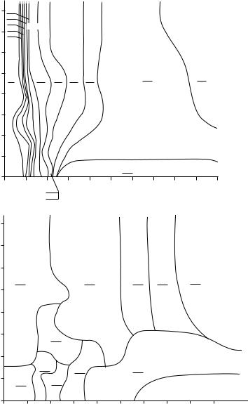
Miscellaneous Boiler Calculations |
|
331 |
||
|
TABLE 6.7 |
|
|
|
|
Summary of Results |
|
|
|
|
|
|
|
|
|
Mode of Vibration |
1 |
2 |
|
|
|
|
|
|
|
fn |
18.3 |
50.3 |
|
|
fe |
41.9 |
41.9 |
|
|
fa (Without baffle) |
54.4 |
109 |
|
|
fa (With 1 baffle) |
109 |
218 |
|
the gas velocity and fe will increase. If a baffle plate is inserted parallel to the tube length (dividing the duct width by half), then fa will double thus keeping fe and fa far apart.
Vortex shedding is unlikely to cause damage. This is due to the large mass of the system compared to the low energy in the gas stream (the analogy is a tall pole that will flex in the wind, but if it is short, it may not). Thus, using tube supports at intervals of 2–2.5 m will help reduce the vibration.
The tube natural vibration frequencies will be small in the first mode of vibration. The amplitude of vibration will be smaller at higher modes, and hence, the first mode is generally considered in the analysis.
Damping Criterion
Often, the vortex shedding frequencies coincide with the acoustic frequency, but standing waves do not develop and the transverse gas column does not vibrate. Resonance is more the exception than the rule. Chen proposed a damping criterion y based on tube geometry as follows [1]:
y = Re{(SL/d − 1)/SL/d}2 d/ST |
(6.18) |
where
ST, SL are the transverse and longitudinal spacing d is the tube outer diameter
Strouhal number S is obtained as discussed earlier. For an inline bank of plain tubes, Chen stated that y must exceed 600 before a standing wave develops. In a study on spiral finned tube bank, y reached 15,000 before sonic vibration developed. if y is less than 20,000, vibrations due to vortex shedding may not occur. Vibration analysis is not an exact science, and a lot of it is based on experience with operating units of similar design. In a few cases, the vortex shedding and acoustic frequencies were close, but no damaging noise vibration was felt.
ASME Section 3 Appendix N1330, 1995, on flow-induced vibration suggests that if reduced damping factor C exceeds 64 where
C = |
4πmz |
(6.19) |
|
ρd2 |
|||
|
|
where
m is the mass of tube, kg/m (the mass of ash deposits or fluid inside tube may be added to the tube weight)
z is the damping factor, which varies significantly (typically 0.001 for systems without intermediate supports and 0.01 with intermediate supports)
ρ is the gas density, kg/m3. d = tube OD, m


Miscellaneous Boiler Calculations |
|
333 |
|||
|
|
TABLE 6.8 |
|
|
|
|
|
Damping Factor for Evaporator Tubes |
|
|
|
|
|
|
|
|
|
|
|
Item |
Bare Tube |
Finned |
|
|
|
|
|
|
|
|
|
Gas temperature, °C |
871 |
265 |
|
|
|
Gas density, kg/m3 |
0.30 |
0.63 |
|
|
|
Gas velocity, m/s |
16.4 |
7.9 |
|
|
|
Fins/m |
Nil |
78 |
|
|
|
Fin height, mm |
— |
19 |
|
|
|
Fin thickness, mm |
— |
1.9 |
|
|
|
Tube mass, kg/m |
4.66 |
10.9 |
|
|
|
Strouhal number |
0.25 |
0.25 |
|
|
|
Vortex shed frequency, c/s |
80.8 |
38.9 |
|
|
|
Damping factor |
0.001 |
0.01 |
|
|
|
Factor C |
75.6 |
421 |
|
|
|
Natural frequency, c/s |
8.8 |
5.7 |
|
|
|
|
|
|
|
|
|
|
|
|
|
|
|
|
|
|
|
Steam Drum Calculations
Steam Velocity in Drum
When sizing steam drum internals, the chevron steam separator plays a significant role in ensuring the final steam purity (Figures 6.9 and 6.10). The boiler designer must have some idea how the steam generation varies along the length of the drum. This depends on whether we have a longitudinal gas flow boiler or a cross-flow type of boiler. If the chevron separator is located such that the steam flow enters it uniformly from all sides, then the vanes in the chevron will not be overloaded. In a steam generator, based on furnace heat loading and gas temperature profile along the convection gas path, one can obtain a good estimate of the steam generated along every meter length of the drum and then locate the chevron separator in the region where the steam generation is nearly equal from each end. This location need not be at the middle of the drum length. Similarly, in a cross-flow boiler, a large percentage of steam will be generated in the first few rows of the evaporator (due to the higher gas temperature at the inlet section), and baffling of internals has to be done considering this.
There are two vapor velocities in the drum space, which should not be exceeded to ensure that water droplets are not carried along with steam ensuring the chevron driers or vanes can perform well. Adhering to these norms will help lower the burden on the chevron separator.
The horizontal steam velocity Vh = 0.2 |
|
(ρl − ρv ) |
|
0.5 |
|
|
|
(6.20) |
|||
ρv |
|||||
|
|
|
|
|
Steam out |
|
Vv |
Chevron |
Vh |
|
|
FIGURE 6.9
Steam drum showing the flow of steam to chevron separator.

334 |
Steam Generators and Waste Heat Boilers: For Process and Plant Engineers |
3
Chevron
FIGURE 6.10
Steam drum internals. Note: (1) steam–water mixture, (2) wet steam, (3) dry stem, (4) drain pipe, and (5) belly pan.
The vertical steam velocity Vv = 0.0762 |
|
(ρl − ρv ) |
|
0.5 |
|
|
|
(6.21) |
|||
ρv |
|||||
|
|
|
|
where ρl, ρv are the densities of saturated vapor and liquid, kg/m3.
Example 6.14
A steam drum of diameter 1219 mm and length 8 m is generating 50 ton/h of steam at 40 barg. Determine the steam velocity in the vertical and horizontal directions assuming 100% of steam leaving the water line in the vertical direction and 50% enters the separator from each direction. Check if the drum cross section is reasonable.
The density of saturated water from steam tables is ρl = 1/0.00125 = 800 kg/m3 and that of saturated steam ρv = 1/0.04792 = 20.87 kg/m3.
Then, Vh should be less than 0.2 × [(800 − 20.87)/20.87]0.5 = 1.22 m/s. Vv should be less than (0.0762/0.2) × 1.22 = 0.47 m/s.
The horizontal cross section area of steam space = π × 1.2192/8 = 0.583 m2.
Volume of steam = 50,000/20.87/3,600 = 0.665 m3/s. Hence, 50% of the horizontal flow velocity = 0.5 × 0.665/.583 = 0.57 m/s, which is far below the allowable value of 1.22 m/s. Hence, it is satisfactory.
The cross section for steam flow in vertical direction = 8.5 × 1.219 = 10.36 m2 (including the dished end lengths). The average vertical velocity = 0.665/10.36 = 0.064 m/s, which is far below the allowable value of 0.47 m/s.
Hence, the drum sizing is fine. The chevron separator has to be properly selected based on allowable steam purity. One has to ensure if the holdup times specified, if any, have been met.

Miscellaneous Boiler Calculations |
335 |
Blowdown Calculations
One should perform an energy balance around the deaerator to estimate the steam for deaeration and then perform the blowdown calculations based on the conductivity (or total dissolved solids) of the boiler water, makeup water, and the feed water.
Figure 6.11 shows a simple deaerator scheme with one condensate return line. Saturated steam for deaeration is taken from the drum. Makeup water is added in the deaerator from which the feed water for the boiler is taken. By doing a mass, energy, and conductivity (or TDS) balance, we can estimate the deaeration steam.
The allowable boiler water TDS (total dissolved solids) is given by both ASME and ABMA, which are shown in Tables 6.9 and 6.10, and based on practice, one may select the appropriate value for boiler water TDS.
Example 6.15
A boiler generates 50,000 kg/h saturated steam at 20 kg/cm2 g of which 10,000 kg/h is taken for process and returns as condensate at 82°C. Makeup water is available at 21°C, and steam for deaeration is taken from the drum operating at 20 kg/cm2 g. The deaerator operates at 1.76 kg/cm2 a. Blowdown water has a TDS of 1500 ppm, and makeup has a TDS of 100 ppm. Evaluate the steam for deaeration and the blowdown.
From mass balance around the deaerator,
10,000 + D + M = F = 50,000 + B
Enthalpy of saturated steam in the drum from steam tables = 668.52 kcal/kg.
Enthalpy of makeup water at 21°C = 21.5 kcal/kg and that of condensate = 82.4 kcal/kg Saturation temperature at deaerator = 115°C. Enthalpy of feed water = 115.8 kcal/kg From energy balance around the deaerator,
10,000 × 82.4 + D × 668.52 + M × 21.5 = 115.8 × F
|
To process |
|
10,000 |
|
D |
|
50,000 |
M |
Boiler |
DA |
|
Make up |
|
|
|
|
|
|
|
|
|
|
|
|
|
|
|
|
F |
|
|
To blow down |
|
|
|
Pump |
|
|
|
||||
|
|
|
|
B |
|||||
|
|
|
|
|
|
|
|||
FIGURE 6.11
Blowdown scheme.


Miscellaneous Boiler Calculations |
339 |
Drum Holdup Calculations
Holdup time is an important parameter in steam drum design. Basically, it gives the time for all the water in the drum to evaporate at the rated steam capacity between certain levels without additional input of water from feed pump. Sometimes, distance between levels such as normal water level (NWL) and low water level (LWL) or high water level (HWL) is specified in terms of time. Then, based on these specifications, one determines the size of the steam drum.
Example 6.17
A boiler generates 50 t/h of steam at 40 kg/cm2 g (3921 kPa) (569 psig). The steam drum has an inner diameter of 1371 mm and length 10 m. Specifications call for 1.5 min of holdup time between NWL and LWL. The NWL is 50 mm below the drum centerline and the LWL is 150 mm below that. Is this adequate?
Solution
The volume of water in the drum is equal to the volume in the straight section Vs plus that in the dished ends Ve.
Vs = LR2 (a/57.3 − sina × cosa) |
(6.22) |
and
Ve = 0.261H2 (3R − H) |
(6.23) |
One must estimate the angle a as shown in Figure 6.12 for a given sector height. R = 685 mm and H1 = 635 mm and H2 = 485 mm.
a1 = cos−1(50/685) = 85.8° sin a1 = 0.9973 and cos a1 = 0.0732.
Vs1 = 10 × 0.6852 × (85.8/57.3 − 0.0732 × 0.9973) = 6.68 m3
Ve1 = 0.261 × 0.6352 (3 × 0.685 − 0.635) = 0.149 m3. With two ends, the dished end volume = 0.298 m3.
R 
a
H
L
FIGURE 6.12
Partial volume of water in boiler drum.

340 |
Steam Generators and Waste Heat Boilers: For Process and Plant Engineers |
a2 = cos−1(200/685) = 73°. sin a2 = 0.956 cos a2 = 0.292
Vs2 = 10 × 0.6852 × (73/57.3 − 0.956 × 0.292) = 4.67 m3.
Ve2 = 0.261 × 0.0.4852 × (3 × 0.685 − 0.485) = 0.096 m3. With two ends, the volume = 0.192 m3.
Total volume between the NWL and LWL = (6.68 + 0.298) – (4.67 + 0.192) = 2.11 m3. From steam tables, the specific volume of water at 40 kg/cm2 g = 0.001253 m3/kg. Hence,
the volume of water consumed at 50 tons/h steaming rate = 50,000 × 0.001253/60 = 1.044 m3/min.
Time available between the levels = 2.11/1.044 = 2.02 min. Hence, the size is adequate per specifications. In some waste heat boilers, the holdup time between NWL and empty could be as high as 5–7 min.
Estimating Flow in Blowdown Lines
The problem of estimating the discharge rates from a boiler drum or vessel to the atmosphere or to a vessel at low pressures involves two-phase flow calculations and is a lengthy procedure [5].
Presented in the following text is a simplified approach to the problem that can save considerable time for engineers who are involved in sizing or estimating discharge rates from boiler drums, vessels, or similar applications involving water. Several advantages are claimed for this approach as follows:
•No reference to steam tables is required.
•No trial and error procedure is involved for obtaining pipe size to discharge a desired rate of fluid.
•Effect of friction or equivalent length of piping can be checked.
Theory
The basic Bernoulli’s equation can be written as follows for flow in a piping system:
|
104 vdp + V2dK/2g + vdv/g + dH = 0 |
(6.24) |
|||||
Substituting mass flow rate m = V/v, |
|
|
|
|
|
|
|
|
m2/2g(dK + 2dv/v) = −104dP/v − dH/v2 |
(6.25) |
|||||
Integrating between conditions 1 and 2, |
|
|
|
|
|
|
|
m |
/2g K + 2ln(v2/v1 ) |
|
= −10 |
|
2 |
2 |
(6.26) |
|
∫dP/v − ∫dH/v2 |
||||||
2 |
|
|
|
4 |
|
|
|
|
|
|
|
|
1 |
1 |
|


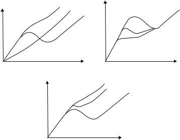

346 Steam Generators and Waste Heat Boilers: For Process and Plant Engineers
using a higher feed water temperature also helps as shown in Figure 6.15c. If inlet subcooling is eliminated, h = 0, and then Equation 6.35 becomes more stable as shown here:
P = BW2 + CW |
(6.37) |
Transient Calculations
Often, one needs to estimate the time taken to heat up a boiler knowing the flue gas flow and temperature or the tube wall temperature attained by a superheater without any flow of steam inside the tubes (say, during startup of the boiler). Lumped mass system analysis is used, which gives good estimates sufficient for practical purposes.
Gas at a temperature Tg1 enters an evaporator that is initially filled with water at a temperature of t1. The following energy balance equation can be written neglecting the heat losses:
Mcdt/dz = WgCpg (Tg1 − Tg2 ) = UA T |
(6.38) |
where
Mc is the water equivalent of the boiler = mass of steel × specific heat of steel +mass of water × specific heat of water (weight of boiler tubes, drums, and casing is included)
dt/dz is the rate of change of temperature °C/h Wg is the gas flow, kg/h
Cpg is the gas specific heat, kcal/kg°C
Tg1, Tg2 are gas temperatures entering and leaving the unit, °C. U is the overall heat transfer coefficient, kcal/m2 h °C
A is the surface area, m2
T = log mean temperature difference, °C = (Tg1 − t)− (Tg2 − t) /ln (Tg1 − t)/(Tg2 − t)
(6.39)
t is the temperature of water boiler, °C Combining with the earlier equation, we have
ln |
(Tg1 − t) |
= |
UA |
|
|
|
WgCpg |
|
|||
|
(Tg2 − t) |
|
|||
|
|
|
|
|
|
or |
|
|
|
|
|
Tg2 = t + (Tg1 − t)/eUA/WgCpg = t + (Tg1 − t)/K |
(6.40) |
||||
where |
|
|
|
|
|
|
K = eUA/WgCpg |
(6.41) |
|||
Substituting (6.40) in (6.38) and simplifying, we have |
|
||||
Mcdt/dz = WgCpg (Tg1 − t)(K − 1)/K |
(6.42) |
||||
Miscellaneous Boiler Calculations |
|
|
347 |
or |
= WgCpg (K − 1)/McK dz |
|
|
dt/(Tg1 − t) |
(6.43) |
||
|
|
|
|
Integrating from time t1 to t2, we have |
|
|
|
ln[[(Tg1 − t1)/(Tg1 − t2 )] = [WgCpg (K − 1)/(McK)]z |
(6.44) |
||
This equation gives an idea of the time required to heat up the boiler from temperature t1 to, say, the boiling temperature of 100°C. Once steam starts forming additional equations for latent heat, flow-through vent may be developed to obtain a more accurate startup curve.
Example 6.19
A waste heat boiler weighs 50,000 kg and contains 30,000 kg of water at 27°C. To the boiler enters 130,000 kg/h of flue gases at 800°C. Assuming that gas specific heat = 0.3 kcal/kg°C, steel specific heat = 0.12 kcal/kg°C, surface area for heat transfer = 2000 m2, and overall adjusted U = 40 kcal/m2 h °C, determine the time taken to heat the boiler with the water to 100°C.
Solution: |
|
|
|
UA/WgCpg |
= 40 × 2,000/(130,000 × 0.3) = 2.05. K = e2.05 = 7.78 |
||
Mc = 50,000 × 0.12 + 30,000 × 1 = 36,000 |
|
||
|
|
|
|
ln (800 − 27)/(800 − 100) |
= 0.099 = 130,000 × 0.3 × (7.78 |
− 1)/36,000/7.78 z |
|
|
|
= 0.944z or z = 0.1 h or 6 min |
|
One has to then check the time for generating steam and ensure if the superheater gas inlet temperature is reasonable. In practice, some differences may be seen due to the assumptions made such as a uniform U for the complete evaporator; the drums may have a lower value of U compared to the tubes.
Example 6.20
The time required to heat up a superheater in a gas turbine exhaust plant from 27°C to 480°C has to be determined. At 550°C, 68,000 kg/h of turbine exhaust gases enter the HRSG. Assume the gas-side heat transfer coefficient is 60 kcal/m2 h °C, gas specific heat = 0.286 kcal/kg°C, weight of the superheater is 2000 kg, and surface area = 180 m2.
Solution
|
Mc = 2000 × 0.12 = 240 kcal/°C |
|
Using Equations 6.41 and 6.44, |
|
|
K = exp 60 × 180 / |
(68,000 × 0.286) = exp(0.555) = 1.74 |
|
|
|
− 1)z/1.74/240 or z = 0.058 or 3.6 min. |
ln (550 − 27)/(550 − 480) = 68,000 × 0.286 × (1.74 |
||
|
|
|
This gives an idea of how fast the metal gets heated up. The steam generation based on the calculations done as in earlier example may take much longer than 3.6 min. If the startup is frequent, one can start up the gas turbine on low load when the exhaust gas temperature will be much lower. This is the reason that with high gas inlet temperatures,
348 |
Steam Generators and Waste Heat Boilers: For Process and Plant Engineers |
the superheater is shielded from the hot gases by a screen section that reduces the gas temperature entering it. Else, it can get oxidized without flow of steam. In fired boilers, the firing rate is controlled to keep the gas temperature lower at the superheater inlet if it is a radiant superheater. Here again, a convective superheater with a screen section helps.
Example 6.21
With 450°C exhaust gas temperature and the same gas flow (no bypass stack), what temperature will the tube metal reach in 10 min?
ln[(450 − 27)/(450 − t)] = 68,000 × 0.286 × 0.74 × 0.167/(1.74 × 240) = 5.75 or t = 449°C. The superheater will reach the gas temperature in about 10 min. In 5 min, the tubes will attain 425°C. It is likely that steam will start flowing through the tubes within 10 min. As discussed in Appendix E, the finned evaporator weighs less and is compact, and hence, the water equivalent is lower compared to plain tube boilers, and hence, this helps to speed up the steam generation.
Analysis of an Evaporator
In an evaporator, the large mass of metal and water inventory results in a longer startup time, but the residual energy in the metal also helps to respond to load changes faster when the energy from flue gas or heat input to the boiler is cut off. Drum-level fluctuations are also smoothed out by a large water inventory.
The basic equation for energy transfer to the evaporator is
Q = Wshfg + (hl − hf )Wf + (WmCpdt/dp + Wwdh/dp)dp/dz |
(6.45) |
where
Wm is the mass of metal, kg
Ws, Wf are mass flow of steam, feed water, kg/h
Ww is the amount of water inventory in the boiler system including drums, tubes dh/dp is the change of enthalpy to change of steam pressure, kcal/kg/kg/cm2
dt/dp is the change of saturation temperature change to change in pressure, °C/kg/cm2 Q is the energy transferred to evaporator, kcal/h
dp/dz is the rate of pressure change, kg/cm2/h
Let the steam space between the drum level and the first valve = V m3. The change in pressure may be written as
pv = C = pV/m where C is a constant
m is the mass of steam, kg in volume V or, pV/m = C
or |
|
dp/dz = (pv/V)(Ws − Wl ) |
(6.46) |
where
p is the steam pressure
Ws, Wl are the steam generated and the steam withdrawn by process
When steam withdrawn is equal to steam generated, the steam pressure is unchanged. Pressure fluctuations occur when the steam generated and steam demand differ.
350 |
Steam Generators and Waste Heat Boilers: For Process and Plant Engineers |
From (6.45), 20,400×(261.7 − 105.8) + Ws × 405.3 + 21,030dp/dz = 11.67 × 10⁶ also, dp/dz = 0.62 × (Ws − 22,686)
3.18 × 10⁶ + 405.3Ws + 21,030 × 0.62 × (Ws − 22,686) = 11.67 × 10⁶ 13,443.9Ws = 295.79 × 10⁶ + 8.49 × 10⁶ or Ws = 22,630 kg/h
Thus, dp/dz = 0.62 × (22,630 − 22,686) = −35 kg/cm2/h = −0.01 kg/cm2/s (pressure falls slightly)
Case 2:
13,443.9Ws = (295.79 + 11.67)× 106 or Ws = 22,869 kg/h
dp/dz = 0.62 × (22,869 − 22,686) = 113 kg/cm2/h = 0.0315 kg/cm2/s
The pressure actually increases because the cooling effect of the feed water is not sensed. In practice, controls respond fast and restore the balance among heat input, feed water flow, and steam flow. The preceding equations represent the worst-case scenario when controls do not act. If we do not adjust the heat input, the steam pressure will slide if we withdraw more steam than generated. The preceding equations may be used to show the trend and are simplistic models. Programs can be developed for more accurate modeling of transients in any steam generator.
Drum-Level Fluctuations
In cogeneration plants, the process conditions dictate the steam demand and could vary a lot from normal operating conditions. When the steam demand suddenly increases in a boiler, it may take a few milliseconds to a few seconds depending on the control system to adjust the flow and energy input to match the demand. When the evaporation rate in a boiler increases suddenly, water from the boiler tubes is displaced into the drum, which raises the water level momentarily or causes the swell effect. Momentarily, the pressure is also reduced. This swell occurs whether the increased evaporation is due to heat transfer in boiler surfaces or due to self-boiling as a result of falling steam pressure due to higher than ongoing steam generation. Similarly, a shrink effect occurs when the steam demand decreases and water level decreases momentarily. The change in water level is proportional to the change in evaporation. The effect of feed water flow will also have to be considered. The mass of water in the drum increases at the following rate:
[(Wi − Ws) + T (Ws − Wl)/dt]
where T is the mass of water displaced into drum by unit increase in evaporation = 3600 × water weight × (hl − hfw)/[Ws × (hv − hfw)], where Wi, Ws, Wl are the water flow in, normal steam generation, and steam withdrawn in kg/h, respectively.
If water inventory = 40,000 kg in a boiler and from steam tables hl = 198, hfw = 105, hv = 665 kcal/kg, and Ws = 18,000 kg/h, then T = 3,600 × 40,000 × (198 − 105)/[18,000 × (665 − 105)] = 1,328 s. In a steady-state situation, Ws = Wl = Wi (neglecting blowdown). Then,
dh/dt = level change/s = v[(Wi − Ws + T(Ws − Wl)/t]/A
where
A is the drum cross section, m2
v is the specific volume of saturated liquid, m3/kg

Miscellaneous Boiler Calculations |
351 |
Example 6.24
If in the boiler mentioned earlier, steam demand suddenly changes from 18,000 to 21,000 kg/h in 7 s, and if A = 10 m2, v = 0.001125 m3/kg, then momentary change in level = 0.001125 × [1,328 × 3,000/3,600/7]/10 = 0.0177 m/s = 17.7 mm/s, which is significant assuming controls do not react immediately. In practice, the swell will be much smaller and will last for a much shorter period, say, for a few milliseconds with good controls such as three-element-level control system.
Fan Calculations
Density of air or flue gas has to be obtained first to perform fan-related calculations.
Density of Flue Gas, Air |
|
The following formula may be used to estimate the density of air and flue gases: |
|
ρ = MW× P/8314/T |
(6.47) |
where
MW is the molecular weight of flue gas P is the pressure of flue gas, air in Pascal T is the temperature, K
ρ is the gas density, kg/m3
For dry air, MW = 28.97. (8314 is the universal gas constant)
At 273 K, at sea level, and at atmospheric pressure (101,325 Pa), density of dry air is
ρ = 28.97 × 101,325/273/8,314 = 1.293 kg/m3
In British units, from Table 6.11, ρ = 0.0933 × 28.97 × 14.7/(460 + 32) = 0.08076 lb/ft3 = 1.292 kg/m3. Effect of elevation on the density of air is given in Table 6.12, and Table 6.13 shows the molecular weight of some gases.
A simplified formula for the estimation of air density at atmospheric pressure, at sea level, and at a temperature of T K is
ρ = 353/T |
(6.48) |
At 300 K, density of air = 353/300 = 1.177 kg/m3 = 0.0735 lb/ft3
Example 6.25
Flue gas at 100°C (212°F) having the following analysis % volume CO2 = 15, H2O = 8, N2 = 75, O2 = 2 at a 200 mm wc (1961 Pa) (7.9 in. wc) gauge pressure and at 1000 m (3280 ft) elevation flows inside a boiler plant duct. Determine the density.
Correction factor from Table 6.12 is 0.887 by interpolation. MW of flue gas = 0.75 × 28 +
.02 × 32 + 0.15 × 44 + 0.08 × 18 = 29.68
Gas pressure = 101,325 × 0.887 + 1,961 = 118,446 Pa
ρ = 29.68 × 118,446/8314/373 = 1.133 kg/m3 (0.0708 lb/ft3 )
Hence, if 100,000 kg/h of flue gas flows in a duct at these conditions, the volume of flue gas = 100,000/1.133 = 88,261 m3/h.

352 |
Steam Generators and Waste Heat Boilers: For Process and Plant Engineers |
|||
|
TABLE 6.11 |
|
|
|
|
Density of Flue Gas, Air |
|
|
|
|
|
|
|
|
|
SI |
British |
Metric |
|
|
|
|
|
|
|
ρ = 1.203 × 10⁻⁴ MW P/T |
ρ = 0.0933 MW P/T |
ρ = 11.792 MW P/T |
|
|
P is the absolute pressure, Pascal |
psia |
kg/cm2 a |
|
|
T, K |
T, °R |
T, K |
|
|
ρ, kg/m3 |
ρ, lb/ft3 |
ρ, kg/m3 |
|
Note: MW is the molecular weight of gas.
TABLE 6.12
Density Correction Factor
Elevation, m (ft) |
Correction |
|
|
0 |
1 |
305 (1000) |
0.964 |
610 (2000) |
0.930 |
915 (3000) |
0.896 |
1220 (4000) |
0.864 |
1524 (5000) |
0.832 |
1829 (6000) |
0.801 |
2134 (7000) |
0.772 |
2439 (8000) |
0.743 |
|
|
TABLE 6.13
Molecular Weight of Gases
Gas |
MW |
Gas |
MW |
|
|
|
|
Hydrogen |
2.016 |
Ammonia |
17.03 |
Oxygen |
32.0 |
Carbon dioxide |
44.01 |
Nitrogen |
28.016 |
Carbon monoxide |
28.01 |
Air (dry) |
28.97 |
Nitrous oxide |
44.02 |
Methane |
16.04 |
Nitric oxide |
30.01 |
Ethane |
30.07 |
Nitrogen dioxide |
46.01 |
Propane |
44.09 |
Sulfur dioxide |
74.06 |
n-Butane |
58.12 |
Sulfur trioxide |
80.06 |
Water vapor |
18.02 |
|
|
|
|
|
|
Pressure Drop in Ducts
In steam generators or waste heat boilers, one often has to estimate the air or flue gas pressure drop in ducts given the flue gas analysis and temperature. The Reynolds number has to be determined first from the following formula:
Re = 1.273w/(diµ) where w is the flow in kg/h, µ is the viscosity in kg/m h, and di is the equivalent diameter of duct, m (see Table B.1).
Miscellaneous Boiler Calculations |
353 |
Example 6.26
Determine the flue gas pressure drop in a rectangular duct with a cross section of 0.6 × 0.75 m. Flue gas flow is 11,300 kg/h at 150°C. Assume natural gas products of combustion and total developed length of 30 m. Flue gas from combustion of natural gas has the following analysis in % volume: CO2 = 8.29, H2O = 18.17. N2 = 71.08, O2 = 2.46. MW = 27.6
Solution
The duct equivalent diameter = 2ab/(a + b) = 2 × 0.6 × 0.75/1.35 = 0.666 m
Re = 1.273 w/diµ. The flue gas viscosity at 200°C from Table F.7 is 0.0789 kg/m h. Hence, Re = 1.273 × 11,300/(0.666 × 0.0789) = 276,240
Use the Blasius friction factor correlation. Friction factor f = 0.316/Re0.25 = 0.0138 Density of flue gas at atmospheric pressure = 12.17 × 27.6/(273 + 150) = 0.794 kg/m3 From Table B.6, P = 6.382 × 10⁻⁹ f Le v w2/di5 = 6.382 × 10⁻⁹ f Le v w2/di5 = 6.382 × 10−9 × 0.0138 × 30 × 11,3002/(0.794 × 0.6665) = 3.3 mm wc
Fan Selection
Package steam generators generating up to 120 tons/h of steam today use a single fan. The furnaces of oiland gas-fired boilers are pressurized. Estimating the flow or head inaccurately can lead to operation of the fan in an unstable region or result in the horsepower being too high and the operation inefficient. The inlet density of air and the flow volume and temperature should be estimated accurately considering flue gas recirculation (FGR) if any. If flue gas at, say, 150°C is with ambient air and sent to the fan inlet, the density will be lower as the mixture temperature is higher than ambient temperature. The flow volume will also be higher considering the amount of flue gas recirculated. In addition, the elevation factor should be kept in mind. The fan is selected for the lowest density case as the fan always delivers the same volume, and hence, the mass flow is lower at lower density. Ensuring the required mass flow of air for combustion at the lowest density case will result in higher mass flow of air at higher density cases (say, lower ambient temperatures). The fan also delivers a lower head at lower density, while the steam generator may require a constant head due to a given mass flow of flue gas at a particular load. Hence, provision should be made to turn down the fan under such circumstances. The effect of air density on fan performance is shown in Figure 6.16.
One of the mistakes made by consultants or plant engineers is the use of large margins on flow and head. This leads to oversizing of the fan (considering that a single fan is often used) and operation close to the unstable region as shown in Figure 6.16 at part loads. Fan also will have a large motor, which is unnecessary. Typically, 10% margin on flow and a maximum of 15%–20% on head should be adequate for package boilers. Else, inlet vane control and variable speed drives may be required for the turndown making the fan system expensive. In a large utility boiler, two or even three fans are used, and when the turndown is low, say, 50%, a fan may be cut off. With a single fan system, this results in operation at low flows, and hence, the excess air control becomes difficult. Underestimating the fan head can also cause the fan to operate in the unstable region as shown in Figure 6.16a. The fan operating point should always be in the negatively sloping portion of the head versus flow curve; else, the fan could operate in the unstable region causing surges and vibration.
The fan inlet duct and downstream ductwork to the burners must have proper flow distribution. Pulsations and duct vibrations are likely if the inlet air flow to the fan blades is not smooth.

Miscellaneous Boiler Calculations |
355 |
Head Developed by Fan
A fan always develops the same volume and same head Ha in height of air column, but the pressure will vary depending on density. We can also write Ha ρa = Hw ρw, where Hw is the head developed in mm wc and ρw is the air density. It is a practice in the industry to work with Hw for fan as it is easy to measure. Hence, Ha = Hw ρw/ρa.
As density of water ρw is the same, we can use the following expression to understand how the fan head varies with air density:
Hw1/ρ1 = Hw2/ρ2
Hence, a fan will develop a lower head of water column at lower density. The flue gas pressure drop across boiler heating surfaces is calculated in mm wc (see Chapters 2, 3, and 5). Hence, we have to ensure that the fan can handle to flue gas pressure drop at the lowest air density case. Figure 6.16c also illustrates that.
Fan Power Consumption
P = Hw Q/ηf ηm where Hw is the total pressure developed in Pa, P the power consumption in watts, ηf, ηm the efficiency of fan and motor in fractions, and Q is the volumetric flow in m3/s. Converting to mass units,
P = HwW/( ρηfηm )
If Hw is the head developed in mm wc (which is often used in boiler practice and in measurements), multiply it by 9.807 to obtain head in Pascal.
Example 6.27
A steam generator requires 8.5 m3/s (18,000 cfm) air at 30°C for combustion. Static head required is 457 mm wc (18 in. wc). Fan and motor efficiencies are 75% and 90%, respectively. Determine the motor power consumption.
P = 9.807 × 457 × 8.5/0.75/0.9 = 56,437 W = 56.5 kW
Density assuming atmospheric pressure is 1.165 kg/m3. Hence, mass flow is about 8.5 × 1.165 = 9.9 kg/s (78,560 lb/h)
Estimating Stack Effect
Whenever flue gas flows inside a tall vertical stack, a natural draft is created owing to the difference in density between the low density flue gas and ambient air, which has a higher density. Due to the friction loss inside the stack, the available draft is reduced. The estimation of available draft assumes significance in small boilers operating without forced or induced draft fans.
Example 6.28
Determine the stack effect when 50,000 kg/h of flue gas at 200°C from the combustion of fuel oil flows inside a 1.22 m diameter stack of height 16 m. Flue gas analysis is % volume CO2 = 11, H2O = 12, N2 = 74.5, O2 = 2.5. Ambient air is at 25°C.

356 |
Steam Generators and Waste Heat Boilers: For Process and Plant Engineers |
Neglect the effect of elevation and gas temperature in the stack. Gas pressure is atmospheric. MW of flue gas = 28.66 × 101,325/8,314/473 = 0.738 kg/m3. Density of air = 353/298 = 1.185 kg/m3
Available draft = (1.185 − 0.738)× 16 = 7.15 kg/m2 = 7.15 mm wc
Friction loss in stack:
P = 0.08262 f Le v w2/di5 from Appendix B, where P is in mm wc.
w= flow in kg/s = 50,000/3,600 = 13.9 kg/s
v = specific volume of fluegas at 200C = 1/0.738 = 1.355 m3 /kg
To estimate the friction factor, first the Reynolds number is computed. From Appendix F, viscosity of flue gas at 200°C is 0.0863 kg/m h = 2.397 × 10⁻⁵ kg/m s. Reynolds number is obtained from Appendix B as follows:
Re = 1.273w/d/µ = 1.273 × 13.9/1.22/2.397 × 10−5 = 6.05× 10⁵
Friction factor in turbulent regime may be estimated using f = 0.316/Re0.25 = 0.011
P= 0.08262 × 0.011× 16 × 13.92/1.225 = 1.039 mm wc Net draft available = 7.15 − 1.039 = 6.1 mm wc
References
1.D.Q. Kern, Process Heat Transfer, McGraw-Hill, New York, 1950, p263.
2.K.O. Beatty and D.L. Katz, Condensation of vapors outside of finned tubes, Chemical Engineering Progress, 44.1, 55–70, 1948.
3.Century Brass Products, Heat Exchanger Manual, Waterbury, CT, 1950.
4.V. Ganapathy, Avoid heat transfer equipment vibration, Hydrocarbon Processing, June 1987, p62.
5.F.J. Moody, Maximum two-phase vessel blowdown from pipes, Transactions of ASME, Journal of Heat transfer, August 1966, 285.

358 |
Appendix A: Boiler Design and Performance Calculations |
calculations, thermal and transport properties of flue gases play a vital role, and methods of estimating these are shown in Appendix F. Some practice with these calculations will help engineers evaluate the performance of their steam generators or waste heat boilers or any of the boiler components such as superheater, evaporator, or economizer or fire tube waste heat boiler or air heater with ease and see if the operating data are close to that predicted by the boiler supplier or not or whether a potential problem exists. Detailed calculations with real-life examples are given throughout the book so one may develop computer code for faster and more accurate calculations. Depending solely on the boiler supplier to perform these studies may not often be a good idea. Often, the reports from the boiler suppliers can be biased; the plant engineer can then challenge them if he can independently perform these studies. This is the main objective of this book; to educate plant and process engineers on boiler related applied heat transfer calculations so that they can arrive at the performance of various boiler components or that of the entire steam generator or HRSG independently. When there is a problem in a steam generator or HRSG, it is easy to shift the blame on poor operation or maintenance, while the real issue could be the poor design of the steam generator. Hence, plants with steam generators and waste heat boilers should develop in-house talent to perform thermal performance calculations, and this book provides tools for that very purpose. The information provided will also be pertinent to boiler suppliers.
Basic Equations for Energy Transfer
The total energy transferred Q in kW in a convective heat transfer equipment such as a superheater, evaporator, or economizer is given by the following basic equation:
Q = U A T |
(A.1) |
T is the corrected log-mean temperature difference (LMTD), K. If surface area A is based on external surface area, then U is also based on external surface area. If A is based on tube inner diameter, then U is based on tube ID. The relation between the two is simple:
UoAo = UiAi |
(A.2) |
where
Uo and Ui are the overall heat transfer coefficients based on external and internal surface areas
Ao and Ai are the external and internal surface areas of the tubes
If external radiation Qr from a cavity, flame, or furnace is received by the heat transfer surface, then the preceding equation is modified as
Q − Qr = Qc + Qn = U A T |
(A.3) |
where Qc, Qn are the energy transferred by convection and nonluminous radiation, kW.
Appendix A: Boiler Design and Performance Calculations |
359 |
In addition to the above equation, energy balance equations should also be satisfied. The energy given by the hot fluid, namely, the flue gases, has to be absorbed by the colder fluid, say, water (in an economizer) or steam (in a superheater) or by air (air heater) or steam water mixture (boiler evaporator).
Wh hh (1− hl ) = Wc hc = Q |
(A.4) |
where
Q is the energy transferred in kW. Qr is neglected when direct radiation from furnace or cavity is absent or when gas temperature is low, say, less than about 700°C. Chapter 2 discusses the method of estimating Qr
A = surface area, m2
W is the fluid flow or flue gas flow, kg/s (subscripts c and h stand for cold and hot fluids) h is the change in enthalpy, kJ/kg (subscripts h and c stand for hot and cold side fluids) = Cp × temperature change, where Cp is the specific heat, kJ/kg K
Correction factors for LMTD for different types of arrangement such as parallel-flow, cross-flow, and counter-flow are available in reference books. In pure counter-flow or par- allel-flow, it is 1. For cross-flow arrangements, charts are available. See Figure A.1 [1].
hl is the heat loss, ranging from 0.2% to 1%. The method of evaluating this is explained in Chapter 6 on miscellaneous calculations; heat loss depends on the type of boiler casing, insulation thickness, ambient temperature, and wind velocity conditions.
Table A.1 shows the different systems of units that have been used in this book. One can easily perform the calculations in any system of units.
For extended surfaces, Uo may be obtained as follows [2]:
1 |
|
At |
|
At |
|
At |
|
d |
|
d |
|
1 |
|
||
|
= |
|
+ ffi |
|
+ |
|
|
|
|
ln |
|
|
+ ffo + |
|
(A.5) |
Uo |
(hiAi ) |
Aw |
|
|
ηho |
||||||||||
|
|
Ai |
|
|
2Km |
di |
|
|
|||||||
where
At is the total external surface area of finned tube per unit length, m2/m Ai is the tube inner surface area per unit length = πdi, m2/m
Aw is the average wall surface area = π(d + di)/2, m2/m
Km is the thermal conductivity of tube wall (see Appendix E for properties of some boiler tube materials)
d, di are the tube outer and inner diameters, m
ffi, ffo are the fouling factors inside and outside tubes, m2 K/W
hi, ho are the tube inside and outside side heat transfer coefficients, W/m2 K η is the fin effectiveness, fraction
If plain or bare tubes are used, the preceding equation may be simplified and written as follows:
1 |
|
d |
|
d |
|
d |
|
d |
|
1 |
|
|||
|
= |
|
+ ffi |
|
|
+ |
|
|
ln |
|
|
+ ffo + |
|
(A.6) |
|
|
|
|
|
||||||||||
Uo |
hidi |
|
|
ho |
||||||||||
|
di |
|
2Km |
di |
|
|
||||||||


362 |
Appendix A: Boiler Design and Performance Calculations |
Using hi = 1500 W/m2 K (264 Btu/ft2 h °F), we can show that Uo = 72 W/m2 K (12.67 Btu/ft2 h °F), still close to ho. If extended surfaces are used, then U will again be close to the corrected outside coefficient ηho.
Let us say we have an economizer that uses solid fins of density 78 fins/m (2 fins/in.), 19 mm high (0.75 in.), and 1.5 mm (0.059 in.) thick alloy steel fins. The ratio of external to internal surface can be shown to be 5.2. Assume hi = 8000 W/m2 K (1408 Btu/ft2 h °F). The other data are as in previous example. Due to the use of fins, the gas-side heat transfer coefficient will decrease. Use, say, 60 W/m2 K for corrected gas-side heat transfer coefficient (ηho) and a fin effectiveness of 84% (ho will be lower for finned tubes compared to plain tubes for the same gas velocity. This is discussed later in Appendix E). Then,
1/Uo = 5.2/8000 + 1/60 + 5.2 × 0.05/2/43 × ln(0.05/0.042) + 0.000175 + 0.000175 × 5.2 = 0.0394 or Uo = 52.8 W/m2 K (9.29 Btu/ft2 h °F)
which is again close to the corrected outside coefficient of 60 W/m2 K (10.56 Btu/ft2 h °F).
Fire Tube Boilers, Gas Coolers, Heat Exchangers
In these equipment, the flue gas flows inside the tubes while a fluid with high heat transfer coefficient is on the shell side.
Here let us use the same values for ho and hi and tube sizes, namely, hi = 50 W/m2 K (8.8 Btu/ft2 h °F), ho = 8000 W/m2 K (1408 Btu/ft2 h °F). Tube OD × ID = 50 × 42 mm. From (A.6),
1/Uo = 0.05/0.042/50 + 1/8000 + (0.05/43/2) ln(0.05/0.042) + 0.000175 + 0.000175 × 0.05/0.042 = 0.0243 or Uo = 41 W/m2 K (7.22 Btu/ft2 h °F) (based on outer surface area).
Converting to tube inner diameter basis, we have the following relation:
Uo × d = Ui × di or Ui = 41× 50 = 48.8 W/m2 K or very close to hi. 42
Hence, in fire tube boiler also, the gas-side coefficient governs U. The gas-side coefficient governs the overall heat transfer coefficient in evaporators, superheaters, and economizers and fire tube boilers. One should also note that when we specify the U value, we should state whether it is based on inner or outer diameter of the tube.
Gas to Gas Exchangers: Air Heater
In the case of air heaters, both the tube side and outside coefficients have to be considered in determining U as both coefficients are comparable in value unlike in boilers or economizers where the gas-side coefficient was so small compared to the steamor water-side coefficient.
If hi = 50 W/m2 K (8.8 Btu/ft2 h °F)and ho = 60 W/m2 K (10.56 Btu/ft2 h °F),then from(A.6)
1/Uo = 50/42/50 + 1/60 + (0.05/2/43) ln(50/42) + 0.000175 + 0.000175 × 50/42 = 0.04096 or Uo = 24.4 W/m2 K (4.22 Btu/ft2 h °F). This is close to neither hi nor ho. The same conclusion

Appendix A: Boiler Design and Performance Calculations |
363 |
may be drawn in the case of liquid to liquid exchangers where both the tube inside and outside coefficients are large and comparable, and so both will influence Uo.
Thus, in boiler performance analysis, one has to keep in mind that the evaluation of the gas-side heat transfer coefficient assumes significance when it comes to evaluating the performance of superheaters, economizer, or boiler bank tubes or evaporator and greatly impacts their performance or duty. However, it is also essential to compute the tube-side coefficients to estimate the tube wall temperature accurately as in the case of superheaters. This helps in the selection of proper materials or warns us if low-temperature corrosion is likely in case of an economizer or air heater.
Design and Performance Calculations
Two types of calculations are done for any heat transfer equipment.
Design Calculation
In this process, the tube geometry (such as tube size, spacing of tubes, fin geometry, if any) is first assumed, then U is computed based on gas and steam–water parameters, and finally the surface area of the superheater or evaporator or economizer is arrived at based on the duty or energy required to be transferred and the LMTD. In design case, the mass flows of flue gas and steam or water and the temperatures at inlet and exit of both streams and the duty Q are known. U, the overall heat transfer coefficient, LMTD ( T), the log-mean temperature difference are computed, and then the required surface area A is obtained; then one checks if the geometry (tubes/row, length, fin configuration, rows deep) and other aspects such as tube wall temperatures, gas pressure drop, and space requirements are reasonable. If not, the configuration is changed, and the calculations are redone. The flue gas tube-side fluid parameters chosen for the design condition are important; it could be the maximum duty case or the load at which the equipment is likely to operate most of its lifetime. There is only one design condition. Note that in the design case, the LMTD ( T) is known, as we know from heat balance the flue gas and steam/water inlet and exit temperatures; U is computed based on gas and fluid data and tube geometry data, and A is the only unknown. This procedure is applicable to any heat transfer component whether flue gas flows inside or outside the tubes. The steps are as follows:
•Assume exit temperature of either stream, say, T2, the hot gas stream.
•Compute the assumed duty Qa = W × Cp × (T1 − T2).
•Compute the exit temperature of the cold fluid using preceding duty. Since the mass flow is known, one can check the enthalpy difference and then the temperature change.
•Compute LMTD as now all four temperatures are known.
•Tube sizes, tube spacing, length, cross section of the equipment, and fin geometry, if any, have to be assumed. Using the procedure described in Appendices B through E, the various heat transfer coefficients are computed and then U.
•Estimate the surface area required using A = Qa/(U T) = NwNdLAt, where Nw, Nd, L, and At are the number of tubes wide, deep, tube length, and surface area per unit length.

364 |
Appendix A: Boiler Design and Performance Calculations |
•Check the number of rows deep required from the above step.
•Check the gasand steam-side pressure drops, and if they are not reasonable, then repeat the exercise using different cross sections or tube geometries and finalize the tube geometry.
Off-Design or Performance Calculation
The off-design calculations are done to check how the given equipment performs at other gas or steam parameters, part loads, or how the boiler will perform with different fuels, steam pressures, excess air, at different flue gas recirculation rates, and so on. The tube geometry and surface area details are known. There can be numerous offdesign conditions for a boiler component. In an HRSG, the design case may be the unfired 100% gas turbine load case and the off-design case could be the supplementary fired 70% gas turbine load case with import steam. Steam pressure or feed water temperature may also change. There are numerous possibilities, and the plant has to inform the boiler supplier of the possible operating modes. For example, if a boiler is fired with natural gas and then switched to a low BTU fuel, then the flue gas flow through the boiler can increase by about 60%–70%, which results in a different gas and steam temperature profile along the gas path and high back pressure through the boiler. Fans have to be checked to see if they can handle the high flue gas quantity. Off-design calculations are done in advance to check these issues. Plant engineers have a large role to play here as they know about the needs of the plant. If they miss something and the boiler designer does not consider that piece of information, then the design may be in jeopardy.
Though design calculations are performed by the boiler supplier, the procedure is discussed in case the plant engineer has to come up with the redesign of a boiler component due to changes in some parameters. Or the procedure may also be used to check the sizing done by the boiler vendor.
Superheater Design and Off-Design Calculation
We will now illustrate the design and off-design calculations for a finned tube superheater (Figure A.2). One may refer to Appendix E, where the U value is evaluated for this superheater.
Example A.1
A 50.8 × 44 mm (2 × 1.732 in.) solid finned superheater with 78 fins/m (2 fins/in.), 12.7 mm (0.5 in.) high fins, and 1.52 mm (0.06 in.) thick is arranged in inline fashion with 101.8 mm (4 in.) square pitch: 18 tubes/row, 6 rows deep, 3.1 m (10.2 ft) long tubes with 9 streams. Gas flow is 100,000 kg/h (220,400 lb/h) with the following exhaust gas analysis by volume% CO2 = 3, H2O = 7, N2 = 75, O2 = 15. The bundle is designed with inlet and exit exhaust gas temperatures of 550°C (1022°F) and 479°C (892°F) and with 25,000 kg/h (55,100 lb/h) of saturated steam at 51 kg/cm2 g (725 psig) raised from saturation temperature of 265°C (509°F) to 369°C (696°F). Surface area is 188 m2 (2030 ft2). Check if the design is reasonable. Flue gas data from Appendix F at the average gas temperature of 514°C have been estimated as follows: Cp = 0.2755 kcal/kg °C (0.2755 Btu/lb °F), µg = 0.127 kg/m h (0.085 Btu/ ft h), kg = 0.0468 kcal/m h °C (0.0314 Btu/ft h °F). Assume 1% heat loss.

Appendix A: Boiler Design and Performance Calculations |
365 |
Gas in
Steam
out
Steam
in
Gas out
FIGURE A.2
Typical convective superheater.
Solution
First let us check the design.
The exit gas temperature is 479°C. The duty is then
Q = Wg × Cpg × (Tg1 − Tg2) × (1 − hl) = 100,000 × 0.2755 × (550 − 479) × .99 = 1.936 × 10⁶ kcal/h (7.68 MM Btu/h) (2.25 MW).
Enthalpy absorbed by steam = 1.936 × 10⁶/25,000 = 77.4 kcal/kg (139.3 Btu/lb). From steam tables at 51.5 kg/cm2 of steam pressure, saturated steam enthalpy from steam tables is 667.3 kcal/kg (steam-side pressure drop of 1.5 kg/cm2 was assumed); exit enthalpy = 667 + 77.4 = 744.7 kcal/kg. Hence, exit steam temperature = 368°C (694°F).
For counter-flow arrangement,
T = [(479 − 265) − (550 − 368)]/ln [(479 − 265)/(550 − 368)] = 197.6°C (355°F).
Uo from Appendix E is 51.9 kcal/m2 h °C (10.6 Btu/ft2 h °F).
Surface area required A = 1.936 × 10⁶/197.6/51.9 = 189 m2 (2033 ft2). Surface area provided is 188 m2 (2023 ft2). Hence, the duty is close to that assumed, and the design is reasonable. If U is not given, then one may use the methods discussed in Appendices B through E to arrive at U.
What if the plant engineer is asked to design a superheater from scratch for a specific duty or parameters? In such cases, the following points may be kept in mind.
1.Calculate the duty of the superheater as we know the mass flow of steam and its inlet and desired exit temperatures; evaluate the flue gas exit temperature. The flue gas mass flow should be known or will be available. Then, the LMTD is computed as all the four temperatures are known.
2.The cross section of the superheater should be selected such that the gas velocity is in the range of 20–35 m/s (for dust-laden gases, the velocity will be much lower, say, around 10–20 m/s). Values beyond the range may sometimes be

366 |
Appendix A: Boiler Design and Performance Calculations |
acceptable due to layout and shipping considerations. The gas pressure drop will have to be checked later and should be within allowable values; if not, the cross section is revised.
3.Streams should be selected on the tube side such that the steam-side velocity is in the range of 15–30 m/s depending on steam pressure and pressure drop. At lower pressure, the specific volume of steam is higher and so the velocity. For a discussion on streams, refer to Appendix B.
3.Calculate hc, hn, hi, and U using the methods described in the appendices.
4.Using the equation Q = UA T, determine A and the number of rows deep as before.
5.Compute the gasand steam-side pressure drops as shown in Appendices B and C and see if they are reasonable. If not, repeat from step 2 by manipulating the tube length, size, or length or tube spacing.
Performance Evaluation
There are two ways of doing off-design performance evaluation for any heat transfer component without phase change such as superheater or economizer. The following information should be available in a plant for any equipment: gas flow, inlet gas temperature, surface area of exchanger, and steam or water flow and its inlet temperature. The performance has to be evaluated. By performance, we mean the duty, exit temperatures of both fluids, pressure drops on gas and steam side, and tube wall temperatures.
Conventional Method
•Assume exit temperature of either stream, say, the hot gas stream, T2.
•Compute the assumed duty, Qa = W × Cp × (T1 − T2).
•Compute the exit temperature of the cold fluid using preceding duty from energy balance. Since the mass flow is known, one can compute the enthalpy difference and then the exit temperature of the cold fluid.
• |
Compute LMTD, T as now all four temperatures are known. |
• |
Compute U using average fluid or film temperatures as appropriate. |
• |
Compute the transferred duty using Qt = UA T. |
•If both Qa and Qt are within a desired margin, say, 0.5%, then iterations stop, and all the values of duty and temperatures are frozen; if not, another assumption of exit temperature of the hot stream is made, and all of the preceding steps are repeated. There are quick convergence techniques to speed up the process.
NTU Method of Performance Evaluation (Number of Transfer Units)
The NTU method is more elegant. Textbooks on heat transfer will explain the basis of this method for various arrangements of the heat transfer surface such as counter-flow, parallel-flow, singleor multi-pass cross-flow, and so on [3–5].
Using this method, one can estimate the duty of heat transfer equipment with no phase change (and with little or no external radiation) in one step, given the flue gas and fluid
368 Appendix A: Boiler Design and Performance Calculations
(WCp (mass flow × specific heat) of the flue gas and the other fluid such as steam or water
or air is computed, and the lower of the two values is (WCp)min. Typically, in a steam generator, the tube side (WCp) will be larger while in gas turbine exhaust boilers (HRSGs), the gas
side (WCp) will be larger.)
NTU is the number of transfer units = |
UA |
|
(A.11) |
(WCp ) |
|
||
|
|
min |
|
Note that NTU is nondimensional. Hence, we can use kcal/m2 h °C (Btu/ft2 h °F)(W/m2 K) for U, m2 (ft2) for A, kg/h (kg/s) (lb/h) for W, kcal/kg °C (kJ/kg K) (Btu/lb °F) for Cp.
Using the effectiveness factor from Table A.2, one computes the duty and then arrives at the exit flue gas and fluid temperatures. One may note that though NTU method appears to be a direct calculation procedure for the duty and exit temperatures of a heat transfer equipment, a few iterations are required to perform this calculation accurately as U and specific heats of hot and cold fluids vary with the average gas and fluid temperatures, and the average gas and fluid temperatures depend on the inlet and exit temperatures of both the fluids! A well-written program is helpful.
Example A.2
70,000 kg/h of flue gases with the same analysis as in Example A.1 enters this superheater at 500°C while 19,000 kg/h of saturated steam flows inside the tubes at 51 kg/cm2 a. What will be the duty and the flue gas and steam exit temperatures? Assume that the flue gas average specific heat is 0.273 kcal/kg °C and that of steam 0.768 kcal/kg °C (specific heat is obtained by dividing the enthalpy difference by the temperature difference. These may also be checked later based on actual temperatures if they differ significantly from those assumed.) Surface area is 188 m2.
Solution
Flue gas WCp = 70,000 × 0.273 = 19,110 and for steam, WCp = 19,000 × 0.768 = 14,592. Hence, (WCp)min is 14,592. (Heat loss factor on gas side is neglected here.) From Table A.2 for counter-flow arrangement,
= |
[1 − exp{ − NTU × (1 − C)}] |
(A.12a) |
|||
[1 |
− C exp{ − NTU × (1 |
− C)}] |
|||
|
|||||
where
NTU = |
UA |
|
and |
C = |
(WCp )min |
|
||||
Cmin |
(WCp ) |
max |
||||||||
|
|
|
|
|
||||||
|
|
|
|
|
|
|
|
|||
(WCp ) |
min |
= 14,592 |
and |
C = |
14,592 |
= 0.7636 |
||||
|
|
|
|
|
|
19,110 |
|
|
||
U for the full load case was 51.9 kcal/m2 h °C (10.6 Btu/ft2 h °F), and for this case, we may assume that U varies as a function of gas flow to the power of 0.65 and use an approximate value of 51.9 × (70,000/100,000)0.65 = 41.1 kcal/m2 h °C (8.42 Btu/ft2 h °F). This can be

Appendix A: Boiler Design and Performance Calculations |
369 |
checked later if a computer program is used. We made use of the fact that gas-side heat transfer coefficient is governing U. NTU = 41.1 × 188/14,592 = 0.53.
|
1 − exp{−0.53 × (1 |
− 0.7636)} |
|
0.1178 |
|
|
= |
|
|
|
= |
= 0.36 |
|
1 − 0.7636 exp{−0.53 |
× (1 |
− 0.7636)} |
0.3263 |
|||
|
|
|
|
|
|
|
Hence, Q = 0.36 × 14,592 × (500 − 264) = 1.24 × 10⁶ kcal/h (1,442 kW) (4.92 MM Btu/h)
Exit gas temperature = 500 − 1.24 × 10⁶/70000/.273 = 435°C (815°F)
Exit steam temperature = 264 + 1.24 × 10⁶/19,000/0.768 = 349°C (660°F)
These are good estimates. With a computer program, one may fine-tune the values of U, Cp of steam and flue gas and estimate the duty more accurately. The procedure explains how off-design calculation may be done for an existing equipment. One can then proceed to check the gasand steam-side pressure drops and tube and fin tip temperatures as detailed in Appendix E.
One may also check these results as follows. Compute T = [(500 − 349) − (435 − 264)]/ ln[(500 − 349(/(435 − 264)] = 160.7°C. Qt = UA T = 41.1 × 188 × 160.7 = 1.242 MM kcal/h.
Estimating Performance of Evaporator
A boiler evaporator generates steam at constant temperature. Hence, it is easy to predict its duty or exit gas temperature using the following procedure. This is true for condensers also where one fluid is at constant temperature, and only the other has varying inlet and exit temperatures.
Let T1,T2 be the gas inlet and exit temperatures and Ts the saturation temperature.
Wg × Cpg × (T1 − T2) = UA [(T1 − Ts) − (T2 − Ts)]/ln[(T1 − Ts)/(T2 − Ts)] |
|
||||||
= UA (T1 − T2)/ln[(T1 − Ts)/(T2 − Ts)] |
(A.13a) |
||||||
ignoring heat losses. Simplifying, |
|
|
|
|
|
|
|
|
(T1 |
− Ts ) |
|
UA |
|
|
|
Ln |
|
|
|
= |
|
|
(A.13b) |
(T2 |
|
(WgCpg ) |
|||||
|
− Ts ) |
|
|
|
|||
|
|
|
|
|
|
|
|
(Note that this equation is valid for both fire tube and water tube boilers.)
If T1, Ts, U, A are known, T2 is easily solved for from which duty Q may be obtained. Once T2 is known, the duty is estimated using Q = Wg × Cpg × (T1 − T2) from which one
may estimate the steam production.


Appendix A: Boiler Design and Performance Calculations |
373 |
T1 = [1.108 × (891 − 286) + 286 −.634 × 891]/(1 − 0.634) = 1070°C
Q = 123,000 × 0.3244 × (1070 − 891) = 7.14 × 10⁶ kcal/h
Exit steam temperature = 286 + 7.14 × 10⁶/100,000/0.629 = 400°C
Screen Section
The screen section is nothing but an evaporator. Due to its location and function, namely, to shield or protect the superheater, it is called the screen section. The calculation procedure is the same as that for the evaporator.
ln[(tg1 − ts)/(tg2 − ts)] = UA/(WgCpg)
U = 117.8 kcal/m2 h °C; A = 105 m2, Cpg = 0.3328 kcal/kg °C
ln[(tg1 − 256)/(1,071 − 256)] = 117.8 × 10⁵/(123,000 × 0.3328) = 0.302 or tg1 = 1359°C
Screen duty Q = 123,000 × 0.3328 × (1,359 − 1,071) = 11.79 × 10⁶ kcal/h
The total energy absorbed by steam = 64.68 MM kcal/h (Table 3.13). Hence, furnace duty = (64.68 − 11.79 − 7.14 − 4.435 − 11.57 − 10.73)106 = 19.01 × 10⁶ kcal/h
From Chapter 2 on furnace calculations, the furnace duty may be estimated as follows:
Qf = Wf × LHV × (1 − casing loss − unaccounted loss) − Wg × he
Wg = total flue gas flow = 123,000 kg/h
Casing loss and unaccounted loss = 0.01
LHV = 11,653 kcal/kg
Hence,
Furnace duty = Wf × 11,653 × 0.99 − 123,000 × (412 − 1.4) + 117,000 × 1.3 = 19.01 × 10⁶
(412 and 1.4 kcal/kg refer to enthalpies of the flue gas at the furnace exit gas temperature and at the reference or ambient temperature. Enthalpy values of flue gas are taken from Appendix F.)
Hence, Wf = 6,012 kg/h (air flow = 117,000 kg/h and flue gas flow = 123,000 kg/h). This fuel flow agrees with the data provided by the boiler supplier of 6024 kg/h.
Hence, efficiency on LHV basis = 64.68 × 10⁶/(6,012 × 11,653) = 92.32% agrees closely with the data provided earlier. Hence, the boiler performance is reasonable.
The plant engineer may also apply the methods discussed in Chapter 2 on the estimation of furnace exit gas temperature and see based on the heat input and effective furnace area whether the furnace exit gas temperature is close to that estimated as earlier.
Thus, we have arrived at the furnace exit gas temperature from the boiler rear end measurements. This method may also be used to model the furnace exit gas temperature as a function of boiler load and net effective heating surface. As furnace modeling is a complex

374 |
Appendix A: Boiler Design and Performance Calculations |
process, substantiating the model with field data and such back calculations will ensure that the model for that type of furnace, fuel, excess air, burner location is reasonably accurate. One may also evaluate the efficiency from the oxygen measurements and exit gas temperature and see how it compares with design or proposal values. Thus, there are several tools for a process engineer to evaluate a boiler performance independently and challenge the supplier if significant differences arise. For example, if the boiler can operate only at, say, 75% initially for various plant restrictions, then how can one prove that the boiler performance is satisfactory? The aforementioned procedure can be applied. The fuel gas flow may be measured and compared with the calculated. One may work from the burner end as discussed in Example 3.7, or from the economizer exit as described earlier. If there are large variations, then the design may be challenged.
HRSG Performance
Example 4.2 shows how the performance of a complete HRSG (Figure A.4) may be evaluated at off-design conditions. Example 5.10 on simulation also evaluates the off-design performance of the same HRSG using the simulation concept. These are good exercises and learning tools for the plant engineers who want to evaluate the performance of their HRSGs or steam generators at any operating conditions and ascertain if the operating data are reasonable.
We have now a fairly good idea of basic design and performance calculations of boiler components from the earlier discussions. Appendix B explains the procedure for the estimation of heat transfer coefficient inside tubes, which will be useful for estimating the heat transfer coefficients in superheater, air heater, or economizer tubes, while Appendices C
FIGURE A.4
Unfired HRSG in gas turbine plant.

Appendix A: Boiler Design and Performance Calculations |
375 |
through E show how one may compute the gas-side coefficients outside tubes. Plant engineers can go through the various examples in the book and apply the calculation procedures to critically evaluate their steam generator or HRSG or any component.
References
1.V. Ganapathy, Industrial Boilers and HRSGs, CRC Press, Boca Raton, FL, 2003, p. 445.
2.V. Ganapathy, Evaluated extended surfaces carefully, Hydrocarbon Processing, Oct. 1990, p. 65.
3.V. Ganapathy, Evaluate the performance of waste heat boilers, Chemical Engineering, Nov. 16, 1981, p. 291.
4.D.Q. Kern, Process Heat Transfer, McGraw-Hill, New York, 1950, p. 570.
5.V. Ganapathy, Applied Heat Transfer, Pennwell Books, Tulsa, OK, 1982, p. 621.


Appendix B: Tube-Side Heat Transfer Coefficients and Pressure Drop |
379 |
|||
|
TABLE B.3 |
|
|
|
|
C for Compressed Water |
|
|
|
|
|
|
|
|
|
Temperature, °C |
C |
|
|
|
|
|
|
|
20 |
327.9 |
|
|
|
50 |
432.5 |
|
|
|
100 |
587.6 |
|
|
|
150 |
716.5 |
|
|
|
200 |
803.2 |
|
|
|
250 |
864 |
|
|
|
300 |
919.3 |
|
|
|
Notes: This table shows C values using SI units. To obtain hc in British units, multiply C by 0.0011343, and in metric units, multiply by 0.001229; The equation C = 250 + 4.023t − 0.0063t2 describes this trend, where T is the temperature of water in °C.
TABLE B.4
C Values for Saturated and Superheated Steam
Pressure, KPa |
1,000 |
2,000 |
3,500 |
5,000 |
7,000 |
10,000 |
|
|
|
|
|
|
|
C-sat steam |
266.5 |
305.3 |
354.6 |
400.1 |
462.3 |
571.7 |
200°C |
255.4 |
— |
— |
— |
— |
— |
250°C |
248.0 |
274.0 |
337.0 |
— |
— |
— |
300°C |
250.7 |
264.5 |
291.5 |
328.4 |
404.9 |
|
350°C |
256.8 |
265.6 |
281.1 |
300.0 |
332.0 |
402.5 |
400°C |
264.5 |
270.6 |
281.0 |
292.7 |
310.8 |
344.5 |
450°C |
272.8 |
277.5 |
285.0 |
293.3 |
305.4 |
326.3 |
500°C |
281.5 |
285.3 |
291.1 |
297.4 |
306.3 |
321.0 |
Note: This table shows C values using SI units. To obtain hc in British units, multiply C by 0.0011343, and in metric units, multiply by 0.001229.
Heat Transfer at Tube Entrance
Correlation (B.2) gives the heat transfer coefficient after the flow has fully developed inside the tube. The heat transfer coefficient at entrance to tube has been found by research to be significantly higher than that for fully developed flow (Figure B.1) [1].
Figure B.1 shows typical variation of local heat transfer coefficient at tube entrance compared to that obtained after the flow has stabilized. This is due to the formation of boundary layer as the flow develops. At the tube entrance, the boundary layer is yet to form, and hence, hc is high. This information is of interest when tube sheet temperature in any fire tube boiler has to be computed as the heat flux at the tube sheet will be much higher than that downstream inside the tubes. This is discussed in Chapter 4 on waste heat boilers.


 Distance from entrance
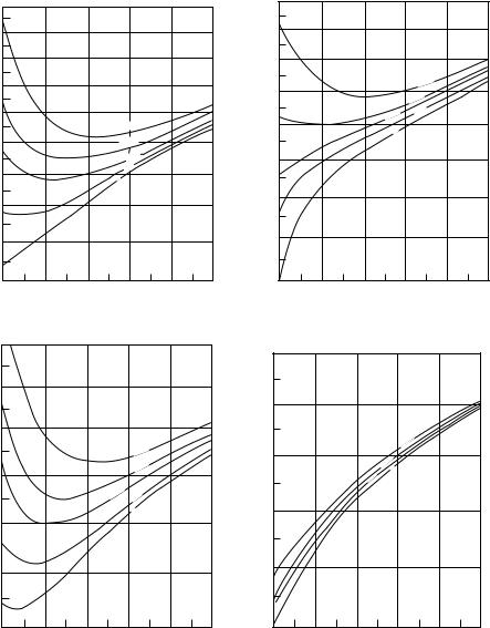

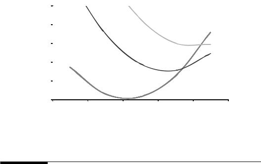
Appendix B: Tube-Side Heat Transfer Coefficients and Pressure Drop |
385 |
same as the number of streams. It can be a fraction or a multiple of the number of tubes wide. Some examples of superheater (and economizer) geometry are presented as follows to illustrate the concept of streams.
1.Superheater with horizontal tubes: In this case (Figure B.4a), we have a superheater in staggered arrangement. If there are, say, 30 tubes across the header in each row, then there are a total of 30 × 2 = 60 streams. Some engineers call the number of tubes in the same plane as starts. So there are 30 tubes across and 2 starts. The bottom line is that if 200,000 kg/h is the total flow of steam in this superheater, then 200,000/60 = 3,333 kg/h is the average flow per tube. This is w to be used in the
calculation of hc or P. Figure B.4a shows only four streams (2 × 2).
2.Vertical tube superheater: There are 18 tubes across, but by reviewing the header drawing (Figure B.4b), the plant engineer notices a baffle plate in the inlet header, and hence, there are nine streams only. The steam inlet and exit nozzles are on the same header. The other header is just a turnaround header, and so there is no baffle. Steam flows through nine tubes or nine streams in counter-flow direction and then makes a 180° turn and returns to the same header in parallel-flow fashion. This is done some-
times to lower the superheater tube wall temperatures (by increasing hc). Hence, if 27,000 kg/h is the total steam flow, the average flow per tube will be 3,000 kg/h.
3.Economizer (or superheater) with vertical tubes: In this drawing of a gas turbine HRSG economizer with vertical tubes (Figure B.4c), there are 12 tubes carrying water (across the width), but 24 tubes/row across the boiler width. All tubes are in counter-flow arrangement. Twenty-four tubes across are required from gas velocity considerations, but steam velocity consideration requires only half that number. This arrangement differs from that in Figure B.4b in that we have complete counter-flow in this case, while it is party counterand partly parallel-flow in earlier case. The LMTD values will accordingly be different and have to be evaluated. One may note that a collection header is required at the bottom for each row of tubes as there are incoming and outgoing tubes in each header. It is a more complicated arrangement to have streams as a third of the number of tubes wide. Hence, this arrangement is suitable for the number of streams half the number of tubes wide. If streams are the same as the number of tubes wide, then we can eliminate the collection header at the top of each row of tubes.
4.Economizer with low number of streams: In the case of Figure B.4d, there are eight tubes per row in the economizer with vertical downward gas flow, but the water flow requires only four streams. Hence, each tube is bent in the horizontal as well as in the vertical plane. Similarly, there can be 30 tubes across while streams can be 15 or 10 or 5 or even 6 or even 30 streams depending on water velocity required. Typically, 1–2 m/s is a good starting value for the velocity of water at 100% load. This arrangement is seen in gas turbines where the ratio of gas flow to steam flow is so large that the gas velocity demands a large number of tubes in the cross section while the water velocity requirement dictates a few tubes only. Figure shows eight tubes across with four streams. Note that in this type of arrangement, the transverse and longitudinal spacing are determined by the bend radius available for a given tube size.
5.Economizer or superheater with multiple streams: In this example of an economizer (Figure B.4e) or superheater, there are more streams than the tubes across. If the number of tubes wide is say 10, the streams are a multiple of it, 20. There can be 30 or even 60 streams depending on the ratio of gas to water flow. In a few waste

 View B
Appendix B: Tube-Side Heat Transfer Coefficients and Pressure Drop |
|
387 |
|
Gas in |
Water out |
|
|
|
|
|
|
|
Water in |
Out |
Water in |
|
out |
|
|
|
Water in |
(d) Gas out |
(e) |
|
Gas ow |
Superheater inlet
Superheater exit
(f)
Inlet
Outlet
(g) |
Gas ow |
FIGURE B.4 (Continued)
(d) Streams are a fraction of number of tubes wide. (e) Horizontal gas flow, horizontal tube superheater.
(f) Horizontal gas flow, horizontal tube superheater. (g) Counter-flow staggered finned tube economizer.
(Continued)

388 Appendix B: Tube-Side Heat Transfer Coefficients and Pressure Drop
From desuperheater |
|
Top header |
Sat steam |
|
Flue gas ow
Upper
|
|
+ SH header |
|
|
|
+ |
Lower |
|
Bottom header |
SH header |
|
|
|
||
|
+ |
|
|
|
|
|
|
To desuperheater |
|
Mud drum |
|
|
|
|
|
(h)Main steam outlet
Pass plate
 Gas ow
Coil layout
(i)side elevation
FIGURE B.4 (Continued)
(h) Vertical tube horizontal gas flow superheater. (i) Horizontal gas flow, horizontal tube economizer.

Appendix B: Tube-Side Heat Transfer Coefficients and Pressure Drop |
389 |
heat boilers, the flue gas flow will be quite small while the steam generation or water flowing in the economizer or condensate heater will be very large requiring multiple streams. Figure shows four streams (2 × 2).
6.Horizontal gas flow superheater with multiple tubes on each header: In this horizontal gas flow, horizontal tube superheater header (Figure B.4f), there are 2 tubes in each horizontal plane, and if there are 30 tubes along the header length, the number of streams is then 60. (Two starts on the header and 30 tubes across.) This could be arranged in parallelor counter-flow fashion depending on steam and tube wall temperatures. If there are four starts on the header, then the streams will be 30 × 4 = 120.
7.Vertical gas flow counter-flow economizer: In this counter-flow economizer (or superheater) (Figure B.4g), there are 20 tubes/row and 20 streams in staggered arrangement of tubes.
8.Inverted loop superheater: This is a common arrangement in package boilers (Figure B.4h). We have an inlet and exit header with multiple starts. The number of streams is decided based on steam velocity, pressure drop, tube wall temperature considerations, gravity versus friction loss at low loads, and height of the tubes. At the steam inlet, we have 6 starts with 5 tubes along the gas flow for a total of 30 streams. There is a baffle in the header after the 10th tube, so the 30 streams can reverse and flow up and down again. This is a commonly used arrangement in package boilers. The steam from the desuperheater has only 24 streams for illustration purposes. Here we have a baffle after the eighth row in the header.
Note that due to tube wall temperature limitations, the first stage is counterflow while the second stage is in parallel-flow. Thus, plant engineers should spend some time understanding their superheater flow configuration, which will help them evaluate its performance and those like this. As discussed in Chapter 3, at low loads, if the gravity loss in downward flow direction is larger than the steam pressure drop, then stagnation or reverse flow may occur. Hence, this is also a consideration for selecting the steam flow per tube or the number of streams.
9.Horizontal gas flow, horizontal tube economizer: In this economizer, the arrangement is uncommon (Figure B.4i). It has horizontal tubes and horizontal gas flow with a two-pass design! Sometimes due to layout considerations, this arrangement is warranted. There are 18 streams (9 × 2) in staggered arrangement. The water flows down from top-to-bottom header and then from bottom-to-top header. There is a baffle in the top header. Note that the total length along gas flow direction is small. We may have any number of such passes depending on the duty.
Pressure Drop inside Tubes
Pressure drop inside the tubes is also an important piece of information while designing superheaters, air heaters, economizers. Often, consideration of pressure drop and heat transfer coefficient determines the initial cost and cost of operation. Hence, pressure drop data along with the heat transfer coefficient help to optimize a design as will be shown in Chapter 2. The basic equation for pressure drop is
P = 810 × 10−6fLevw2/di5 |
(B.6) |
where P is the pressure drop in KPa (gas-steam-liquids).

390 |
Appendix B: Tube-Side Heat Transfer Coefficients and Pressure Drop |
Friction factor f varies with Reynolds number inside the tube and the tube roughness factor. Typically, flow in boilers, superheaters, economizers, and air heaters is turbulent, and hence, the friction factor is taken as a function of tube inner diameter as shown in Table B.5. Table B.6 shows the pressure drop equations in all systems of units.
TABLE B.5
Friction Factor as a Function of Tube Inner Diameter
Tube inner diameter (mm) |
19 |
25 |
38 |
51 |
63.5 |
76 |
101 |
126 |
200 |
250 |
Friction factor f |
0.0245 |
0.023 |
0.021 |
0.0195 |
0.018 |
0.0175 |
0.0165 |
0.016 |
0.014 |
0.013 |
Note: Standard pipe sizes are shown in Table B8.
TABLE B.6
Pressure Drop Equations
SI Units |
British Units |
Metric Units |
|
|
|
P = 810 × 10−6fLevw2/di5 |
P = 3.36 × 10⁻⁶fLevw2/di5 |
P = 0.6375 × 10⁻¹²fLevw2/di5 |
w, kg/s |
w, lb/h |
w, kg/h |
P, kPa |
P, psi |
P, kg/cm2 |
Le, m |
Le, ft |
Le, m |
v, m3/kg |
v, ft3/lb |
v, m3/kg |
di, m |
di, in. |
di, m |
P = 0.08262fLevw2/di5 |
P = 93 × 10−6fLevw2/di5 |
P = 6.382 × 10⁻⁹fLevw2/di5 |
P, mm wc in above equation |
P, in wc |
P, mm wc |
Notes: f = friction factor inside the tubes. Le = effective length of tube, m. One may use Table B.7 to determine the effective lengths in a coil or piping with bends and fittings. w = flow per tube = total flow of fluid/ streams, kg/s (if there are multiple streams, then based on effective length of each stream and tube diameter, flow and pressure drop equations must be solved to arrive at the flow in each stream. di = tube inner diameter, m. v = specific volume of fluid, m3/kg.
TABLE B.7
Effective Lengths for Bends, Valves, Fitting
Fitting |
Le/di |
90° square bend |
57 |
45° elbows |
15 |
90° elbows, standard radius |
32 |
90° elbows, medium radius |
26 |
90° elbows, long sweep |
20 |
180° elbows, close return bends |
75 |
180° medium radius return bends |
50 |
Gate valves open |
7 |
Gate valves, one-fourth closed |
40 |
Gate valves, half closed |
200 |
Gate valves, three-fourths closed |
800 |
Globe valves open |
300 |
|
|


392 |
Appendix B: Tube-Side Heat Transfer Coefficients and Pressure Drop |
References
1.P. Abbrecht and S. Churchill, The thermal entrance region in fully developed turbulent flow, AIChE Journal, 6, 268, June 1960.
2.V. Ganapathy, Applied Heat Transfer, Pennwell Books, Tulsa, OK, 1982, p600.
3.V. Ganapathy, Industrial Boilers and HRSGs, CRC Press, 2003, Boca Raton, FL, p531.


Appendix C: Heat Transfer Coefficients Outside Plain Tubes |
397 |
We can see that at 400°C, specific heat Cp = 0.289 kcal/kg °C (1210 J/kg K), viscosity µ = 0.1088 kg/m h (0.0000302 kg/m s), and thermal conductivity k = 0.0414 kcal/m h °C (0.0481 W/m K).
G = |
|
20 |
|
= 9.39 kg/m2 s (6,898 lb/ft2 h) |
|
|
|
||
|
12 × 3.5 × (0.1018 |
− 0.0508) |
|
|
Re = Gd/µ = 9.39 × 0.0508/0.0000302 = 15,795
Using Grimson’s correlation, B = 0.482, N = 0.556 for staggered, and B = 0.229, N = 0.632 for inline arrangement for ST/d = SL/d = 2.
For inline arrangement, Nu = 0.229 × 15,7950.632 = 103.1 or hc = 103.1 × 0.0481/.0508 = 97.6 W/m2 K (83.9 kcal/m2 h °C) (17.2 Btu/ft2 h °F).
For staggered arrangement, Nu = 0.482 × 15,7950.556 = 104 or hc = 98.56 W/m2 K (84.9 kcal/m2 h °C) (17.36 Btu/ft2 h °F).
Using Fishenden and Saunders equation,
Nu = 0.35 FhRe0.6Pr0.3
Re = 15,795
Pr = µCk p = 0.0000302 × 0.04811, 210 = 0.759
Fh for inline arrangement is 1.0, while for staggered, it is about 1.02.
Nu = 0.35 × 15,7950.6 × .7590.3 = 106.4 = hc × 0.0508 0.0481
or
hc = 100.8 W/m2 K (86.7 kcal/m2 h°C)(17.75 Btu/ft2 h°F)
hc is about 2% more for staggered arrangement.
Hence, it may be seen that the difference in hc between staggered and inline arrangements is not significant. Hence, gas pressure drop over plain tubes should be estimated to see which arrangement is better. Gas pressure drop gives an idea of the incremental addition to the fan power consumption. This is discussed later.
Variation of Convective Heat Transfer Coefficients around Tube Periphery
The correlations discussed earlier for heat transfer provide an estimate for the average value of hc for the tube bundle. hc varies around the tube periphery and also along the tube rows as shown in Figure C.3a through c. Figure C.3b is for inline, while Figure C.3c is for staggered arrangement. While determining the maximum tube wall temperature for selecting materials for a superheater, which operates at high gas temperature, one should estimate the maximum value of hc in a given tube row. The maximum value of hc occurs at the tube front and decreases to a minimum at about 90° and again increases to a maximum at 180°. The ratio of hc′/hc, the ratio of local heat transfer coefficient to

398 |
Appendix C: Heat Transfer Coefficients Outside Plain Tubes |
Direction |
Pipe |
|
of stream |
||
|
|
|
(a) |
|
|
|
|
|
|
2.0 |
|
hc΄/hc |
|
2.0 |
|
hc΄/hc |
|
|
1.8 |
|
2 |
|
1.8 |
|
|
|
|
1.6 |
|
|
|
|
|
|
|
|
|
1 |
180° |
1.6 |
|
2 |
0° |
180° |
|
1.4 |
|
0° |
1.4 |
|
|
|||
3–7 |
|
|
3–7 |
|
|
|||
1.2 |
|
|
|
1.2 |
|
|
|
|
|
|
90° |
|
|
1 |
|
||
1.0 |
|
|
1.0 |
|
|
90° |
||
|
|
|
|
|
||||
0.8 |
|
|
3–7 |
0.8 |
|
|
|
3–7 |
|
|
|
|
|
|
|||
0.6 |
|
|
2 |
0.6 |
|
|
|
2 |
0.4 |
|
|
1 |
0.4 |
|
|
|
|
|
|
|
|
|
|
|||
|
|
|
|
|
|
1 |
||
0.2 |
|
|
|
0.2 |
|
|
|
|
|
|
|
|
|
|
|
||
0 |
0 |
30 60 90 |
120 150 deg |
0 |
0 |
30 60 90 |
120 150 deg |
|
(b) |
|
Inline |
|
(c) |
|
|
Staggered |
|
FIGURE C.3
Variation of heat transfer coefficient around tube periphery. The numbers 1–7 (in b and c) refer to row along gas flow.
the average, depends on the Reynolds number and tube arrangement, whether inline or staggered. It can be seen that the second tube shows a maxima larger than the first for inline arrangement (Figure C.3b). In staggered arrangement, a similar effect is seen (Figure C.3c) but at a different point in the periphery. In inline arrangement, hc′ can be 1.6 times the average hc in row 1, while in row 2, it is about 1.7. Beyond two rows, hc’ is about 1.4 times the average value. Hence, for estimating tube wall temperature and selecting materials in counter-flow arrangements, the first two to three rows assume significance.
Though the figures stress the fact that there is variation in heat transfer coefficient around the tube periphery and along the gas flow direction, it is better to do actual tube wall temperature measurements in the first few rows of high temperature surface such as a superheater and confirm the correction factors or correlate it with the calculated tube wall temperatures. This will help the engineer select appropriate materials for these critical heating surfaces. The charts provided earlier show results from limited tests and are shown for informative purposes.

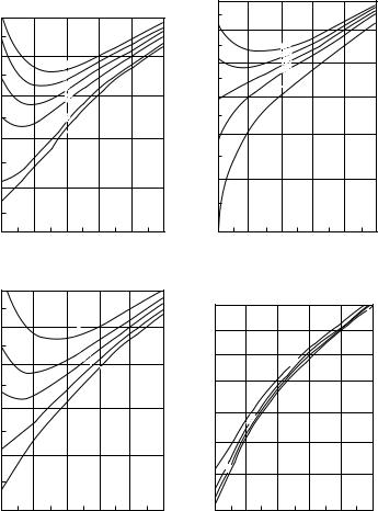


Appendix C: Heat Transfer Coefficients Outside Plain Tubes |
401 |
For staggered arrangement, f = 15,795−0.16[0.25 + 0.1175/1] = 0.078 Hence, gas pressure drop will be 0.078/0.0478 × 20 = 33 mm wc
Hence, for nearly the same heat transfer coefficient or size of tube bundle, the gas pressure drop is about 60% higher, which means more operating cost. Hence, inline arrangement of plain tubes is generally preferred over staggered arrangement in boiler practice for plain tubes.
Effect of Gas Pressure on Heat Transfer
The effect of gas pressure is similar to that of flow inside tubes. Figure C.4 shows results for common gases. The effect is not significant till 40 bar pressure, and hence, for boiler, heater, or HRSG applications, the effect of gas pressure may be neglected.
Effect of Tube Size on Boiler Design
It may be shown that when small-diameter tubes are used in the boiler for the same gas pressure drop and duty, the smaller-diameter option will have lower weight and hence easier handling and lower shipping costs. However, the number of tubes to be welded to the headers (or drums) will be more, increasing the cost of labor. One also has to check the cost of materials including the cost of longer drums or headers. In any event, effect of tube size on heat transfer must be understood by plant engineers as different boiler suppliers around the world may come up with boiler designs with different tube sizes, and an idea of how this affects the size, surface area, and weight is important while evaluating the designs. It is the author’s view that in locations where labor costs are low and material costs are high, smaller-diameter tubes may be used.
Example C.3
Flue gases of 200,000 kg/h from natural gas products of combustion has to be cooled from 600°C to 311°C in a bare tube boiler generating saturated steam at 40 kg/cm2 a (saturated steam temperature = 249°C). Tubes measuring 50.8 mm and 38 mm are available. For the same gas pressure drop, determine which option weighs less. Flue gas analysis % volume CO2 = 8, H2O = 18, N2 = 71, O2 = 3. Use inline arrangement. Fouling factors are 0.0002 m2 h °C/kcal for both gas and steam. (Assume boiling heat transfer coefficient as 12250 kcal/m2hoC.)
Let us use 50.8 × 43 mm plain tubes 24 tubes/row, 8 m long with transverse and longitudinal pitch = 78 mm. For the 38 mm tubes, use a rectangular spacing of 66 mm. The number of rows deep has to be estimated from Uo, the overall heat transfer coefficient.
Let us determine the convective heat transfer coefficient. Gas properties at average film temperature have to be obtained. The tube wall temperature will be close to that of steam temperature due to the high boiling heat transfer coefficient. Hence, let us assume that tube outer wall temperature = 260°C. Average gas temperature is (600 + 311)/2 = 455°C. Average film temperature = (455 + 260)/2 = 357°C.
From Appendix F at film temperature of 357°C, Cp = 0.2860 kcal/kg °C, µ = 0.1038 kg/m h, k = 0.03925 kcal/m h °C. At an average gas temperature of 455°C, Cp = 0.2924, µ = 0.1143 kg/m h, k = 0.04395 kcal/m h°C.
402 |
Appendix C: Heat Transfer Coefficients Outside Plain Tubes |
Gas mass velocity G = 200,000/[24 × 8 × (0.078 − 0.0508)] = 38,297 kg/m2 h
Re = Gd/µ = 38,297 × 0.0508/0.1038 = 19,232. Use Grimson’s correlations. Obtain factors B and N from Table C.2. B = 0.25 N = 0.62
Nu = 0.25 × 192320.62 = 113.2 = hc × 0.0508/0.0.03925 or hc = 87.46 kcal/m2 h °C (17.85 Btu/ ft2 h °F). (We may also obtain hc in W/m2 K using appropriate properties as done earlier. Let us not use any correction factors as the purpose is to see the effect of tube size only.)
Nonluminous Heat Transfer Coefficient hn (See Appendix D)
Beam length L = 1.08 × (0.078 × 0.078 − 0.785 × 0.0508 × 0.0508)/0.0508 = 0.086 m
|
|
K |
= (0.8 + 1.8 × 0.18) × (1 − 0.38 × 0.728) × |
|
(0.08 + 0.18) |
= 1.413 |
|
|
|
|
|||||||||||||
|
|
(0.26 × 0.086)0.5 |
|
|
|
|
|||||||||||||||||
|
|
|
|
|
|
|
|
|
|
|
|
|
|
|
|
|
|
|
|||||
|
|
|
|
|
Gas emissivity g = 0.9 × (1 − e−1.413 × 0.086) = 0.102 |
|
|
|
|
|
|
||||||||||||
|
hn |
= 5.67 |
10−8 0.102 |
(7.28 |
4 |
− 5.33 |
4 |
) = 5.93 W/m2 K = 5.1 kcal/m2h°C |
|
|
|||||||||||||
|
|
|
|
|
|
|
|
|
|
|
|
|
|
|
|
|
|
|
|
|
|||
|
|
|
|
|
|
(728 − 533) |
|
|
|
|
|
|
|
|
|
|
|
|
|||||
|
|
1 |
|
|
|
|
50.8 |
|
|
1 |
|
|
0.0508 |
|
0.0508/2 |
|
|
50.8 |
|||||
Uo = |
|
|
|
|
+ 0.0002 + 0.0002 |
|
+ |
|
|
|
|
|
+ |
|
|
|
ln |
|
|
||||
(5.1 |
+ 87.46) |
|
12,250 |
043 |
37 |
43 |
|||||||||||||||||
|
|
|
43 |
|
|
|
|
|
|
|
|
|
|||||||||||
= 0.01144 |
|
or Uo = 87.36 kcal/m2h°C(17.83 Btu/ft2h°F) |
|
|
|
|
|
|
|
||||||||||||||
Duty = 200,000 × .99 × (600 − 311) × 0.2924 = 16.73 × 10⁶ kcal/h (use a heat loss of 1%)
LMTD = (600 − 311)/[(600 − 249)/(311 − 249)] = 167°C. Surface area required = 16.73 × 10⁶/167/87.36 = 1151 m2 = 3.14 × 0.0508 × 24 × 8 × Nd, where Nd is the number of rows deep. Nd = 37.5. 38 rows were used as headers have to be brought to the same side of the bundle.
Gas Pressure Drop
Pg = 0.204 f G2Nd/ρg
Reynolds number for pressure drop is computed at the average gas temperature. Re = 38,297 × 0.0508/0.1143 = 17,020. ρg at average gas temperature of 455°C = (27.6/22.4) × 273/ (273 + 455) = 0.4614 kg/m3 (MW of flue gas = 27.6).
|
−0.15 |
|
|
|
0.08 SL/d |
|
|
|
||||
f = Re |
|
0.044 + |
|
|
|
|
|
|
|
= 0.0693 |
||
|
|
|
(0.43 |
|
|
|
||||||
|
|
|
|
|
|
+ 1.13 d/ST ) |
|
|||||
|
|
|
|
(ST/d − 1) |
|
|
|
|
|
|||
Pg = 0.204 0.0693 |
|
|
38, 297 |
2 |
38 |
|
|
132 mm wc |
||||
|
|
|
|
|
= |
|||||||
3,600 |
0.4614 |
|||||||||||
|
|
|
|
|
|
|
|
|
||||
Similar calculations may be done for the 38 mm tubes. Results are shown in Table C.6. It can be seen that the overall heat transfer coefficient is higher with the smaller tube. It may be also noted that the weight of the 38 mm tube design is lower for the same gas pressure drop and duty. However, this has to be balanced by the cost of manufacturing as we have
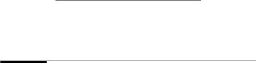
Appendix C: Heat Transfer Coefficients Outside Plain Tubes |
403 |
|||
|
TABLE C.6 |
|
|
|
|
Comparison of 50.8 and 38 mm Tubes |
|
|
|
|
|
|
|
|
|
Item |
50.8 mm |
38 mm |
|
|
|
|
|
|
|
Gas flow, kg/h |
200,000 |
200,000 |
|
|
Gas inlet temp., °C |
600 |
600 |
|
|
Gas exit temp., °C |
311 |
311 |
|
|
Duty, MM kcal/h |
16.7 |
16.9 |
|
|
Gas press. drop, mm wc |
132 |
130 |
|
|
Tubes/row |
24 |
24 |
|
|
Length, m |
8 |
8 |
|
|
No. of rows deep |
38 |
47 |
|
|
Transverse pitch, mm |
78 |
66 |
|
|
Longitudinal pitch, mm |
78 |
66 |
|
|
U , kcal/m2 h °C |
86.8 |
94.0 |
|
|
o |
|
|
|
|
Surface area, m2 |
1,160 |
1,074 |
|
|
Weight, kg |
34,310 |
25,840 |
|
Note: Large longitudinal spacing is not recommended.
more tubes to be welded or rolled on to the drums or headers. Hence, one may review options with smaller-diameter tubes if weight of the boiler is a concern. As mentioned earlier, the cost of fabrication may differ depending on local manufacturing costs.
Effect of Longitudinal Spacing
With plain tubes, the longitudinal spacing in inline arrangement impacts the gas pressure drop significantly while contributing slightly to the overall heat transfer coefficient. Tube spacing is generally based on tube bend radius available for a given tube size and ligament efficiency in boiler drums and also on the boiler manufacturer’s practice. However, choosing a large longitudinal spacing increases the gas pressure drop and thus increases the operating cost. The nonluminous heat transfer coefficient is increased due to the increase in beam length. It also increases the drum or header lengths and increases the cost of the boiler.
Example C.4
Flue gases of 100,000 kg/h in a boiler are cooled from 700°C to 326°C. Flue gas analysis is % volume CO2 = 8, H2O = 18, N2 = 71, O2 = 3. Tubes are 50.8 mm OD × 43 mm. Steam is generated at 40 kg/am2 a.Compare the design with a transverse tube spacing of 76 mm with longitudinal spacing of 76,101 and 152 mm, respectively, in inline arrangement.
Using Grimson’s correlations, calculations were performed using a computer program, and the results are presented in Table C.7. While the convective heat transfer coefficient changes within 1%, the nonluminous coefficient increases due to the higher beam length (see Appendix D). Hence, Uo values are slightly higher when SL increases. However, the gas pressure drop increases much more, by about 40% when SL/d = 3 compared to when SL/d = 1.5.
So the boiler designer should consider using smaller bend radius while fabricating the bundle or a smaller longitudinal pitch, while the plant engineer should be aware of the implications of SL.
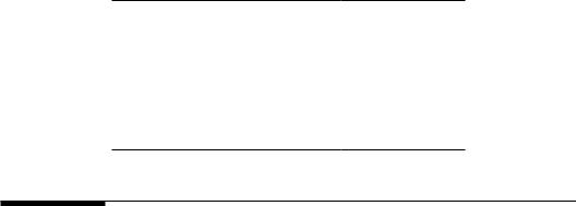
Appendix C: Heat Transfer Coefficients Outside Plain Tubes |
405 |
|||||
Substituting for G from (C.8a), we have |
|
|||||
|
Q |
= UA = 1.044 F2Wg0.6NwNdL |
(C.11) |
|||
|
|
|||||
|
T |
N0.6w L0.6 (ST/d − 1)0.6 |
|
|||
= |
1.044F2Wg0.6Nw0.4L0.4Nd |
|
(C.12) |
|||
(ST/d − 1)0.6 |
||||||
|
|
|
|
|||
This equation may be used to relate the tube geometry with duty. However, when there is a phase change as in a boiler evaporator, the equation may be simplified further.
ln [(T1 − Ts)/(T2 − Ts)] = UA/(WgCp) (as seen in Appendix A) |
|
||||||
= |
1.044F2Wg0.6Nw0.4L0.4Nd/(ST/d − 1)0.6 |
|
|||||
|
|
|
(WgCp ) |
|
|||
= |
1.044F2N0w.4L0.4Nd (ST/d − 1)0.6 |
|
|||||
|
|
|
(Wg0.4Cp ) |
|
|||
= |
1.044(F2/Cp )Nd |
|
|
(C.13a) |
|||
G |
0.4 |
(ST/d − 1)d |
0.4 |
|
|||
|
|
|
|
|
|||
If the tube geometry is known, one can estimate Nd or G for a specific thermal performance. Now introducing the equation for gas pressure drop (inline which is widely used),
Pg = |
0.204 f G2Nd (if G is in kg/m2s) |
|
or |
Pg = 1.574 × 10⁻⁸ f G2Nd |
(G in kg/m2h) |
|||||||||||||||
|
ρg |
|
|
|
|
|
|
|
|
|
|
|
ρg |
|
|
|
|
(C.13b) |
||
|
|
|
|
f = Re−0.15X |
|
|
|
|
|
|
|
|
|
|
(C.13c) |
|||||
where |
|
|
|
|
|
|
|
|
|
|
|
|
|
|
|
|
|
|
|
|
|
X = 0.044 |
+ |
|
|
|
0.08SL/d |
|
|
|
|
|
|
|
|
||||||
|
(ST/d − 1)(0.43+1.13d/SL ) |
|
|
|
|
|
|
|||||||||||||
Substituting for Re = Gd/µ in above equation C.13c and for Nd from (C.13), we have |
|
|||||||||||||||||||
|
|
−8 |
|
|
|
2.25 |
|
(T1 |
− Ts ) |
|
(ST − d)X |
|
||||||||
|
Pg = 1.5077 10 |
|
G |
|
|
ln |
|
|
|
|
|
|
|
|
|
|
|
(C.14) |
||
|
|
|
|
(T2 |
|
|
|
0.75ρ |
|
|
||||||||||
|
|
|
|
|
|
|
|
|
− Ts ) |
|
|
|
||||||||
|
|
|
|
|
|
|
|
|
|
|
|
|
|
F3d |
|
g |
|
|||
where |
|
|
|
|
|
|
|
|
|
|
|
|
|
|
|
|
|
|
|
|
|
|
|
F3 = |
|
k0.7 |
|
|
|
|
|
|
|
|
|
|
|
(C.15) |
|||
|
|
|
(Cp0.7µ0.45 ) |
|
|
|
|
|
|
|
|
|||||||||
This is a very important equation linking gas pressure drop with thermal performance and duty. While a computer program would yield close results, equations such as this help one visualize the impact of variables on boiler design and performance.

408 |
Appendix D: Nonluminous Heat Transfer Calculations |
|||||
In British units, |
|
|
|
|
|
|
|
|
4 |
4 |
|
|
|
|
hn = |
σg Tg |
– To |
|
|
(D.4b) |
|
(Tg − To ) |
|
||||
where
σ is the Steffan–Boltzman constant = 0.1714 × 10⁻⁸
Tg, To in °R
hn in Btu/ft2 h °F
To estimate hn, partial pressures of triatomic gases and beam length L are required. L is a characteristic dimension that depends on the bundle arrangement and shape of enclosure.
For a plain tube bundle,
L = |
1.08 |
× (STSL |
− 0.785d2 ) |
† |
(D.5) |
|
d |
|
|||
|
|
|
|
|
For a cavity, L is approximately 3.4–3.6 times the volume of the space divided by the surface area of the heat-receiving surface. If a, b, c are the dimensions of the cavity,
L = |
3.4abc |
= |
1.7 |
(D.6) |
2(ab + bc + ca) |
(1/a + 1/b + 1/c) |
For flow inside tubes, the tube inner diameter may be taken as L. As di is generally small, the beam length and hence the emissivity is small, and hn inside tubes may be neglected if the convective coefficient is large.
For a finned tube bundle,
|
(ST SL ) |
|
|
|
Beam length Lb = (d + 2h) |
|
|
− 0.85 |
(D.7) |
(d + 2h) |
2 |
|||
|
|
|
|
|
Example D.1
Estimate the beam length when 50.8 mm tubes in a boiler bank are arranged with a transverse pitch of 101 mm and longitudinal pitch of 127 mm.
Solution
L = 1.08 × (0.1018 × 0.127 − 0.785 × 0.0508 × 0.0508)/0.0508 = 0.23 m
Example D.2
Flue gases with CO2 = 12% and H2O = 16% by volume are flowing across a superheater tube bundle. If 50.8 mm tubes are arranged with ST = 101 mm and SL = 127 mm, determine hn. Flue gas pressure is atmospheric. Average gas temperature Tg = 900°C and average wall temperature To = 300°C.

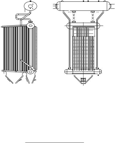
Appendix D: Nonluminous Heat Transfer Calculations |
411 |
||||||||||||||||||||||||||||||||||||||||||||||||||||||||
|
|
|
|
|
|
|
|
|
|
|
|
|
|
|
|
|
|
|
|
|
|
|
|
|
|
|
|
|
|
|
|
|
|
|
|
|
|
|
|
|
|
|
|
|
|
|
|
|
|
|
|
|
|
|
|
|
|
|
|
|
|
|
|
|
|
|
|
|
|
|
|
|
|
|
|
|
|
|
|
|
|
|
|
|
|
|
|
|
|
|
|
|
|
|
|
|
|
|
|
|
|
|
|
|
|
|
|
|
|
|
|
|
|
|
|
|
|
|
|
|
|
|
|
|
|
|
|
|
|
|
|
|
|
|
|
|
|
|
|
|
|
|
|
|
|
|
|
|
|
|
|
|
|
|
|
|
|
|
|
|
|
|
|
|
|
|
|
|
|
|
|
|
|
|
|
|
|
|
|
|
|
|
|
|
|
|
|
|
|
|
|
|
|
|
|
|
|
|
|
|
|
|
|
|
|
|
|
|
|
|
|
|
|
|
|
|
|
|
|
|
|
|
|
|
|
|
|
|
|
|
|
|
|
|
|
|
|
|
|
|
|
|
|
|
|
|
|
|
|
|
|
|
|
|
|
|
|
|
|
|
|
|
|
|
|
|
|
|
|
|
|
|
|
|
|
|
|
|
|
|
|
|
|
|
|
|
|
|
|
|
|
|
|
|
|
|
|
|
|
|
|
|
|
|
|
|
|
|
|
|
|
|
|
|
|
|
|
|
|
|
|
|
|
|
|
|
|
|
|
|
|
|
|
|
|
|
|
|
|
|
|
|
|
|
|
|
|
|
|
|
|
|
|
|
|
|
|
|
|
|
|
|
|
|
|
|
|
|
|
|
|
|
|
|
|
|
|
|
|
|
|
|
|
|
|
|
|
|
|
|
|
|
|
|
|
|
|
|
|
|
|
|
|
|
|
|
|
|
|
|
|
|
|
|
|
|
|
|
|
|
|
|
|
|
|
|
|
|
|
|
|
|
|
|
|
|
|
|
|
|
|
|
|
|
|
|
|
|
|
|
|
|
|
|
|
|
|
|
|
|
|
|
|
|
|
|
|
|
|
|
|
|
|
|
|
|
|
|
|
|
|
|
|
|
|
|
|
|
|
|
|
|
|
|
|
|
|
|
|
|
|
|
|
|
|
|
|
|
|
|
|
|
|
|
|
|
|
|
|
|
|
|
|
|
|
|
|
|
|
|
|
|
|
|
|
|
|
|
|
|
|
|
|
|
|
|
|
|
|
|
|
|
|
|
|
|
|
|
|
|
|
|
|
|
|
|
|
|
|
|
|
|
|
|
|
|
|
|
|
|
|
|
|
|
|
|
|
|
|
|
|
|
|
|
|
|
|
|
|
|
|
|
|
|
|
|
|
|
|
|
|
|
|
|
|
|
|
|
|
|
|
|
|
|
|
|
|
|
|
|
|
|
|
|
|
|
|
|
|
|
|
|
|
|
|
|
|
|
|
|
|
|
|
|
|
|
|
|
|
|
|
|
|
|
|
|
|
|
|
|
|
|
|
|
|
|
|
|
|
|
|
|
|
|
|
|
|
|
|
|
|
|
|
|
|
|
|
|
|
|
|
|
|
|
|
|
|
|
|
|
|
|
|
|
|
|
|
|
|
|
|
|
|
|
|
|
|
|
|
|
|
|
|
|
|
|
|
|
|
|
|
|
|
|
|
|
|
|
|
|
|
|
|
|
|
|
|
|
|
|
|
|
|
|
|
|
|
|
|
|
|
|
|
|
|
|
|
|
|
|
|
|
|
|
|
|
|
|
|
|
|
|
|
|
|
|
|
|
|
|
|
|
|
|
|
|
|
|
|
|
|
|
|
|
|
|
|
|
|
|
|
|
|
|
|
|
|
|
|
|
|
|
|
|
|
|
|
|
|
|
|
|
|
|
|
|
|
|
|
|
|
|
|
|
|
|
|
|
|
|
|
|
|
|
|
|
|
|
|
|
|
|
|
|
|
|
|
|
|
|
|
|
|
|
|
|
|
|
|
|
|
|
|
|
|
|
|
|
|
|
|
|
|
|
|
|
|
|
|
|
|
|
|
|
|
|
|
|
|
|
|
|
|
|
|
|
|
|
|
|
|
|
|
|
|
|
|
|
|
|
|
|
|
|
|
|
|
|
|
|
|
|
|
|
|
|
|
|
|
|
|
|
|
|
|
|
|
|
|
|
|
|
|
|
|
|
|
|
|
|
|
|
|
|
|
|
|
|
|
|
|
|
|
|
|
|
|
|
|
|
|
|
|
|
|
|
|
|
|
|
|
|
|
|
|
|
|
|
|
|
|
|
|
|
|
|
|
|
|
|
|
|
|
|
|
|
|
|
|
|
|
|
|
|
|
|
|
|
|
|
|
|
|
|
|
|
|
|
|
|
|
|
|
|
|
|
|
|
|
|
|
|
|
|
|
|
|
|
|
|
|
|
|
|
|
|
|
|
|
|
|
|
|
|
|
|
|
|
|
|
|
|
|
|
|
|
|
|
|
|
|
|
|
|
|
|
|
|
|
|
|
|
|
|
|
|
|
|
|
|
|
|
|
|
|
|
|
|
|
|
|
|
|
|
|
|
|
|
|
|
|
|
|
|
|
|
|
|
|
|
|
|
|
|
|
|
|
|
|
|
|
|
|
|
|
|
|
|
|
|
|
|
|
|
|
|
|
|
|
|
|
|
|
|
|
|
|
|
|
|
|
|
|
|
|
|
|
|
|
|
|
|
|
|
|
|
|
|
|
|
|
|
|
|
|
|
|
|
|
|
|
|
|
|
|
|
|
|
|
|
|
|
|
|
|
|
|
|
|
|
|
|
|
|
|
|
|
|
|
|
|
|
|
|
|
|
|
|
|
|
|
|
|
|
|
|
|
|
|
|
|
|
|
|
|
|
|
|
|
|
|
|
|
|
|
|
|
|
|
|
|
|
|
|
|
|
|
|
|
|
|
|
|
|
|
|
|
|
|
|
|
|
|
|
|
|
|
|
|
|
|
|
|
|
|
|
|
|
|
|
|
|
|
|
|
|
|
|
|
|
|
|
|
|
|
|
|
|
|
|
|
|
|
|
|
|
|
|
|
|
|
|
|
|
|
|
|
|
|
|
|
|
|
|
|
|
|
|
|
|
|
|
|
|
|
|
|
|
|
|
|
|
|
|
|
|
|
|
|
|
|
|
|
|
|
|
|
|
|
|
|
|
|
|
|
|
|
|
|
|
|
|
|
|
|
|
|
|
|
|
|
|
|
|
|
|
|
|
|
|
|
|
|
|
|
|
|
|
|
|
|
|
|
|
|
|
|
|
|
|
|
|
|
|
|
|
|
|
|
|
|
|
|
|
|
|
|
|
|
|
|
|
|
|
|
|
|
|
|
|
|
|
|
|
|
|
|
|
|
|
|
|
|
|
|
|
|
|
|
|
|
|
|
|
|
|
|
|
|
|
|
|
|
|
|
|
|
|
|
|
|
|
|
|
|
|
|
|
|
|
|
|
|
|
|
|
|
|
|
|
|
|
|
|
|
|
|
|
|
|
|
|
|
|
|
|
|
|
|
|
|
|
|
|
|
|
|
|
|
|
|
|
|
|
|
|
|
|
|
|
|
|
|
|
|
|
|
|
|
|
|
|
|
|
|
|
|
|
|
|
|
|
|
FIGURE D.2
Waste heat boiler with furnace section.
Solution
Assume the exit gas temperature of 800°C = 1073 K. Use saturation temperature plus 18°C for tube outer wall temperature = 220°C = 493 K. Average specific heat of the gas is 1323 J/kg K between 1000°C and 800°C.
At 900°C = 1173 K average gas temperature, the emissivity of the flue gases may be computed.
The beam length of the furnace is 1.7/(1/3 + 1/4 + 1/8) = 2.41 m
K = (0.8 + 1.6 × .15)(1 − .00038 × 1173)× 0.27 = 0.193 (0.27 × 2.41)0.5
Gas emissivity = 0.9 × (1 − e−0.193 × 2.41) = 0.334
Hence, radiation to furnace walls = 136 × 0.334 × 0.9 × 5.67 × 10−8 × (11734 − 4934) = 4,251 kW Energy from flue gases = 27.8 × 1323 × (1,000 − 800) × .99 = 7,282,300 W = 7,282 kW
So the assumed exit gas temperature is too low.
Try exit gas temperature = 900°C or average gas temperature = 950°C = 1,223 K Gas emissivity = (0.8 + 1.6 × 0.15) × (1 − 0.00038 × 1223) × 0.27/(0.27 × 2.41)0.5 = 0.186 Gas emissivity = 0.9 × (1 − e−0.186 × 2.41) = 0.325
Hence, radiation to furnace walls = 0.325 × 0.9 × 5.67 × 10−8 × (12234 − 4934) × 136 = 4912 kW Energy from flue gases = 27.8 × 1,323 × (1,000 − 900) = 7,355,880 W = 3,677 kW
Try exit gas temperature = 870°C average gas temperature = 935°C = 1,208 K Using the same emissivity,
Radiation to furnace = 0.325 × 0.9 × 5.67 × 10−8 × (12084 − 4944) × 136 = 4,668 kW Energy from flue gases = 27.8 × 1323 × 130 × 0.99 = 4,733 kW.
Hence, flue gas exit temperature is approximately 870°C. With a computer program, one can study the effect of varying the furnace dimensions on the furnace duty and exit gas temperature. For improved accuracy, one may split up the furnace into zones and arrive at the exit gas temperature and duty more accurately.

412 |
Appendix D: Nonluminous Heat Transfer Calculations |
Large Tube Spacing Increases hn
In boiler practice, some manufacturers use a large longitudinal spacing due to considerations such as availability of tube bends, manufacturing practice, and drum ligament efficiency. Transverse tube pitch impacts gas velocity and pressure drop, while longitudinal pitch increases the beam length and hence hn. Longitudinal pitch in plain tubes also increases the gas-side pressure drop as shown in Appendix C and hence should be avoided.
Example D.5
A tube bundle uses an ST/d of 1.5 and SL/d of 1.5 and 3. What is the impact on hn at 700°C gas temperature? Pc = 0.08, Pw = 0.18 and d = 50.8 mm.
Beam length L when ST/d = 1.5, SL/d = 1.5 is 1.08 × (1.5 × 1.5 − 0.785) × 0.0508 = 0.08 m
K = (0.8 + 1.8 × 0.18) × (1 − 0.00038 × 973) × 0.26/(0.26 × 0.08)0.5 = 1.236
g = 0.9 × (1 − e−1.236 × 0.08) = 0.085
Similarly, when SL/d = 3, L = 0.204 m, K = 0.774, and g = 0.131. Hence, gas emissivity increases, which increases hn.
However, as shown in Appendix C, the gas pressure drop increases significantly as SL/d increases, and hence, this is not a good design practice. Use as small an SL/d as possible. This will also conserve space and reduce the length of the bundle, drums, and hence cost of boiler. Using a large SL increases the U and heat flux and the tube wall temperature. Effect of SL is also discussed in Appendix C, Example C.4.
Example D.6
In a fire tube boiler, the average gas temperature of flue gases inside the tubes is 537°C (810 K) and tube inner diameter is 45 mm. Tube wall temperature is about 195°C (468 K). Pc = Pw = 0.12. Flue gas is at atmospheric pressure. Estimate hn.
The beam length of the tube ID = 0.045 m
K = (0.8 + 1.6 × 0.12)× (1 − 0.00038 × 810)× 0.24 = 1.586 (0.24 × 0.045)0.5
g = 0.9(1 − e−1.586 × 0.045) = 0.062
hn = 5.67 × 10−8 × 0.062 × (8104 − 4684 ) = 3.93 W/m2K (810 − 468)
hn inside fire tube boilers is usually small and neglected as the beam length is small.
Bibliography
1.W. Roshenow, J.P., Hartnett, Handbook of Heat Transfer, McGraw-Hill, New York, 1972.
2.V. Ganapathy, Applied Heat Transfer, Pennwelll Books, Tulsa, OK, 1982.