Учебное пособие 2092

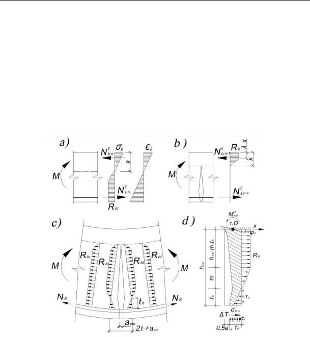
T is shearing forces at concrete-reinforcement contact area, P1, P2 are the result of compressive and tensile forces along the height of a two-console element respectively, q is uniform load along the height of the two-console element at the moment of crack formation equal to σbt * b, Mcon is a fixed end moment in a two-console element.

When hcrc = 0, the shear force T = Gτεqelbt, where hcrc is a crack length, Gτ is a concretereinforcement mutual displacement modulus, εqel is a relative mutual displacement of concrete and reinforcement at length t.

Internal forces Nbt in the area adjacent to a crack in a reinforced concrete bar at the moment of crack formation can be calculated on the basis of a two-console element [11, 18]:

b is the width of a reinforced concrete element; σS·AS is the tensile force in rebars at load

P = λcrcq; σSP·ASP is a pre-tensioning force; t = 1,5·d is a parameter characterizing a dimension of the compressed concrete near crack (d is the diameter of main reinforcement); hcrc = h0 –

– d/2 – xcrc is the crack length; xcrc = ξ·h0 is the height of the compressed area of concrete in reinforced concrete element in bending at the moment of crack formation; ∆Т are shear forces in con- crete-reinforcement contact area; m is a pre-failure zone; kbr is a critical stress intensity factor.

The design stress σbt,c at concrete-reinforcement contact area and shear force increment ∆Т

(see Fig. 2, d) in the first step of iteration can be defined as follows:

The possible area of В4 change can be determined within the following limits:

0 B4 e B tb . (13)

If В4 < 0, then lnB4 that corresponds to the condition before crack formation does not exist (acrc = 0).

If B4 = eB·tb, then the distance between crack that corresponds to the condition when the distance between cracks is so small that the bond between concrete and reinforcement is equal to zero and is thus negligible.

11

Scientific Herald of the Voronezh State University of Architecture and Civil Engineering. Construction and Architecture

If the condition (13) is not satisfied on the right, then the level of stresses σbt,c and forced ∆Т should be decreased.

The functional value of the distance between cracks lcrc can be defined as follows:

Shear and normal stresses (τb(z) and σp) in rebars shown in Fig. 2, are not included in equilibrium equation since their projection on x-axis is equal to zero and in moment equilibrium equation their arms are negligible. The dowel action of rebars is not considered either.

Fig. 2. Analytical schemes of reinforced concrete element in bending for additional dynamic stress calculation: cross-section without cracks (a), cross-section with cracks (b); cross-section at the moment of crack formation (c); a model of two-console element (d)

Calculation of stresses in rebars for n-times in a statically indeterminate system (with-

out cracks). Stage Ia of stress-strain state. Concrete stresses σbt approach the limit tensile stress Rbt. Non-elastic strain develops in the tensile Nb + Nbt + N S,c n = 0 area of concrete,

concrete stress diagram at a tension area becomes curved and deformations approach the limit values. A compressed area of concrete is mainly under elastic strain. Concrete stress diagram at a compression area is close to a triangular shape (see Fig. 2, a).

12

The internal force in rebars for the considered stage can be deduced from the equation of force equilibrium along x-axis (∑X = 0):

Nb and NS –– are respectively longitudinal internal forces of concrete and rebars in tension in the static state.

Nb can be deduced from the equation of an equilibrium moment of about 0 point (∑M = 0):

Calculation of stresses in rebars for n-times in a statically indeterminate system (with cracks). Stage II of stress-strain. In a tension area at cross-section with crack tension forces are taken by rebars and concrete in tension above cracks. In the zones between cracks the concrete-reinforcement bond mainly remains and concrete works under tension. Further on, as load increases, the crack reaches the neutral line and opens up, therefore the whole tension is taken on by rebars (see Fig. 2,b). The internal force in rebars for considered stage can be expressed from the equation of force equilibrium along x-axis (∑X = 0):

Nb + NS + Nbt = 0 ; N S = Nb Nbt ,

Nb can be expressed from the equation of moment equilibrium about 0 point (∑M = 0):

M

Nb = h0 1/ 2 x .

Taking into account the relation for concrete-reinforcement bond at the moment of crack formation, the internal force Ns in rebars can be calculated as follows:

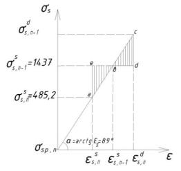
Using the diagram presented in Fig. 1, c and calculated value of internal forces in rebars, it is possible to determine additional dynamic stresses in rebars of an element in flexure at the moment of crack formation.

13

Scientific Herald of the Voronezh State University of Architecture and Civil Engineering. Construction and Architecture

An example of the calculation of additional dynamic stresses in rebars of a reinforced

concrete element under bending. The proposed method for the calculation of additional dynamic stresses in rebars has been tested in the calculation of a prestressed reinforced concrete beam with a rectangular cross section [19].

The test sample represented a single-span prestressed reinforced concrete beam of 1200 mm length with cross-sectional dimensions 60×140 mm and with concrete grade of B30. The beam was reinforced with prestressed rebars of A500 grade, diameter of 6 mm with prestressing force

P = 11,69 kN. Rebars in a compression area are of A400 grade with the diameter of 6 m; transverse rebars are of B500 grade with the diameter of 6 mm placed 100 mm away from each other. All the material grade are taken as adopted in the Russian regulations.

The calculation is performed with the following inputs: the height of cross-section is

h = 140 mm; the width of cross-section is b = 60 mm; a concrete cover in a tension area

aS = 15 mm; the diameter of prestressed rebars is d = 6 mm; the area of rebars is AS = 0,283 cm2; Rs,ser = 540 МPа, RS = 435 МPа, ES = 20 * 104 МPа; concrete grade В30, Rb = 17 МPа, Rb,ser = 22 МPа, Rbt = 1,2 МPа, Rbt,ser = 1,8 МPа, Eb = 32,5 * 103 МPа.

The parameters needed for the calculation of a tension force in concrete adjacent to a crack are the effective height of a cross section: h0 = 125 mm; parameters characterizing the size of a compression area of concrete adjacent to a crack: tb = 12 mm; t* = 9 mm; the relative height of a compressed area of concrete with cracks ξ = 0,217; k = 0,952; parameter В = 135,7;

σS = 267,54 MPa; σbt,c =42,7 MPa; shear force T = 15,4 kN; coefficient B4 = 0,9999. Checking the condition (13): 0<0,999<5,1. The condition is satisfied.

The design bending moment corresponding to crack formation is Mcrc = 2138 kN·m. Prestressing force P1 = 11,69 kN.

n-times statically indeterminate system.

A compression force under concrete and tensile stresses in rebars can be deduced from equa-

The values of stresses can be determined on the basis of the energy method using the diagram

14

Fig. 3. Diagram σS-εS for determination of dynamic stresses in rebars of (n-1)-times statically indeterminate system

Conclusions

1.The developed analytical relations can be used for the assessment of additional dynamic stresses in rebars of prestressed reinforced concrete flexural elements;

2.The proposed relations can be used for the assessment of structural survivability parameters for structures with prestressed flexural elements in states beyond the design basis.

References

1.SP 63.13330.2012 Concrete and reinforced concrete structures. General provisions. Updated version of SNiP 52-01-2003 – p. 66, 2012.

2.Eurocode 2 BS EN 1992-1-1:2004 Design of concrete structures. General rules and rules for buildings, p 70.

3.Geniev G. A. On assessment of dynamic effects in bar systems of fragile materials. Concrete and reinforced concrete, 1992, no. 9, pp. 25––27.

4.Geniev G. A. O dinamicheskikh effektakh v sterzhnevykh sistemakh iz fizicheski nelineynykh khrupkikh materialov [About dynamic effects in rod systems made of physically nonlinear brittle materials].

Promyshlennoe i grazhdanskoe stroitel'stvo, 1999, no. 9, pp. 23––24.

5.Travush V. I. Bezopasnost' i ustoychivost' v prioritetnykh napravleniyakh razvitiya Rossii [Safety and sustainability in priority directions of development of Russia]. Akademiya, 2006, no. 2.

6.Bondarenko V. M., Kolchunov V. I. Ekspozitsiya zhivuchesti zhelezobetona [Exposure the durability of reinforced concrete]. Izvestiya vuzov. Stroitel'stvo, 2007, no. 5, pp. 4––8.

7.Bondarenko V. M., Kolchunov V. I., Klyueva N. V. Eshche raz o konstruktivnoy bezopasnosti i zhivuchesti zdaniya [Once again on structural safety and resilience of buildings]. RAASN. Yubileynyy vypusk k 15-letiyu RAASN. Vestnik otdeleniya stroitel'nykh nauk, 2007, no. 11, pp. 81––86.

8.Karpenko N. I., Kolchunov V. I. O kontseptual'no-metodologicheskikh podkhodakh k obespecheniyu konstruktivnoy bezopasnosti [Conceptual-methodological approaches to ensure the structural safety].

Stroitel'naya mekhanika i raschet sooruzheniy, 2007, no. 1, pp. 4––8.

15

Scientific Herald of the Voronezh State University of Architecture and Civil Engineering. Construction and Architecture

9.Kolchunov V. I., Klueva N. V., Androsova N. B., Bukhtiyarova A. S. Structural survivability at actions beyond design basisю Moscow, АSV Publ., 2014. 208 p.

10.Klueva N. V., Emelyanov S. A., Kolchunov V. I. Criterion of crack resistance of corrosion damaged concrete in plane stress state. Procedia Engineering, 2015, no. 117(1), pp. 179––185.

11.Bondarenko V. M, Kolchunov Vl. I. Calculation models of reinforced concrete. Мoscow, ASV Publ., 2004. p. 472.

12.Salnikov A., Kolchunov V., Yakovenko I. The computational model of spatial formation of cracks in reinforced concrete constructions in torsion with bending. Applied mechanics and materials, 2015, vol. 725––726, pp. 784––789.

13.Golishev A. B., Bachinskii V. L., Polishchuk V. P. Reinforced concrete structures. Reinforced concrete structural mechanics. Kiev, Logos Publ., 2003. 414 p.

14.Veryuzhsky Yu. V., Golishev A.B., Kolchunov Vl.I. Handbook of structural mechanics. In two volumes. vol. I: Study guide. Moscow, ASV Publ., 2014. 640 p.

15.Veryuzhsky Yu. V., Klueva N.V. Methods of reinforced concrete mechanics. Kiev, НАУ Publ., 2005. 653 p.

16.Klueva N. V., Kolchunov V. I., Yakovenko I. A. Problems of development of fracture mechanics hypotheses with regard to reinforced concrete structures. News of KSUAE, 2014, vol. 3, pp. 41––45.

17.Klueva N. V., Kolchunov Vl. I., Yakovenko I. A., Gornostaev I. S. Deformations of reinforced concrete layered structures with shear cracks. Structural Mechanics and Analysis of Structures, 2014, vol. 5, pp. 60––66.

18.Kolchunov V., Osovskih E., Afonin P. On strength reserve assessment for prismatic folded plate roof structures. Applied Mechanics and Materials, 2015, vol. 725––726, pp. 922––927.

19.Rypakov D. A. Calculation of additional dynamic stresses in reinforced concrete elements in bending with torsion at the moment of crack formation. Housing construction, 2015, no. 3, pp. 19––22.

20.Seredin P., Goloshchapov D., Kashkarov V., Ippolitov Y., Bambery K. The investigations of changes in mineral-organic and carbon-phosphate ratios in the mixed saliva by synchrotron infrared spectroscopy. Results in Physics, 2015, vol. 6, pp. 315––321. doi: 10.1016/j.rinp.2016.06.005.

16

HEAT AND GAS SUPPLY, VENTILATION, AIR CONDITIONING,

GAS SUPPLY AND ILLUMINATION

UDC 644.1

S. N. Kuznetsov1

ORGANIZATION OF EFFECTIVE AIR EXCHANGE IN INDUSTRIAL PREMISES

Voronezh State Technical University

Russia, Voronezh, tel.: +7 (4732) 71-53-21, e-mail: kuznetvrn@mail.ru

1 D. Sc. in Engineering, Prof. of the Dept. of Heat and Gas Supply and Oil and Gas Business

Introduction. The development of energy-efficient schemes of organization of air in industrial premises requires consideration of the nature of air movement is displaced, which depends on the type of air distribution.

Results. A mathematical model of the spread of air in the room using the continuity equation, Reynolds averaged system stationary Navier-Stokes equations and k- turbulence model is set forth.

The most effective one is the ventilation circuit with fresh air supply jets plane vertically down the center of the room, and at an angle 20 to the vertical on the sides of the room. At the same time fresh air enters the work area, and only then removed local suction. Rising flows are above the bath and take out harmful substances from the work area to the upper area of the premises.

Conclusions. The proposed approach makes it possible to calculate and choose a system of air currents in the premises, the most effective uses fresh air and enhance ventilation efficiency at no additional cost.

Keywords: ventilation, air distribution, mathematical model

Introduction

Developing energy-efficient schemes of organizing air exchange in industrial premises requires considering the character of the motion of the air in a premise which depends on a selected type of air distribution. The financial and labour costs of studies into air exchange in natural conditions are very high. Therefore in order to address this, the method of mathematical modelling is currently used [3, 7, 9, 12, 15, 16, 20].

Mathematical model. A mathematical model of ventilation of air distribution is based on the discontinuity equation, the system of the Reynolds averaged Navier-Stokes equations and equations of k- turbulence models [1, 2, 6, 8, 17, 18, 19]. Let us look at the major equations of the model.

© Kuznetsov S. N., 2016

17

Scientific Herald of the Voronezh State University of Architecture and Civil Engineering. Construction and Architecture

The discontinuity equaiton is as follows:

where is the density of the air, kg/m3; xi - i–th spatial coordinates, m; ui are speed components of the air flow, m/sec.

The Navier-Stokes equation is as follows:

where p is the pressure, Pа; is a dynamic viscosity, kg/m seс; t is a turbulent dynamic viscocity kg/m seс; g is the free fall acceleration, m/seс2; k is the kinetic energy of turbulence, m2/seс2; j = 1, 2, 3; ij is the Kronecker symbol.

The transfer of the kinetic energy of turbulence in the standard k-ε model is given by the equations:

where is the speed of dissipation of turbulence energy, m2/seс3; С are the constants of the turbulence model; t is a turbulent dynamic viscosity, kg/m seс; k and are turbulent Prandtl numbers for k and . The turbulence speed is

18

The turbulent dynamic viscosity is given by the equation:

For the constants of the k-ε turbulence model, the following are accepted [4, 5, 10, 11, 13, 14]:

C1 1,44;C3 1,40;C2 1,9; k 1,0; 1,2.

The boundary conditions at the solid boundaries are determined by the conditions of adherence, sliding of the air specified for a speed vector at the solid boundaries. The boundary conditions at the free boundary are determined by the pressure, speed wind along the boundary normal or at the normal angle, conditions of leaking of the air with a zero pressure gradient.

The MatLab package in combination with the programming language C++ were used as environments of developing the software implementing the mathematical models of ventilation. Using the developed program the distribution of two-dimensional stationary air flows in a transverse section of the plant with local suctions in order to identify the impact of a method of supplying inlet air on the circulation of air flows was studied.

Calculation using the mathematical model. The object of the study was a two-dimensional section of the plant with industrial baths with the external sizes: the width of 1100 mm and the height of 1000 mm. The baths were placed in four rows in the transverse section of the plant and fitted with a two-sided lateral exhaust. The premises of the plant has the width of 36,0 m and the height of 12,0 m. The design order of air exchange was 16 h-1. The temperature of enveloping structures of the premises and inlet air was accepted to be 18 С. The air was supplied into the passages between the baths by air distributors.

19

Scientific Herald of the Voronezh State University of Architecture and Civil Engineering. Construction and Architecture

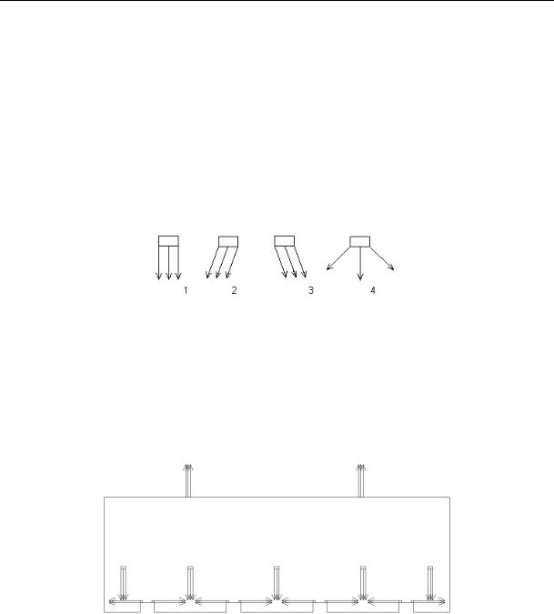
Three options of inlet air supply at the height of 0,6h from the floor were the following:

––flat flows with the vertical-bottom air;

––incomplete fan flows using perforated air supplier with a round section, the angle of the flow aperture of 45 and bottom air supply;

––flat flows with the vertical-bottom air supply in the centre of the premises and at the angle of 20 to the vertical along the sides of the premise.

The schemes of modelling the inlet air supply are identified in Fig. 1.

Fig. 1. Schemes of modelling the inlet air supply: 1 is a flat flow; 2, 3 is a flat flow with the air supply at the angle of 20 to the vertical; 4 is incomplete fan flow

Polluted air was removed from the premises of the plant using lateral exhausts from the baths with 90% of the total amount of the inlet air and 10% from the upper area through the duct in the plant, see Fig. 2.

Fig. 2. Schemes of the premise. The arrows show the supply and removal of the air

The results of the calculations are in Fig. 3––6.

The analysis of the results from Fig. 3––6 allows us to draw a few conclusions. An air flow from the air distributors moves down, interacts with the circulation areas and enveloping structures, reflects off the floor, turns and giving some of the air to the local suctions goes up. In all of the options along both sides from bottom inlet flows there are circulation areas. The size of the circulation areas along the horizontal is roughly half of the distance between the air distributors and along the vertical the height of the setup of the air distributors.

20