Учебное пособие 1862

or transient analysis time-domain node voltages and digital states. If these are the result of an operating point only run, the display shows the DC operating point values.

• Current: This option displays the last AC, DC, or transient analysis time-domain currents.

• Power: This option displays the last AC, DC, or transient analysis time-domain power.

• Condition: This option displays the last AC, DC, or transient analysis time-domain conditions. Conditions define the operating state for devices such as ON, OFF, LIN, SAT, and HOT for BJTs.

• Pin Connections: This option displays a dot at the location of each pin. This helps you see and check the connection points between parts.

• Grid: This option displays the schematic grid.

• Cross-hair Cursor: This option adds a cross-hair cursor.

• Border: This option adds a border to the schematic.

• Title: This option adds a title block to the schematic.

• Show All Paths: This command displays a list of all possible digital paths together with their delays. Selected paths are highlighted on the schematic. This is an immediate command as opposed to the Point to End Paths and Point to Point Paths modes, which require mouse clicks to specify path endpoints before a path list appears.

• Preferences: (CTRL + SHIFT +P) This accesses the Preferences dialog box, where many user preferences are chosen. These include:

59

•Common Options: This accesses a list of operational choices:

•File Warning: This provides a warning when closing an edited file whose changes have not yet been saved.

•Sound: This controls the use of sound for warnings and to indicate the end of a simulation run.

•Quit Warning: This provides a warning when quitting.

•Lock Tool Bar: This option disables movement and locks the tool bar into its current position.

•Print Background: If enabled, this option adds the userselected background color to the printouts. It is usually disabled, since most background colors do not print well.

•Select Mode: This option causes the schematic mode to revert to Select mode after any other mode is completed. For example, to place a component you must be in the Component mode. After placing the component, the mode normally stays in Component mode. If this option is selected, the schematic mode reverts to Select immediately after a component is placed. The same thing would happen when drawing wires, placing text, querying a component, or any other mode-based action.

•Time Stamp: This option adds a time stamp to all numeric output files and plots.

•Date Stamp: This option adds a date stamp to all numeric output files and plots.

•Package Library Load: If this box is checked, the Package Library is loaded when MC6 is first run. Otherwise it is loaded only when the Package editor is accessed. This option avoids the library load time for users who aren't using it.

•File List Size: This value sets the number of file names to include in the Recent Files section of the File menu.

•Warning Time: This sets the duration of warning messages.

•Floating Nodes Check: This provides a warning for floating nodes (those for which only one component pin is attached).

•DC Path to Ground Check: This checks for the presence of a DC path to ground. It should normally be on.

60

•Add DC Path to Ground: This option automatically adds a 1/GMIN resistor to any path where there is no path to ground.

•Plot on Top: If enabled, this option places the analysis plot on top of the schematic if they are overlaid. If unchecked, the schematic floats above the plot.

•Inertial Cancellation: If enabled, this option causes the logic simulator to employ inertial cancellation, which cancels logic pulses whose duration is shorter than the device delay. If this option is disabled, the simulator does not cancel short pulses.

•Analysis Progress bar: If enabled, this option displays a progress bar during a simulation run in the Status Bar area, if the Status Bar feature is enabled on the Options menu.

•Gmin Stepping: If enabled, this option tries gmin stepping after both normal methods and source stepping have failed to achieve DC convergence.

Text Increment: This controls whether non-command grid text is incremented during a paste, step, drag copy, or mirror operation. Incrementing means that the ending numerals in the text are increased by one. If no numerals are present, a T is added to the text.

•Node Snap: This flag compels components, wires, and text to originate on a node if a node's pin connection dot is within one grid of the object being placed or moved.

•Auto Show Model: This mode causes model statements added to the schematic text area by the Model command to automatically split the circuit window and show the newly added model statement. The advantage is that the user is shown where the model statement has been placed. The disadvantage is that the user may prefer a full-size screen.

•Component Cursor: If enabled, this option replaces the mouse arrow with the shape of the currently selected component whenever Component mode is active. This has the advantage of showing the currently selected component and its size.

61

•Rubberbanding: If enabled, this option causes drag operations to extend the circuit wires to maintain node connections. If disabled, drag operations sever selected wires at their endpoints and drag them without changing their shape or length.

•Show Slider: If enabled, this option places a slider control on the schematic adjacent to batteries and resistors during Dynamic DC Analysis. This lets the user change the battery or resistor values by dragging the slider with the mouse. With or without the slider, the values can be changed by regular amounts with each press of an UP ARROW or DOWN ARROW cursor key.

•Nodes Recalculation Threshold: If the Show Nodes option is enabled, nodes are recalculated and displayed whenever any schematic editing is done. For large schematics this can become time consuming. This value sets an upper limit for node count beyond which automatic node recalculation will be ignored, even if the Show Nodes option is enabled.

•Color Palettes: This option lets you define your own palettes. Click on any of the color squares to invoke a color editor that lets you customize the hue, saturation, and luminance of the selected palette color.

•Format: This option controls the numeric format to be used when displaying analysis plot tag values, schematic node voltages, currents, powers, DC operating point values in the numeric output text page, and schematic path delays. There are two basic formats:

<number> for standard notation <number>E for scientific notation

<number> represents the number of digits to the right of the decimal point. The <number>E format uses scientific notation to represent the number and <number> uses conventional notation.

•Status Bar Text: This lets you change the Status bar text attributes.

•Main Tool Bar: This panel lets you select the buttons that will appear in the six tool bars of the Main tool bar area. These tool

62

bars are called File, Edit, Component, Windows, Options, and Analysis. It also lets you show or hide individual tool bars.

•Component Palettes: This lets you name the nine component palettes and control their display in the Main tool bar. You can also toggle their display on and off during schematic use with CTRL + palette number.

•Default Properties For New Circuits: This dialog box controls the properties of new circuits. It includes:

•Schematics: This provides two types of features for schematics

•Color/Font: This provides control of text font and color for various schematic features such as component color, attribute color and font, and background color.

•Title Block: This panel lets you specify the existence and content of the title block.

•Tool Bar: This panel lets you select the buttons that will appear in the local tool bar area below the Main tool bar.

•SPICE Files: This provides two types of features for SPICE text files.

•Color/Font: This provides control of text font and color for

SPICE text files.

•Tool Bar: This panel lets you select the buttons that will appear in the local tool bar area below the Main tool bar.

Analysis Plots: This provides control for several analysis plot features:

•Colors, Fonts, and Lines: This provides control of text font and color for various plot features such as general scale and title text, window and graph background colors, and individual waveform color, thickness, and pattern.

•Scales and Formats: This panel lets you specify the numeric format for the Numeric Output window values, plot scales, and Cursor mode table values. It allows selection of Same Y Scales for separate plot groups and lets you select among three methods for measuring slope:

63

normal, dB/octave, and dB/decade. The latter two being more appropriate to certain AC measurements.

•Tool Bar: This panel lets you select the buttons that will appear in the local tool bar area below the Main tool bar.

•3D Plots: This provides control for several 3D plot features:

•Color: This provides color control of 3D plot features such as general scale and title text, window and graph background colors, axis colors, patch color, and surface line color.

•Font: This provides font control for all text in the 3D plot.

•Scales and Formats: This panel lets you select the numeric format for the X, Y, and Z axis scales and the numeric values in the cursor tables.

•Tool Bar: This panel lets you select the buttons that will appear in the local tool bar area below the Main tool bar.

•Monte Carlo Histograms: This provides control for Monte Carlo histogram plot features:

•Color: This provides color control of histogram features such as general scale and title text, window and graph background colors, and bar colors.

•Font: This provides font control for all text in the histogram.

•Tool Bar: This panel lets you select the buttons that will appear in the local tool bar area below the Main tool bar.

•Performance Plots: This panel controls performance plot features:

•Colors, Fonts, and Lines: This provides control of text font and color for various plot features such as general scale and title text, window and graph background colors, and individual plot color, thickness, and pattern.

•Scales and Formats: This panel lets you select the numeric format for plot scales and values shown in the

Cursor tables. It also allows selection of same Y scales for separate plot groups.

64

• Tool Bar: This panel lets you select the buttons that will appear in the local tool bar area below the Main tool bar.

• Global Settings: (CTRL + SHIFT + G) This accesses the Global Settings dialog box where many simulation control choices are made. These settings are discussed in greater detail in the Global Settings section of the Circuit editor chapter of the Reference Manual.

•User Definitions: This option loads the file MCAP.INC. This file, located on the directory with MC6.EXE, stores global definitions for use in all circuits. The contents of the file are automatically included in all circuit files.

•Component Palettes: This option accesses the Component Palettes. These provide a quick and convenient alternative to the Component menu when choosing components for placement in the schematic. Membership in a palette is specified from the Component editor. The original disks provide several sample palettes containing common analog and digital components. The palettes can be tailored to suit personal preferences. Palette display can be toggled on and off by pressing CTRL + palette number. For example, CTRL + 1 toggles the display of palette 1.

The Analysis menu

The Analysis menu is used to select the type of analysis to run on the circuit in the active window. It provides these options:

• Transient: (ALT + 1) This option selects transient analysis. This lets you plot time-domain waveforms similar to what you'd see on an oscilloscope. AC: (ALT + 2) This option selects AC analysis. This lets you plot frequency-domain curves similar to what you'd see on a spectrum analyzer. DC: (ALT + 3) This option selects DC sweep analysis. This lets you plot DC transfer curves similar to what you'd see on a curve tracer.

65

• Dynamic DC: (ALT + 4) This option selects an analysis mode in which the program automatically responds to user edits by finding and displaying the DC solution to the current schematic. You can change resistor values and battery voltages with slider controls or with the cursor keys. You can also make any edit such as adding or removing components, editing parameter values, etc. MC6 responds by calculat-

enabled, and device conditions if is enabled.

•Transfer Function: (ALT + 5) This option selects an analysis mode in which the program calculates the small signal DC transfer function. This is a measure of the incremental change in a user-specified output expression, divided by a very small change in a user-specified input source value. The program also calculates the input and output DC resistances.

•Sensitivity: (ALT + 6) This option selects an analysis mode in which the program calculates the DC sensitivity of one or more output expressions to one or more input parameter values. The input parameters available for measurement include all parameters that are available for Stepping, which is practically all model parameters, all value parameters, and all symbolic arameters. Thus you can create a lot of data with this analysis. A suitably smaller set of parameters is specified in the default set, or you can select only one parameter at a time.

•Probe Transient: (CTRL + ALT + 1) This selects transient analysis Probe mode. In Probe mode the transient analysis is run and the results are stored on disk. When you probe or click part of the schematic, the waveform for the node you clicked on comes up. You can plot all of the variable types, from analog node voltages to digital states. You can even plot expressions involving circuit variables.

•Probe AC: (CTRL + ALT + 2) This option selects AC Probe mode.

•Probe DC: (CTRL + ALT + 3) This option selects DC Probe mode.

66

The Design menu

The Design menu accesses the filter design functions.

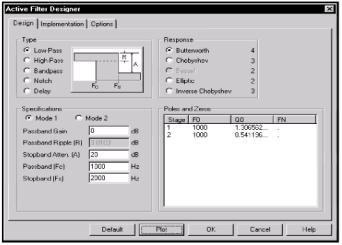
•Active Filters: This section accesses the Active Filter Designer. This part of the program designs an active filter from your filter. The filter type can be low pass, high pass, bandpass, notch, or delay. The filter response can be Butterworth, Chebyshev, Bessel, elliptic, or inverse-Chebyshev. The filter polynomials are calculated and implemented in one of several different circuit styles, ranging from classical Sallen-Key to Tow-Thomas. Optional plots of the idealized transfer function are available. Filters can be created as circuits or as macro components.

•Passive Filters: This section accesses the Passive Filter Designer. This part of the program designs a passive filter from capacitors and inductors from your filter specifications. The filter type can be low pass, high pass, bandpass, or notch. The filter response can be Butterworth or Chebyshev. The filter polynomials are calculated and implemented in either standard or dual circuit configuration. Optional plots of the idealized transfer function are available. Filters can be created as circuits or as macro components.

Figure 2-19 The Active Filter Designer

67

The Help system

The Help system provides information on the product in several ways:

•Contents: This section provides help organized by Menus and Topics.

•Search for Help On: The search feature lets you access information by selecting a topic from an alphabetized list.

•Product Support: This option provides technical support contact numbers.

•Email Spectrum: This lets you send an email to the Spectrum Software technical support group. Provision is made for your message and attachments like circuits or libraries. Your communications channel must be open before sending the email.

•About Micro-Cap: This option shows the software version number.

•Demos: These live demos show the sequence of actions involved in performing some of the MC6 functions. The demos include:

•General Demo: This provides a general overview of MC6. It includes each of the demos below and runs continuously until ESC is pressed.

•3D Plots Demo: This illustrates the use of 3D plots, which let you show how circuit waveforms or performance functions vary with two different parameters.

•Analog and Digital Demo: This shows how to mix analog and digital parts in a schematic and their analysis plots.

•Analysis Demo: This shows how to start and control an analysis.

•Animation Demo: This illustrates the use of the animation feature, in which animated circuit parts like switches, LEDs and seven-segment displays respond to circuit states by turning on and off.

68

•Dynamic DC Demo: This demonstrates the Dynamic DC feature, which automatically calculates the DC operating point of the circuit as it is changed by the user.

•Filter Demo: This illustrates the use of the integrated active and passive filter design function.

•Fourier Demo: This illustrates the use of the DSP functions to

do Fourier analysis on circuit waveforms.

•Monte Carlo Analysis Demo: This illustrates the use of Monte Carlo analysis, which analyzes circuit behavior statistically as circuit parameters are varied around specified distributions.

•Performance Plots Demo: This illustrates the use of performance plots, which let you plot important circuit characteristics, like bandwidth or rise time, versus model and other parameters.

•Probe Demo: This illustrates the use of the Probe feature, which lets you plot waveforms by clicking on schematic nodes or components.

•Schematic Demo: This shows how to create a schematic.

•Sensitivity Demo: This illustrates the Sensitivity analysis mode, which calculates the DC sensitivity of the circuit to one or more parameters.

•Stepping Demo: This illustrates the Stepping feature, which lets you systematically step or change model and other parameters to see their effect on circuit behavior.

•Subcircuits Demo: This demo shows how to create and use new subcircuits, including how to add them to the Component library.

•Transfer Function Demo: This illustrates the Transfer Function analysis mode, which calculates the DC transfer function.

The Component editor

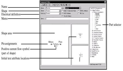
The list of components available for use in a schematic is called the Component library. It is managed by the Component editor which looks like this:

69

Figure 2-20 The Component editor

To create a component you specify the Name, Shape, Definition, Initial Text Attribute Locations, and Pin Assignments. Subcircuits, macros, logic expressions, pin delays, and constraints require named pins.

Name is the proper name of the component. It appears in the Component menu when you select a component to add to a circuit.

Shape is the name of the shape that is drawn when the part is placed in a circuit. This name is chosen from a list of named shapes created and maintained by the Shape editor. Clicking in the field displays the list.

Definition specifies the general mathematical model to be used. Numeric parameter values to be used in the model are specified in a model statement contained in or referenced by the circuit. Clicking in the field displays a list of definitions.

Memo is used for descriptive information about the part or its function. It has no effect on electrical behavior.

Initial Text Attribute Locations are specified by dragging a generic text block to the desired location relative to the shape for the two orientations. This specifies the initial text location, when the part is first placed in a schematic.

Pin assignments equate visible pin locations with the electrically defined pin names. When you add a part like an NPN transistor, pin

70

names automatically appear and need only be dragged to their proper locations on the shape. Macros, subcircuits, logic expressions, pin delays, and constraints require the user to place a pin and name it. Placing is done by clicking in the Shape area, typing a pin name in the Pin dialog box, specifying whether it's an analog or digital pin, then dragging the pin to a suitable location on the shape.

Editing an existing pin name involves double-clicking on the pin dot or pin name to invoke the Pin Name dialog box. Pins and their names may be independently located on the shape by dragging the pin dot or the pin name. Some digital parts have a variable number of pins and require an additional Pin field to specify the number of input, output, and enable pins. For example, a nor gate may have an unlimited number of inputs. An Input field then specifies the number of inputs.

The Model = Component Name option, if selected, automatically assigns the component name to the model name when the component is added to a schematic. This bypasses the Attribute dialog box, simplifying the process of adding components. This option is enabled on all Analog Library and Digital Library parts and is disabled on all Analog Primitive and Digital Primitive parts.

The PART, VALUE, and MODEL attribute options, if selected, set the display flag for these attributes. Some parts have no MODEL or VALUE attribute. If you place a part with this flag enabled, the attribute text will be initially displayed. You can turn it off through the Attribute dialog box by disabling the display flag. This option only affects the initial setting of the display flag.

The PIN Text option, if selected, sets the initial display flag for showing pin names. This flag can be individually changed on the part when it is placed in a schematic. This flag is normally enabled for complex LSI parts, and disabled for simpler components, such as diodes and transistors, since their shapes adequately identify the pin names. For example, it's easy to identify the base lead of an NPN, but not so easy to identify the pin names on a digital ALU or complex linear part.

The Palette field lets you assign the displayed part to one of the nine custom user palettes. These pop-up palettes are designed to make

71

component selection easier for frequently used parts. The palettes are invoked with CTRL + palette number.

The New File button creates a new component library file. The Open File button opens an existing component library file.

The Merge button lets you merge an MC4 (*.MC4), an MC5 (*.MC5), or an MC6 component library file with the current MC6 component library file.

The Add Component button adds a new component to the group selected in the hierarchical list. To add a component, select a group or component from the list, click this button, then edit the name and other fields.

The Add Group button adds a new group at the end of the group currently selected in the hierarchical list. To add a group, select a group from the list, click this button, then edit the generic group name that appears.

The Copy button copies the current component description to the clipboard in preparation for a subsequent paste to the library.

The Paste button copies a component description from the clipboard to the library. The new component is a copy of the clipboard version except for the name, which is generic. The purpose of this command is to simplify the process of entering many components that are identical except for one or more attributes.

The Delete button deletes the shape from the currently open library.

The Zoom-In button makes the shape larger. The Zoom-Out button G^| makes the shape smaller.

The Clear Palettes button removes all component names from the user-defined component palettes.

The Help button provides information for the Component editor. 72

As originally supplied, the component library contains all of the components that you ordinarily need. Its principal use is to define new macro and subcircuit components. You might find it desirable to add your own common components, perhaps with unique or customized shapes.

Ответьте на вопросы:

1.Какие инструменты использует редактор Shape editor?

2.Какие функции включает в себя Model editor?

3.Что Вы узнали об используемых функциональных клавишах?

4.Скажите, что говорится в тексте о:

а) Назначении функции Undo

б) Type Selector

в) Part Selector

5.Найдите подтверждение в тексте о том, что Model

– отдельная программа Windows, которая создает аналоговые образцовые параметры.

6.Каким образом можно быстро переходить от одной рабочей панели к другой?

The Shape editor

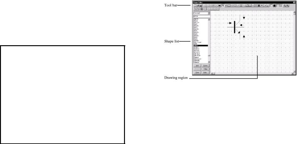
The Shape editor is used to create and maintain the shapes, or graphical images used to represent the component in a schematic. It looks like this:

73

Figure 2-21 The Shape editor

Shapes are created by selecting drawing tools from the Tool bar and clicking or dragging the mouse in the Drawing region to create a graphical object.

The Scale buttons in the Tool bar change the display size of the shape image shown in the Drawing region.

The Add button adds a new shape. The Delete button deletes the currently selected shape. The Object editor button invokes an editor that lets you edit the specific numerical values that determine a particular object's size or other features.

The Tool bar provides many specific tools and objects which are described in more detail in the Reference Manual.

The Model editor

Model libraries provided with MC6 come in two forms, text and binary. In text form they are contained in files with the extension LIB, and encode device models as .MODEL, .MACRO, and .SUBCKT statements. Text files can be viewed and edited with any text editor, including the MC6 text editor.

74

In binary form, model libraries are contained in files with the extension LBR, and are implemented as a list of model parameters for the parts. These binary files can be viewed and edited only with the Model editor. The Model editor is invoked when the File menu is used to open or create a binary library file.

The Model editor should not be confused with the MODEL program, which is accessed from the Windows menu. MODEL is a separate Windows program which produces optimized analog model parameters from commercial data sheets. MODEL can create model libraries in either the text or binary form.

Once binary libraries are created, the Model editor can view and edit them. The Model editor display looks like this:

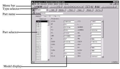
Figure 2-22 The Model editor

The various parts of the editor function as follows:

• Name: This field is where the part name is entered. If the part has been imported from the MODEL program, this field is a copy of the Tl text field.

75

•Memo: This is a simple text field that may be used for any descriptive purpose. If the part has been imported from the MODEL program, this field is a copy of the T3 text field.

•Type selector: This is used to select which device type to display. Each library may contain a mixture of different device types. Selecting NPN for example, displays all of the NPN bipolar transistors in the file.

•Part selector: This selects a part by name for display and possible editing. It provides a window to review the specific model values for the displayed part. As in other windows, the Maximize button may be used to enlarge the window to see more of the model values.

•Add: This adds a new part of the current device type to the current library.

•Delete: This deletes the displayed part.

•Pack: This removes all duplicated and untitled parts and reorders the parts alphanumerically.

•Copy: This command copies a part from the displayed library to a target library. If the target library already has a part with the same name, the name of the newly created copy is set to "name_copy". The target library may be the current library.

•Merge: This command merges a library from disk with the displayed library. The merged library is displayed and but not saved to disk.

•Go To: This command lets you specify a parameter name, then scrolls the parameter list of the currently displayed part to show the parameter value. Note that the Find function is available to locate parts by name in the current library file or in one of the library files

on disk. Simply click on the Find button in the Tool bar.

Function keys

Several function key combinations are dedicated to the most common operations:

76

Fl is used to invoke the Help system. It accesses an information data base by contents and by alphabetical index.

F2 is used to start an analysis after selecting the type of analysis from the Analysis menu.

F3 quits the AC, DC, or transient analysis and returns to the Schematic editor. F3 also repeats the last search when in the Schematic editor.

F4 displays the analysis plot.

CTRL + F4 closes the active window. F5 displays the Numeric Output window.

F6 scales and plots the selected analysis plot group. CTRL + F6 cycles through the open windows.

F7 switches the analysis plot to Scale mode.

F8 switches the analysis plot to Cursor mode.

F9 displays the Analysis Limits dialog box for AC, DC, or transient analysis or their Probe equivalents.

CTRL + F9 clears the waveforms in Probe and invokes the Analysis Limits dialog box when in an analysis module.

F10 invokes a dialog box for the front window that lets you change the front window characteristics. The type of dialog box depends upon the type of front window.

Fl 1 invokes the Parameter Stepping dialog box. F12 invokes the State Variables editor.

The Undo function

Most schematic and text editing can be reversed by using the Undo function. Only the last operation may be undone. Undo is accom-

plished by clicking on the Undo button or by pressing CTRL + Z. The Undo function is shown under the Edit menu.

For instance, if you add a component, then undo the operation, the component will be removed. If you edit a component parameter, Undo will restore the prior parameter.

77

The Undo function for schematic editing is reversible. For instance, if you move a component, repeatedly using the Undo function will cause the component to move back and forth between the original and new positions.

Schematic edits may be undone even after running an analysis. You can delete a region of circuitry from a circuit, run an analysis, then return to the Schematic editor and use the Undo function to restore the circuit to its former condition.

There is a separate Undo function for text fields. It is activated by the same CTRL + Z keys. This function restores the initial text of a text field after editing. The initial text is the text in the field when the field is first displayed. It is not reversible. That is, the text may not be toggled between old and new by repeatedly pressing the undo keys.

Note that the Revert command on the File menu also functions like a large-scale undo command. It loads the existing version of the front window file from disk, discarding any changes to the front window that occurred since it was loaded.

78