3.1Theory of Thin-Walled Beams Based on 3D Equations of the Theory of Elasticity

(surface forces are absent). The characteristics of the unperturbed equilibrium state satisfy the following geometrically nonlinear equations and boundary conditions on the surface [1]:

where dik is the Kronecker’s symbol, mj are the components of the unit vector normal to the boundary surface, Latin indices take on the magnitudes 1, 2, 3, a Latin index after comma denotes the partial derivative with respect to the corresponding spatial coordinate x1; x2; x3; and the summation is understood over the repeated indices.

Let us perturb the body with some small deviations from the unperturbed equilibrium: ui; rij; Xi ¼ q€ui; where q is the material density, and an overdot

where vi is the displacement velocity.

The components of the perturbed state satisfy the following equations and

Substituting (3.3) in (3.4) and (3.5), carrying out the linearization of the

Suppose that the unperturbed state deviates a little from the initial undeformed state. In the majority of engineering problems the given assumption is found to be valid. In this case, the terms u0i;k can be neglected, and Eqs. 3.2, 3.6 and 3.7 at r0ij ¼ cij; where cij ði; j ¼ 1; 2; 3Þ are certain constant values (moreover, some of them could be vanished according to the conditions of the problem under consideration), take the following form:

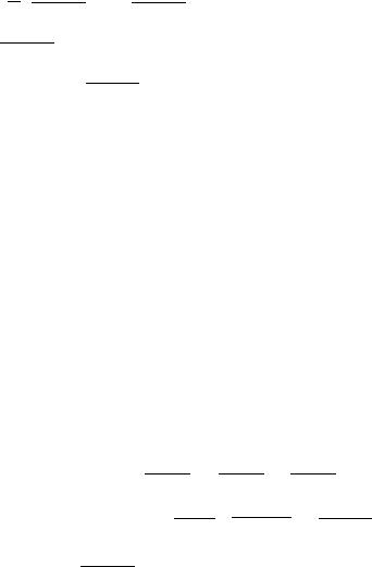
Fig. 3.1 Scheme of a spatially curved linear elastic beam of arbitrary open cross-section

where k and l are Lame constants.

Suppose that the wave surface of strong discontinuity exists in a spatially curved thin-walled beam of open section. Then let us differentiate (3.8), (3.11) and (3.9) k times with respect to time, write them on the both sides of the wave surface, and take their difference. As a result we obtain

Equation 3.13 lacks the discontinuities in the external forces, since they are continuous on the wave surface of strong discontinuity.

For the ease of further treatment, let us introduce two sets of coordinates:

k; s; n with the unit vectors kfkig; sfsig; and nfnig; and k; x, y with the unit vectors k; kfkig; and sfsig: The axes k; s; n are the natural axes for the curved axis

of the beam, in so doing the k-axis is the tangent to the beam’s axis, the s-axis is its binormal, the n-axis is its main normal, s is the arc length calculated from a certain point with the coordinate s0 along the beam axis (Fig. 3.1), while the x- and y-axes are the main central axes of the beam’s normal section. The angle uðsÞ is the angle between the x- and s-axes and the y- and n-axes.

where K ¼ du=ds; while ðsÞ and sðsÞ are the curvature and the torsion of the beam’s axis, respectively. Note that it is precisely these three values, K(s), ðsÞ and sðsÞ; that are of prime engineering interest in studying the spatially curved thin-walled beams of open profile. Moreover, as it will be shown in the further analysis, these values produce new features in the dynamic response of such beams as compared with straight thin-walled beams of open cross-section.

Considering the conditions of compatibility (see Sect. 6.1)

axial compression or tension stresses r0kk and their different combinations on the dynamic response of thin-walled rods of open profile is a very complicated problem which is of great importance in civil engineering and bridge construction.

However, reference to Eq. 3.22 shows that the value r0kk is multiplied by the k ? 1-order jump and by the s-derivative of the k-order, i.e. it has a strong impact both on the velocities of the surfaces of strong discontinuity and on the discontinuities, in contrast to the values r0kx and r0ky which are multiplied only by the k- and k - 1-order jumps, i.e. they exert weak effect only on the jumps. That is why, below in Sect. 3.1.2 , we shall neglect r0kx and r0ky with respect to the value r0kk:

3.1.2Dynamic Response of Axially Pre-Stressed Spatially Curved Thin-Walled Beams of Open Profile

Thus, assuming further that r0kx ¼ r0ky ¼ 0 and r0kk 6¼ 0; from (3.22) we have

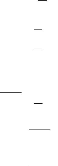
Fig. 3.2 Scheme of the cross section of a thin-walled beam with a generic open crosssection

Then the boundary surface will be free from the normal and tangential stresses. Now we expand the value ½vi;ðkÞ& entering into (3.21) and (3.23)–(3.26) in terms

of three mutually orthogonal vectors k; k, s. As a result we obtain

where xðkÞ ¼ ½vi;ðkÞ&ki; hðkÞ ¼ ½vi;ðkÞ&ki; and gðkÞ ¼ ½vi;ðkÞ&si:

Suppose that for a thin-walled beam of open section the following velocity fields (involving seven independent functions at each fixed k) are fulfilled [3]:

where s1 is the arc length measured along the cross-section profile from the point M0; which corresponds to the arc length of s01; to the point M½xðs1Þ; yðs1Þ&; which corresponds to the arc length of s1 (Fig. 3.2).

Gol’denveizer [3] proposed that the angles of in-plane rotation do not coincide with the first derivatives of the lateral displacement components and, analogously, warping does not coincide with the first derivative of the torsional rotation. Thus Gol’denveizer [3] pioneered in combining Timoshenko’s beam theory [4] and Vlasov thin-walled beam theory [5] and suggested to characterize the displacements of the thin-walled beam’s cross-section by seven generalized displacements.

In order to refine the structure of formula (3.28) in the case of a spatially curved thin-walled beam, let us differentiate (3.27), which involves only the terms x0ðkÞ; h0ðkÞ; and g0ðkÞ; with respect to s with due account for (3.15)–(3.17). As a result we obtain

Moreover, we shall use the relationship for the discontinuity in the k-order derivative with respect to time t of the angular velocity

Differentiating (3.32) with respect to s and considering (3.15)–(3.17) yields

If we suppose that transverse shear strains are absent, then we are led to the following relationships, which are in compliance with the Vlasov theory:

If we now substitute (3.34)–(3.36) in (3.28), then we obtain a formula for defining the k-order time-derivative in the discontinuity in the velocity of translation along the k-axis without account for transverse shear deformations.

26 3 Transient Dynamics of Pre-Stressed Spatially Curved Thin-Walled Beams

Following Gol’denveizer [3], in order to take the transverse shear deformations

Formulas (3.29) and (3.30) remain unchanged.

If we put K ¼ ¼ s ¼ 0 in (3.40), then we are led to the case of a straight thin-

by their magnitudes defined by formulas (3.37)–(3.39).

At k ¼ 0; the values entering in (3.29), (3.30) and (3.40) have the following physical meaning: x0ð0ÞðsÞ; h0ð0ÞðsÞ and g0ð0ÞðsÞ are the discontinuities in the velocities of translatory motion of the section as a rigid body together with the point C (the center of gravity of the cross-section) along the k-, x- and y-axes, respectively, x1ð0xÞðsÞ; x1ð0yÞðsÞ and x1ð0kÞðsÞ are the discontinuities in the angular velocities of the cross-section’s rotation as a rigid whole around the x-, y- and k-axes, respectively, wð0ÞðsÞ is the discontinuity in the velocity of warping of the cross section, xAðs1Þ is twice the area of the sector AM0M; the point A is the center of bending (Fig. 3.2) with the coordinates [5]

Moreover, the choice of the point A with the coordinates defined by formulas (3.41) results in the fulfillment of the following relationships:

Note that the sectorial area, generally speaking, depends on two coordinates, namely: the initial point s01 and the terminal point s11; i.e. xAðs01; s11Þ: Let us choose

F

will be valid. Then, as it is shown in [5], taking the point with the coordinate s11 as

the origin of the arc length measuring, we obtain

Z

Let us name this point as the null sectorial point [5]. Since there may exist several such points, the null sectorial point nearest to the point A can be named as the main null sectorial point, and we shall take it as the initial point of reading.

Thus, using the above mentioned choice of the coordinates and the initial points of measuring, the functions 1, xðs1Þ; yðs1Þ; and xAðs11; s1Þ; as formulas (3.42)– (3.45) show, occur to be orthogonal.

If we substitute (3.21) in (3.24) and (3.25) and consider (3.27), then we are led