Авдеев Е.Ф., Смирнова В.О. Конспект лекций по курсу Механика жидкости и газа eng

Fig. 6.1

It is necessary to determine these parameters in an arbitrary section of the channel A (x). The gas is considered ideal (without friction) and the parameters over the cross section are homogeneous. To solve these problems, 4 groups of isentropic formulas obtained below are used..

6.3.2. The concept of the speed of sound and the number M.

The speed of sound in a medium is the speed of propagation of waves of weak intensity, with a very small change in pressure and temperature. General expression for the speed of sound a in any environment:

Despite the fact that expression (6.8) is of a general nature, it is clear that the speed of sound will be the value in the medium where the density changes little with pressure.

So in pure water a = 1450 m⁄s, in saturated steam the average value is a = 400 m⁄s, in air a = 340 m⁄s, etc.

Newton's initial assumption about the isentropic propagation of sound waves led to erroneous results, which Laplace succeeded in correcting the adiabatic propagation of sound waves.

well matched with experience.

From the expression (6.9) it follows that the concept of the speed of sound at a point is

strict.

For the practice of operating NPPs, the concept of sound velocity in two-phase media will be of fundamental importance, which is qualitatively depicted in the graph of Fig. 6.2. The abscissa shows the volumetric vapor (or gas) content .

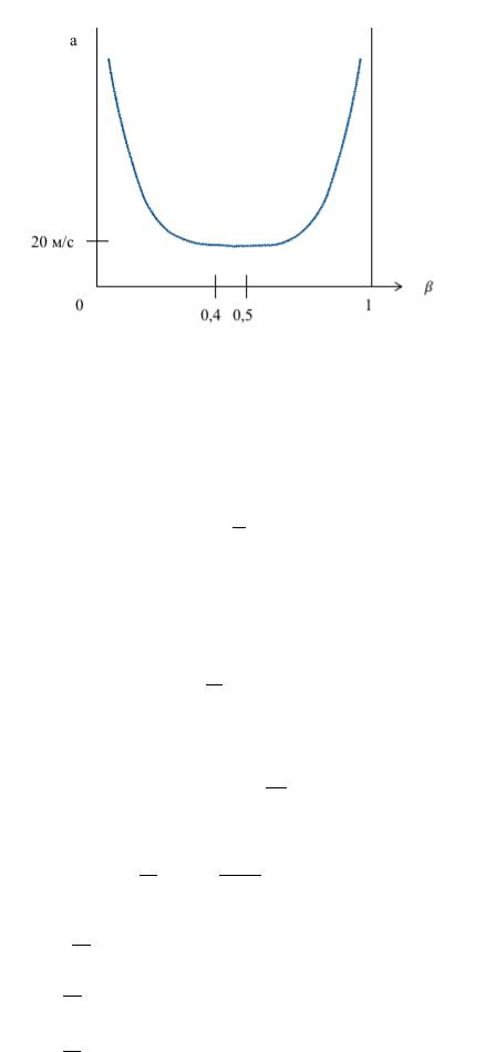
Fig. 6.2

t is seen that at β = 0.4 ÷ 0.5, the speed of sound can become a = 20 m⁄s. Without knowledge of these features of acoustics, it is impossible to explain many processes, especially emergency ones.

The number M, as the ratio of the velocity of the medium to the local speed of sound, in many manuals is referred to as the Mach number, named for the Austrian physicist. However, much earlier than Mach, it was introduced by the Russian ballist Mayevsky, whose name this number should be called, or simply the number M.

In the theory of similarity and physical modeling of the flow of compressible media, the number M is one of the criteria of similarity.

6.3.3 Isentropic formulas

From the thermal formula of the Bernoulli integral follows:

(6.10)

Determining the constant in (6.10) from the condition at the stagnation point, we obtain the relation between the enthalpy of inhibition and the static enthalpy:

a look:

( ) therefore, the relationship of the speed of sound will be equal:

This is the first group of formulas, connecting the parameters of inhibition and static, through the number M.

Simple reasoning we get three more groups of formulas,

-binding static parameters:

( )

⁄

( )

( )

⁄

( )

-static and critical parameters

Parameters are called critical in the place (or section) where the velocity of the medium is equal to the local speed of sound (M = 1). Normally, the critical speeds of a medium are .

-braking and critical parameters

( )

⁄

( )

( )

⁄

( )

Depending on the particular task, use one or another group of the above formulas.

From group (IV) it follows a very difficult to understand fact that there are many sound speeds in a given stream (different temperatures), and the critical speed is one. Since the enthalpy of braking (and hence the temperature of braking) remains the same, the critical temperature also remains the same. Therefore, the critical speed corresponding to it is the same.

.

6.4. Common problem solutions

The main condition will be to save mass flow in section A1, where the parameters are known, and in longitudinal section А(х):

where only the number M is unknown. It is found and put in the formula of group (II) to determine the static parameters in an arbitrary section A (x).

If the A1 section is critical (M1 = 1), expression (6.11) will be simpler:

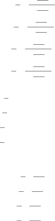
Graphic representations of the formula (6.12) are presented in Fig. 6.3.

Fig. 6.3

It is clear that in the area of subsonic speeds, in order to increase the speed, the crosssectional area of the channel needs to be reduced, and in the area of supersonic speeds, on the contrary, to increase.

While maintaining mass flow, an increase in speed and area can occur only due to a strong decrease in density. Let us proceed to the principle of operation of the refrigeration device, since in adiabatic processes the decrease in density is accompanied by a decrease in temperature.

6.4.1. Confusion nozzle outflow

This is a classic example of the formation of critical parameters in a narrow nozzle sec-

nozzle reaches the local sound velocity, since the change in p 'with the sound velocity is transferred to the outflow volume. But when in the exit section of the nozzle the velocity of the gas reaches the speed of sound, the perturbations p 'cannot penetrate into the outflow volume, since they are carried away by the gas flow. A phenomenon occurs that is present in the "locking" of

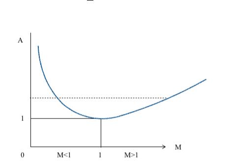
the nozzle exit section, when no matter how much p ^ 'decreases, the mass flow rate remains unchanged. The above is presented on the graph (Fig. 6.4), where the dimensionless flow is plotted along the ordinate axis.

that until the velocity in the output section reaches the speed of sound, the pressure in it is equal to the counterpressure, and the critical pressure is about half the pressure in the outflow volume

6.4.2. Outflow through a Laval nozzle

The nozzle is named after the Swedish engineer Laval, who proposed them for use in steam turbine guide vanes, since the transfer of the same mass flow rate to supersonic speeds in them increases the amount of motion before the turbine blades. Due to this, the force acting on

the tourbine's shoulder blade increases, because it is proportional to the difference in the amount of movement in front of and behind the shoulder blades.

Not always, reaching critical parameters in a narrow section of the nozzle, the speed in the expanding part of the nozzle becomes supersonic. It all depends on the back pressure at the nozzle exit. On the geometry of the nozzle, specifically in relation to the areas of the output sec-

̅̅̅̅. In the latter case, the nozzle will operate in the design, but supersonic mode. It is dangerous when:

̅̅̅̅̅

and in the expanding part of the nozzle a direct shock occurs, after which the speed will be subsonic. This direct compression shock will be discussed below.

ter the exit, an additional expansion and an increase in velocity occur. The last unplanned mode was successfully used by the author of these lectures for the gas-dynamic shut-off of the conduits

of neutron generators (see patents).

You need to know how to really perform to ̅̅̅

Пусть противодавление равно атмосферному давлению. Тогда, получив значения

̅̅̅

, It is necessary to replace through the braking pressure in the flow volume accord-

When creating a pressure in the volume of outflow p_0, the nozzle may not reach the supersonic mode, since the ideal gas formulas do not take into account the presence of a boundary layer near the nozzle walls, moreover, the flow in the diffuser part of the nozzle may acquire a twist. These discrepancies are selected by a minor change in the calculated p0. In other words, the student needs to know how to really bring the Laval nozzle to a supersonic mode.

It is also fundamentally important to know that the nozzle of a given geometry can have only a single supersonic mode with a specific number M at the output.

6.4.3. Shock waves and shock waves

It may seem strange that in the discipline readable by the future NPP operator, knowledge of shock waves is required, which (according to classical ideas) can occur only in supersonic flows. However, if we refer to the peculiarities of acoustics in two-phase media, the mixture velocity of 25 m⁄s can already be supersonic if the volume vapor (or gas) content β = 0.4 ÷ 0.5, which corresponds to very small values of the mass vapor (or gas). a) content.

Shock waves occur when conditions are created for the imposition of a large number of sound waves, which are known to carry a very small change in pressure and temperature. The imposition of sound waves will occur when each successive wave will have a speed greater than the previous one. Then a powerful compression wave arises with a finite change in pressure and

temperature at almost zero thickness (more precisely, at a thickness equal to the free range of molecules). It always moves with a supersonic speed θ and is called the ―shock wave‖. With its distribution, the processes in the gas are essentially non-stationary. Usually, motion is reversed in a frame of reference moving at a speed θ opposite to the direction of wave movement. In this frame of reference, the shock wave will be stopped, which is already called a shock wave. For

-of mass

-amount of movement

-of energy

where the index "1" indicates the parameters before the shock wave (must be known), and the index "2" - after the shock wave (requiring definition).

As is known, with the Poisson adiabat, the processes are isentropic, consequently, in the adiabatic system as a whole, the transition of gas through the shock wave will be accompanied by an increase in entropy. These adiabats are depicted graphically (Fig. 6.5).

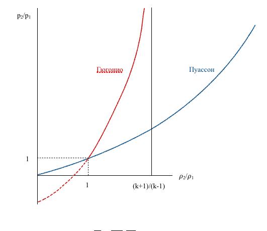
Fig 6.5

The adiabats have a common point (1; 1), but the Hugoniot shock adiabat has asymptotic restrictions on the density change: with

line (Figure X.5), the points of which lie below the Poisson adiabat, this means a decrease in entropy, which means the impossibility of a vacuum drop. However, if there will be an energy supply, discharge surges are possible, like other real processes with a decrease in entropy.

Congestion shocks that actually occur in two-phase flows, due to an increase in pressure, can lower the flow rate and even stop the flow of the coolant.

7. Features of hydraulic shock in a boiling coolant. Cavitation

Hydraulic shocks are a substantially non-stationary process in which waves of high pressure, normal recovered pressure, and low pressure alternate. They cause vibrations of the pipeline and its possible destruction.

7.1. Direct and indirect water hammer

The first who applied acoustics to explain the increased pressure during hydraulic shocks was N.E. Zhukovsky, who got the formula for maximizing pressure:

(7.1) where – sound velocity in the pipeline, taking into account the elastic properties of wa-

ter and wall material; – average speed.

Formula (7.1) is applicable in the case where the closing time of the valve less period of water hammer , where – the distance from the place of the final pressure perturbation

to the place of the reflection of the waves. This case is called the direct shock.

In the case of indirect water hammer ( ) maximum pressure increase can be estimated using the Michau formula:

(7.2)

The mechanism of indirect water hammer is so complex that today there is no general theoretical solution. The above applies to a hydraulic shock in a single-phase fluid and is described in the textbooks on hydraulics.

7.2. Boiling coolant

Elevated or reduced pressures in waves that move at the speed of sound persist during the period of water hammer T. Therefore, boiling up will occur in a liquid that is slightly underheated before saturation when a reduced pressure wave arrives, and the speed of the waves (sound velocity) decreases accordingly. After a period T, an increased pressure wave arrives at this place and the vapor bubbles ―collapse‖, which leads to an additional pressure increase, about 1.5 times the pressure increase in a single-phase medium. This is only an experimental fact, a theoretical solution has not yet been obtained.

7.3. Cavitation

Cavitation is sometimes called ―cold‖ boiling, it occurs when the pressure decreases or due to a local increase in speed (pipe rotation), when the pressure is equal to the saturation pressure at a given water temperature. If there is an area of high pressure nearby, vapor (or evolved gas) bubbles collapse, which leads to a combined effect on the wall material. Such repeated effects over a long time lead to a change in the crystal structure of the material, and the dyeing of the material begins. This is one mechanism, of course, the main one.

In addition, when a bubble appears on the wall, the molecular layer is destroyed, with an electric discharge slipping. This leads to the formation of corrosion-enhancing ozone.

The two mechanisms named are the cause cavitational destruction of the material..

8. Boundary layer

It is generally accepted that before the discovery in 1904 of L. Prandtl in the boundary layer, there was the empirical science of "Hydraulics", within which it was impossible to count the friction force on the wall. Later they began to classify the dynamic boundary layer (calculation of friction force), thermal boundary layer (calculation of heat fluxes) and diffusive layer (calculation of mass flow). In 2004, the world scientific community celebrated the 100th anniversary of the opening of the boundary layer, holding scientific forums in many countries.

8.1. Physical understanding of the boundary layer. Prandtl boundary layer equations

The boundary layer is a thin area near the wall, where the speeds, temperatures, and concentrations vary greatly (if the medium is multi-component).

The thickness of the dynamic boundary layer depends on viscosity . When where – is time.

Replacing the time on the path x divided by the speed U we get the relative value of the boundary layer:

Blausius obtained, for a laminar boundary layer, on a plate const = 5. Immediately, we note that the friction stress is determined by the thickness of the boundary layer δ.

Estimating the order of the terms in the Navier-Stokes equations for a thin region of the boundary layer of a two-dimensional flow (there will be two equations), using the continuity

and can be discarded. And in the equation of projection on the Y axis, all the terms of a high order of smallness, except . As a result, the equation remains for the boundary layer region:

(8.2)

These equations (practically one) will be the equations for the laminar boundary layer, for the latter is the law of conservation of mass.

The second equation means a very important property of the boundary layer: the pressure across the layer does not change. For this reason, the propagation pressure velocity at the boundary layer boundary will be the same as that on the wall.

with the calculated value.

Once Prandtl was given the boundary layer equations, Blausius found their exact solution for the laminar boundary layer on the length plate .

Friction stress:

√

Local coefficient of friction:

√

Full friction coefficient:

√

8.2. Integral relations of T. Karman

Blausius' solution path was unacceptable for engineers, so much later T. Karman proposed to write L. Prandtl’s equations in another form, which was called the integral relation:

– velocity change along the boundary layer boundary.