

Epidemiology for English speaking students / How to read a paper / Reading_statistics 2
.pdfHome |
Help |
Search |
Archive |
Feedback |
Table of Contents |
Author
Vol 
[Advanced]
Institution: Massey University Library Sign in to your Personal subscription
BMJ 1997;315:422-425 (16 August)
Education and debate
How to read a paper: Statistics for the nonstatistician. II: "Significant" relations and their pitfalls
Trisha Greenhalgh, senior lecturer a
a Unit for Evidence-Based Practice and Policy, Department of Primary Care and Population Sciences, University College London Medical School/Royal Free Hospital School of Medicine, Whittington Hospital, London N19 5NF p.greenhalgh@ucl.ac.uk
This article
Extract  Respond to this article
Alert me when this article is cited Alert me when responses are posted Alert me when a correction is posted View citation map
Services
Email this article to a friend Find similar articles in BMJ Find similar articles in PubMed Add article to my folders Download to citation manager Read articles citing this article
Google Scholar
Articles by Greenhalgh, T.
Articles citing this Article
Ads
Sta An
Th gui inf Sta
ww data
Wh Sig
Fre Tu Pra
sixs
Introduction
This article continues the checklist of questions that will help you to appraise the statistical validity of a paper. The first of this pair of articles was published last week.1
PubMed
PubMed Citation
Articles by Greenhalgh, T.
 Top
Top
 Introduction
 Correlation, regression, and...
 Probability and confidence
 The bottom line
 Summary
  References
Correlation, regression, and causation
Has correlation been distinguished from regression, and has the correlation |
Top |
|
Introduction |
||
coefficient (r value) been calculated and interpreted correctly? |
Correlation, regression, and... |
|
Probability and confidence |
||
|
||
|
The bottom line |
|
For many non-statisticians, the terms "correlation" and "regression" are |
Summary |
|
synonymous, and refer vaguely to a mental image of a scatter graph with dots |
References |
|
|
||
sprinkled messily along a diagonal line sprouting from the intercept of the axes. |
|
You would be right in assuming that if two things are not correlated, it will be meaningless to attempt a regression. But regression and correlation are both precise statistical terms which serve quite different functions.1
The r value (Pearson's product-moment correlation coefficient) is among the most overused statistical instrument. Strictly speaking, the r value is not valid unless the following criteria are fulfilled:
Summary points
An association between two variables is likely to be causal if it is strong, consistent, specific, plausible,
On Tu
Tal Ex the aro
ww
Mo
Si
Qu
An Ex So Su
ww
Adv

follows a logical time sequence, and shows a dose-response gradient
A P value of <0.05 means that this result would have arisen by chance on less than one occasion in 20
The confidence interval around a result in a clinical trial indicates the limits within which the "real" difference between the treatments is likely to lie, and hence the strength of the inference that can be drawn from the result
A statistically significant result may not be clinically significant. The results of intervention trials should be expressed in terms of the likely benefit an individual could expect (for example, the absolute risk reduction)
zThe data (or, more accurately, the population from which the data are drawn) should be normally distributed. If they are not, non-itemmetric tests of correlation should be used instead.1
zThe two datasets should be independent (one should not automatically vary with the other). If they are not, a paired t test or other paired test should be used.
zOnly a single pair of measurements should be made on each subject. If repeated measurements are made, analysis of variance should be used instead.2
zEvery r value should be accompanied by a P value, which expresses how likely an association of this strength would be to have arisen by chance, or a confidence interval, which expresses the range within which the "true" r value is likely to lie.
Remember, too, that even if the r value is appropriate for a set of data, it does not tell you whether the relation, however strong, is causal (see below).
PETER BROWN
View larger version (149K): [in this window]
[in a new window]
The term "regression" refers to a mathematical equation that allows one variable (the target variable) to be predicted from another (the independent variable). Regression, then, implies a direction of influence, although—as the next section will argue—it does not prove causality. In the case of multiple regression, a far more complex mathematical equation (which, thankfully, usually remains the secret of the computer that calculated it) allows the target variable to be predicted from two or more independent variables (often known as covariables).
The simplest regression equation, which you may remember from your school days, is y=a+bx, where y is the dependent variable (plotted on the vertical axis), x is the independent variable (plotted on the horizontal axis), and a is the y intercept. Not many biological variables can be predicted with such a simple equation. The weight of a group of people, for example, varies with their height, but not in a linear way. I am twice as tall as my son and three

times his weight, but although I am four times as tall as my newborn nephew I am much more than six times his weight. Weight, in fact, probably varies more closely with the square of someone's height than with height itself (so a quadratic rather than a linear regression would probably be more appropriate).
Of course, even when the height-weight data fed into a computer are sufficient for it to calculate the regression equation that best predicts a person's weight from their height, your predictions would still be pretty poor since weight and height are not all that closely correlated. There are other things that influence weight in addition to height, and we could, to illustrate the principle of multiple regression, enter data on age, sex, daily calorie intake, and physical activity into the computer and ask it how much each of these covariables contributes to the overall equation (or model).
The elementary principles described here, particularly the criteria for the r value given above, should help you to spot whether correlation and regression are being used correctly in the paper you are reading. A more detailed discussion on the subject can be found elsewhere.2 3
Have assumptions been made about the nature and direction of causality?
Remember the ecological fallacy: just because a town has a large number of unemployed people and a very high crime rate, it does not necessarily follow that the unemployed are committing the crimes. In other words, the presence of an association between A and B tells you nothing at all about either the presence or the direction of causality. To show that A has caused B (rather than B causing A, or A and B both being caused by C), you need more than a correlation coefficient. The box gives some criteria, originally developed by Sir Austin Bradford Hill, which should be met before assuming causality.4
Tests for causation4
zIs there evidence from true experiments in humans?
zIs the association strong?
zIs the association consistent from study to study?
zIs the temporal relation appropriate (did the postulated cause precede the postulated effect)?
zIs there a dose-response gradient (does more of the postulated effect follow more of the postulated cause)?
zDoes the association make epidemiological sense?
zDoes the association make biological sense?
zIs the association specific?
zIs the association analogous to a previously proved causal association?
Probability and confidence
Have "P values" been calculated and interpreted appropriately?
One of the first values a student of statistics learns to calculate is the P value— that is, the probability that any particular outcome would have arisen by chance. Standard scientific practice, which is entirely arbitrary, usually deems a P value of less than 1 in 20 (expressed as P<0.05, and equivalent to a betting odds of 20 to 1) as "statistically significant" and a P value of less than 1 in 100 (P<0.01) as
 Top
Top
 Introduction
 Correlation, regression, and...
 Probability and confidence
 The bottom line
 Summary
  References
"statistically highly significant."
By definition, then, one chance association in 20 (this must be around one major published result per journal issue) will seem to be significant when it is not, and one in 100 will seem highly significant when it is really what my children call a "fluke." Hence, if you must analyse multiple outcomes from your data set, you need to make a correction to try to allow for this (usually achieved by the Bonferroni method5 6).
A result in the statistically significant range (P<0.05 or P<0.01, depending on what is chosen as the cut off) suggests that the authors should reject the null hypothesis (the hypothesis that there is no real difference between two groups). But a P value in the non-significant range tells you that either there is no difference between the groups or that there were too few subjects to demonstrate such a difference if it existed—but it does not tell you which.
The P value has a further limitation. Guyatt and colleagues, in the first article of their "Basic Statistics for Clinicians" series on hypothesis testing using P values, conclude: "Why use a single cut off point [for statistical significance] when the choice of such point is arbitrary? Why make the question of whether a treatment is effective a dichotomy (a yes-no decision) when it would be more appropriate to view it as a continuum?"7 For a better assessment of the strength of evidence, we need confidence intervals.
Have confidence intervals been calculated, and do the authors' conclusions reflect them?
A confidence interval, which a good statistician can calculate on the result of just about any statistical test (the t test, the r value, the absolute risk reduction, the number needed to treat, and the sensitivity, specificity, and other key features of a diagnostic test), allows you to estimate for both "positive" trials (those that show a statistically significant difference between two arms of the trial) and "negative" ones (those that seem to show no difference), whether the strength of the evidence is strong or weak, and whether the study is definitive (obviates the need for further similar studies). The calculation and interpretation of confidence intervals have been covered elsewhere.8
If you repeated the same clinical trial hundreds of times, you would not get exactly the same result each time. But, on average, you would establish a particular level of difference (or lack of difference) between the two arms of the trial. In 90% of the trials the difference between two arms would lie within certain broad limits, and in 95% of the trials it would lie between certain, even broader, limits.
Now, if (as is usually the case) you conducted only one trial, how do you know how close the result is to the "real" difference between the groups? The answer is you don't. But by calculating, say, the 95% confidence interval around your result, you will be able to say that there is a 95% chance that the "real" difference lies between these two limits. The sentence to look for in a paper should read something like: "In a trial of the treatment of heart failure, 33% of the patients randomised to ACE inhibitors died, whereas 38% of those randomised to hydralazine and nitrates died. The point estimate of the difference between the groups [the best single estimate of the benefit in lives saved from the use of an ACE inhibitor] is 5%. The 95% confidence interval around this difference is -1.2% to 12%."
More likely, the results would be expressed in the following shorthand: "The ACE inhibitor group had a 5% (95% CI -1.2% to 12%) higher survival."
In this particular example, the 95% confidence interval overlaps zero difference and, if we were expressing the result as a dichotomy (that is, is the hypothesis "proved" or "disproved"?) we would classify it as a negative trial. Yet as Guyatt and colleagues argue, there probably is a real difference, and it probably lies closer to 5% than either - 1.2% or 12%. A more useful conclusion from these results is that "all else being equal, an ACE inhibitor is the appropriate choice for patients with heart failure, but the strength of that inference is weak."9
Note that the larger the trial (or the larger the pooled results of several trials), the narrower the confidence interval— and, therefore, the more likely the result is to be definitive.
In interpreting "negative" trials, one important thing you need to know is whether a much larger trial would be likely to show a significant benefit. To determine this, look at the upper 95% confidence limit of the result. There is only

one chance in 40 (that is, a 2½% chance, since the other 2½% of extreme results will lie below the lower 95% confidence limit) that the real result will be this much or more. Now ask yourself, "Would this level of difference be clinically important?" If not, you can classify the trial as not only negative but also definitive. If, on the other hand, the upper 95% confidence limit represented a clinically important level of difference between the groups, the trial may be negative but it is also non-definitive.
The use of confidence intervals is still relatively uncommon in medical papers. In one survey of 100 articles from three of North America's top journals (the New England Journal of Medicine, Annals of Internal Medicine, and the
Canadian Medical Association Journal), only 43 reported any confidence intervals, whereas 66 gave a P value.7 An even smaller proportion of articles interpret their confidence intervals correctly. You should check carefully in the discussion section to see whether the authors have correctly concluded not only whether and to what extent their trial supported their hypothesis, but also whether any further studies need to be done.
The bottom line
Have the authors expressed the effects of an intervention in terms of the likely benefit or harm which an individual patient can expect?
It is all very well to say that a particular intervention produces a "statistically significant difference" in outcome, but if I were being asked to take a new
medicine I would want to know how much better my chances would be (in terms of any particular outcome) than they would be if I didn't take it. Four
simple calculations (if you can add, subtract, multiply, and divide you will be able to follow this section) will enable you to answer this question objectively and in a way that means something to the non-statistician. These calculations are the relative risk reduction, the absolute risk reduction, the number needed to treat, and the odds ratio.
To illustrate these concepts, and to persuade you that you need to know about them, consider a survey which Tom Fahey and his colleagues conducted recently.10 They wrote to 182 board members of district health authorities in England (all of whom would be in some way responsible for making important health service decisions), asking them which of four different rehabilitation programmes for heart attack victims they would prefer to fund:
Programme A reduced the rate of deaths by 20%;
Programme B produced an absolute reduction in deaths of 3%;
Programme C increased patients' survival rate from 84% to 87%;
Programme D meant that 31 people needed to enter the programme to avoid one death.
Let us continue with the example shown in table 1), which Fahey and colleagues reproduced from a study by Salim Yusuf and colleagues.11 I have expressed the figures as a two by two table giving details of which treatment the patients received in their randomised trial and whether they were dead or alive 10 years later.
View this table: Table 1 Bottom line effects: treatment and outcome10 [in this window]
[in a new window]
Simple mathematics tells you that patients receiving medical treatment have a chance of 404/1324=0.305 or 30.5% of being dead at 10 years. Let us call this risk x. Patients randomised to coronary artery bypass grafting have a chance of 350/1325=0.264 or 26.4% of being dead at 10 years. Let us call this risk y.
The relative risk of death—that is, the risk in surgically treated patients compared with medically treated controls— is y/x or 0.264/0.305=0.87 (87%).
The relative risk reduction—that is, the amount by which the risk of death is reduced by the surgery—is 100%-87% (1-y/x)=13%.
The absolute risk reduction (or risk difference)—that is, the absolute amount by which surgical treatment reduces the risk of death at 10 years—is 30.5%-26.4%=4.1% (0.041).
The number needed to treat—how many patients need coronary artery bypass grafting in order to prevent, on average, one death after 10 years—is the reciprocal of the absolute risk reduction: 1/ARR=1/0.041=24.
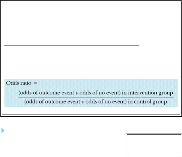
Yet another way of expressing the effect of treatment is the odds ratio. Look back at the two by two table and you will see that the "odds" of dying compared with the odds of surviving for patients in the medical treatment group is 404/921=0.44, and for patients in the surgical group is 350/974=0.36. The ratio of these odds will be 0.36/0.44=0.82.
The general formulas for calculating these "bottom line" effects of an intervention, taken from Sackett and colleagues' latest book,12 are shown in the box.
The outcome event can be desirable (cure, for example) or undesirable (an adverse drug reaction). In the latter case, it is semantically preferable to refer to numbers needed to harm and the relative or absolute increase in risk.
Calculating the "bottom line" effects on an intervention |
|
|
|
|
|
|
|
|
Outcome event |
|
|
|
|
|
|
Group |
Yes |
No |
Total |
Control group |
a |
b |
a+b |
Experimental group |
c |
d |
c+d |
Control event rate (CER)=risk of outcome event in control group=a/(a+b)
Experimental event rate (EER)=risk of outcome event in experimental group=c/(c+d)
Relative risk reduction (RRR)=(CER—EER)/CER
Absolute risk reduction (ARR)=CER—EER
Number needed to treat (NNT)=1/ARR=1/(CER—EER)
Summary
It is possible to be seriously misled by taking the statistical competence (and/or the intellectual honesty) of authors for granted. Some common errors committed (deliberately or inadvertently) by the authors of papers are given in
 Top
Top
 Introduction
 Correlation, regression, and...
 Probability and confidence

the final box. |
The bottom line |
|
Summary |
|
References |
Ten ways to cheat on statistical tests when writing up results
zThrow all your data into a computer and report as significant any relation where P<0.05
zIf baseline differences between the groups favour the intervention group, remember not to adjust for them
zDo not test your data to see if they are normally distributed. If you do, you might get stuck with nonitemmetric tests, which aren't as much fun
zIgnore all withdrawals (drop outs) and non-responders, so the analysis only concerns subjects who fully complied with treatment
zAlways assume that you can plot one set of data against another and calculate an "r value" (Pearson correlation coefficient), and assume that a "significant" r value proves causation
zIf outliers (points which lie a long way from the others on your graph) are messing up your calculations, just rub them out. But if outliers are helping your case, even if they seem to be spurious results, leave them in
zIf the confidence intervals of your result overlap zero difference between the groups, leave them out of your report. Better still, mention them briefly in the text but don't draw them in on the graph— and ignore them when drawing your conclusions
zIf the difference between two groups becomes significant four and a half months into a six month trial, stop the trial and start writing up. Alternatively, if at six months the results are "nearly significant," extend the trial for another three weeks
zIf your results prove uninteresting, ask the computer to go back and see if any particular subgroups behaved differently. You might find that your intervention worked after all in Chinese women aged 52-61
zIf analysing your data the way you plan to does not give the result you wanted, run the figures through a selection of other tests
The articles in this series are excerpts from How to read a paper: the basics of evidence based medicine. The book includes chapters on searching the literature and implementing evidence based findings. It can be ordered from the BMJ Bookshop: tel 0171 383 6185/6245; fax 0171 383 6662. Price £13.95 UK members, £14.95 non-members.
Acknowledgements
I am grateful to Mr John Dobby for educating me on statistics and for repeatedly checking and amending this article. Responsibility for any errors is mine alone.
References
1.Greenhalgh T. Statistics for the non-statistician. I. Different types of data need different statistical tests. BMJ 1997;315:000-0.
2.Bland M. An introduction to medical statistics. Oxford: Oxford University Press, 1987.
 Top
Top
 Introduction
 Correlation, regression, and...
 Probability and confidence

3. Guyatt G, Walter S, Shannon H, Cook D, Jaenschke R, Heddle, N.
Basic statistics for clinicians: 4. Correlation and regression. Can Med Assoc J 1995;152:497-504. [Abstract]
4. Haines A. Multi-practice research: a cohort study. In: Jones R,
Kinmonth AL, eds. Critical reading for primary care. Oxford: Oxford University Press, 1995:124. (Originally published as: Bradford Hill A. The environment and disease: association or causation? Proc R Soc Med 1965;58:295-300.)
5. Altman D. Practical statistics for medical research. London: Chapman and Hall, 1995:210-2.
6. Pocock SJ, Geller XPL, Tsiatis AA. The analysis of multiple endpoints in clinical trials. Biometrics 1987;43:487-98.
7. Guyatt G, Jaenschke R, Heddle, N, Cook D, Shannon H, Walter S. Basic statistics for clinicians. 1. Hypothesis testing. Can Med Assoc J 1995;152:27-32.
8. Gardner MJ, Altman DG, eds. Statistics with confidence: confidence intervals and statistical guidelines.
London: BMJ Books, 1989.
9. Guyatt G, Jaenschke R, Heddle, N, Cook D, Shannon H, Walter S. Basic statistics for clinicians. 2. Interpreting study results: confidence intervals. Can Med Assoc J 1995;152:169-73. [Abstract]
10. Fahey T, Griffiths S, Peters TJ. Evidence based purchasing: understanding the results of clinical trials and systematic reviews. BMJ 1995; 311:1056-60.
11. Yusuf S, Zucker D, Peduzzi P, Liher LD, Takaro T, Kennedy WJ, et al. Effect of coronary artery bypass surgery on survival: overview of ten year results form randomized trials by the coronary artery surgery triallists collaboration. Lancet 1994;344:563-70.
12. Sackett DL, Richardson WS, Rosenberg WMC, Haynes RB. Evidence-based medicine: how to practice and teach EBM. London: Churchill-Livingstone, 1996.
This article has been cited by other articles: (Search Google Scholar for Other Citing
Articles)
M. Eriksson and B. Lindstrom
Validity of Antonovsky's sense of coherence scale: a systematic review
J. Epidemiol. Community Health, June 1, 2005; 59(6): 460 - 466. [Abstract] [Full Text] [PDF]
A. C. Redmond and A.-M. Keenan
Understanding Statistics: Putting P-Values into Perspective
J Am Podiatr Med Assoc, May 1, 2002; 92(5): 297 - 305. [Abstract] [Full Text] [PDF]
W-C Leung
Balancing statistical and clinical significance in evaluating treatment effects
Postgrad. Med. J., March 1, 2001; 77(905): 201 - 204. [Full Text]
This article
Extract 
Respond to this article
Alert me when this article is cited
Alert me when responses are posted
Alert me when a correction is posted
View citation map

Services
Email this article to a friend
Find similar articles in BMJ
Find similar articles in PubMed
Add article to my folders
Download to citation manager
Google Scholar
Articles by Greenhalgh, T.
Articles citing this Article
PubMed
PubMed Citation
Articles by Greenhalgh, T.
Home |
Help |
Search |
Archive |
Feedback |
Table of Contents |
© 1997 BMJ Publishing Group Ltd