Chapter 2 Elements of the Field Theory

2.1 Scalar field. Directional derivative. Gradient.

We say that there is a scalar field defined in space if the value of the quantity is specified at each point of space, i.e. . Let the Cartesian coordinate system in space be given. Then a stationary scalar field can be regarded as a function .

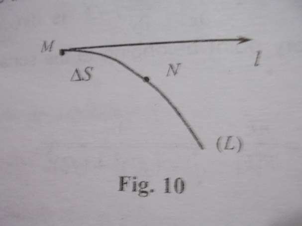
Suppose that a curve starts at the point in the direction (see Fig. 10)

Then the rate of change of the field in this direction (related to unit length) is called the derivative of along the direction :

To compute the directional derivative let us suppose that the curve is represented in parametrical form by the equation where the parameter is the arc length reckoned along . Then the values of taken along from a composite function . Therefore, by the rule of differentiating a composite function, we have

The right-hand side can be represented as a scalar product of two vectors. The first vector is called the gradient of the field. It is designed as .

The second vector is the unit vector in the direction . Thus (*)( denotes the projection of the gradient on the axis passing the direction ).

Note that the derivative , and are also directional derivatives, for instance is the derivative in the direction of the x-axis.

Let us put down one more useful formula containing the gradient which is based on the definition of the total differential

.

Let the field and a point be given. Let us set the following problem: in what direction is the derivative maximal? We see that on the basic of the formula (*) the problem reduces to the following question in which direction is the projection of the vector maximal? Evidently, the maximal projection of any vector is obtained when we take its own direction, the maximal projection being equal to the modulus of the vector.

Thus the vector at the point indicates the direction of the maximal rate of increase of the field ; this maximal rate (related to the unit length) is being equal to .

2.2. Level surface.

Level surface of a field u(M) are the surface on which the field assumes constant value, that is the surface represented by equation of the form: u(M)=const

Depending on the physical meaning of the field these surface may be called isothermic surfaces (for the temperature field), isobaric surfaces and the like.

There is a simple relationship between these surfaces and the gradient of the field: at each point M the gradient is normal to the level surface passing through the point M.

Actually as it seen on Fig. 11, the surface u=C and u=C+ΔC can be regarded as being almost plane near the point M if ΔC is sufficiently small, and besides

But it is clear that if l directly along the normal to the surface the quantity ΔS will assume its least value, and will therefore assume its maximal value. This implies our assertion.

In particular, we see that the assertion enables us to solve the following problem: to find the equation of the tangent plane passing through a point M₀ (x₀, y₀, z₀) of a surface (L) having an equation of the form F(x, y, z)=0. To solve the problem let us introduce a scalar field by means of the equation u=F(x, y, z). Then (L) becomes one of the level surfaces of the field because we have u=F(x, y, z)=0 on the surface.

Then the vector (the subscript “zero” indicates that the corresponding derivatives are taken at the point M₀) is perpendicular to the sought-for tangent plane.

Hence, we obtain the equation of the plane:

The last equation can be put down as dF=0.

A surface for which the tangent plane is to be constructed can be represented by an equation of the form z=f(x, y). Here we can rewrite the equation as z-f(x, y)=0 and denote its left hand side by F(x, y, z). Then the last formula for a plane is directly applicable, and thus we have

i.e.

The right-hand side is equal to the total differential df, we thus obtain the geometrical meaning of the total differential of a function of two independent variables. Namely, the differential is equal to the increment of the third coordinate of the point in the tangent plane .

Take an example. Let us compute the gradient of a centrally symmetric field u=f(r) where . In this case, the level surfaces are concentric spheres with center at the origin of coordinates. If we take two spheres for which the difference of their radii is equal to dr then the difference of the corresponding values of the function f which are taken on these surfaces will be equal to df .

Therefore, the change rate of the function in a direction, which is transversal to the level surfaces, (that is along a radius) is equal to . Hence,

where is the unit vector in the direction of the vector .

Let the reader obtain this result on the basic of the definition