1 .5. Integral over an arbitrary plane region.

Let the domain of integration be an arbitrary plane figure lying in the x, y-plane. For instance, take the domain depicted in Fig. 3.

The consideration given above can be transferred to this case with some slight changes. Namely, instead of the integral (1) we arrive at an integral of the form

,

where y=y₁=₁(x) and y=y₂=₂(x) are, respectively, the equations of the upper and lower parts of the boundary of the domain. Accordingly, the final result will be of the form:

.

Consequently, the limits of integration in the inner integral are variable in the general case; they depend on the variable of integration in the outer integral.

We can also invert the order of integration. That is perform the first integration with respect to x and the second – with respect to y. Then we arrive at a formula of the form

.

It is sometimes necessary to break the domain of integration into several parts before setting up the limits of integration.

For example, .

1.6. Integral over a three-dimensional region.

Let us now consider an integral , where is a solid, that is a domain in space.

We compute it following the procedure, which was developed for an integral over a plane figure. The corresponding integral sum is now represented as an iterated three-fold sum. In the simplest case when is a rectangular parallelepiped defined by the inequalities , and we obtain, after passing to the limit in the integral sum, the formula .

By the way, it is possible to perform here the integration by inverting the order of integration in five different ways because there are six different combinations (permutation) of the differentials .

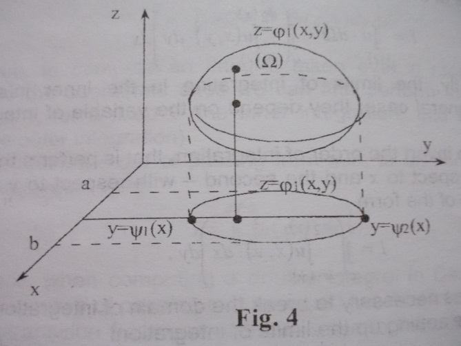
If the domain of the integration is of more general form the determination of the limits of the integration could be more complicated.

Let the domain of integration be of the form shown in Fig.4. Then we can put down integral in the form: .

1.7. Passing to polar coordinates in plane.

As in the case of one-dimensional integral, we can introduce different variables of integration while computing a double integral. Here we shall consider a typical example of computing a double integral in the polar coordinates.

The polar coordinate system is a two-dimentional coordinate system in which each point on a plane is determined by a distance  from a fixed point and an angle (or sometimes ) from a fixed direction.

The fixed point (analogous to the origin of a Cartesian system) is called the pole, and the ray from the pole in the fixed direction is the polar axis. The distance from the pole is called the radial coordinate or radius, and the angle is the angular coordinate, polar angle, or azimuth.

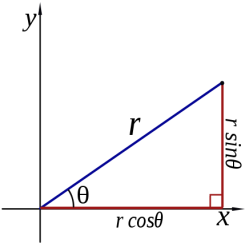
The polar coordinates r and φ can be converted to the Cartesian coordinates x and y by using the trigonometric functions sine and cosine:

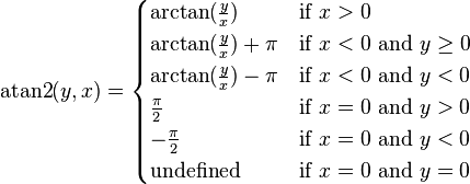
The Cartesian coordinates x and y can be converted to polar coordinates r and φ with r ≥ 0 and φ in the interval (−π, π] by:

 (as in the Pythagorean theorem), and

,

where atan2 is a common variation on the arctangent function defined as

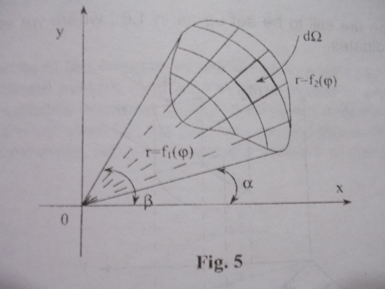Let us take an integral of the form: , where is a region in the - plane, which is depicted in Fig.5. It is necessary to perform the integration in polar coordinates. We must divide the domain into parts by means of the coordinate curves of the polar coordinate system, i.e. by lines and , as it is shown in Fig.5.

Each of the elementary areas thus obtained can be regarded as being equal to a rectangle with sides and to within infinitesimals of higher order. Hence, we have . Performing the summation over all the elementary areas we obtain , where the integrand must of course be expressed as a function of and . By analogy with 1.4.-1.5., we set up the limits of integration and thus receive . The geometrical meaning of the limits of integration is illustrated in Fig.5.

Note, that polar coordinates are particularly convenient for regions whose boundary consists of coordinate curves of the polar coordinate system.

1.8. Passing to cylindrical and spherical coordinates.

Let us take an integral , where is a domain in space. It is necessary to perform the integration in cylindrical coordinates. We have to divide the domain into parts by means of the coordinate surfaces of the cylindrical coordinate system, i.e. the surfaces , and .

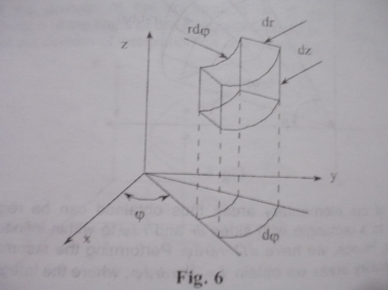
Then each of the elements of volume (see Fig.6.) can be regarded as being equal to the volume of the rectangular parallelepiped with dimensions , and to within infinitesimals of higher order of smallness (relative to the element of volume). Consequently we have . Dependence between Cartesian system and cylindrical system can be written in the form: . Therefore the integral takes the form where the limits of integration are still to be set up as in previous point.

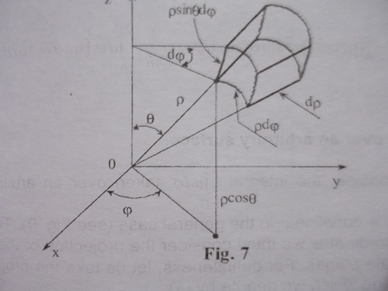
Let we use spherical coordinates.

(надо добавить о системе координат)

The element of volume can be again regarded as being approximately equal to the volume of the corresponding rectangular parallelepiped (see Fig.7.). In this case the rectangular parallelepiped has the sides , and . Dependence between Cartesian system and spherical system can be written in the form: . Thus we have and . (*)

The limits of the integration are set up in a particularly simple manner in this coordinate system (and also in other systems) when consists of coordinate surfaces because in such a case not only the limits of the outer integration are constants but the first and second integrations as well.

1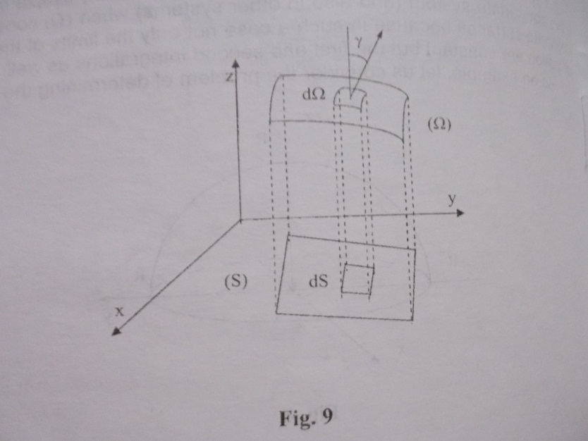 .9. Integral over arbitrary surface.

Let us consider the integral taken over an arbitrary surface , which can be curvilinear in the general case (see Fig.9). To compute it in Cartesian coordinates we must consider the projection of the surface on the coordinate planes. For definiteness, let us take the projection of on the - plane which we denote by .

Since the element (the area of an infinitesimal part) of a curvilinear surface can be regarded as being plane to within infinitesimal of higher order of smallness relative to the area, we have where and is a normal vector. It follows that . Let the surface in question be represented by an equation of the form . Then the vector is directed along the normal to the surface at every point belonging to the surface. Hence we have: . Therefore, In particular case we derive the formula for the area . For the case of projecting on planes and formulas will be similarly obtained.

1.10. Curvilinear integral.