

1.3. Geometrical meaning of an integral over a plane region.
Such an integral, unlike other multiple integrals, can be directly interpreted geometrically. Its geometric meaning is similar to that of an ordinary define integral.
 Let
us be given an integral of the form
Let
us be given an integral of the form
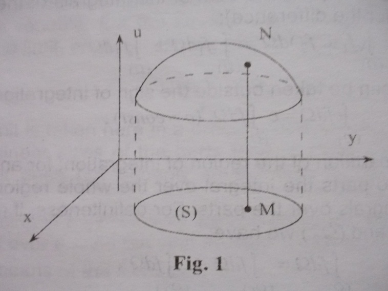
 , where (S)
is a domain lying in a plane. (See Fig. 1.). Let us draw the u-axis
perpendicularly to the plane and construct a line segment of length
ƒ(M) parallel to the u-axis
and passing through a point M
belonging to the domain (S).
, where (S)
is a domain lying in a plane. (See Fig. 1.). Let us draw the u-axis
perpendicularly to the plane and construct a line segment of length
ƒ(M) parallel to the u-axis
and passing through a point M
belonging to the domain (S).
For simplicity’s sake we now consider positive values of ƒ; then the segment is drawn in the positive direction of the u-axis and the end-point N of the segment lies above the plane P. When the point M runs throughout the domain (S) the corresponding point N describe a surface, which is the graph of integrand. The surface together with the plane figure (S) and cylindrical surface formed by the line segment parallel to the u-axis and drawn through each point of the contour bordering the domain (S) bound a cylindrical body.
The
geometric meaning of integral
 lies in the fact that it is equal to the volume of the cylindrical
body. Indeed, the element of volume corresponding to a plane element
dS of the
domain (S)
containing a point M
can be regarded as a right cylinder with base dS
and height ƒ(M)
to within infinitesimals of higher order. Hence, this is
approximately equal to
lies in the fact that it is equal to the volume of the cylindrical
body. Indeed, the element of volume corresponding to a plane element
dS of the
domain (S)
containing a point M
can be regarded as a right cylinder with base dS
and height ƒ(M)
to within infinitesimals of higher order. Hence, this is
approximately equal to .
Summing up these elements of volume we arrive at the formula
.
Summing up these elements of volume we arrive at the formula

which as what set up to prove.
1.4. Integrals over a rectangle.
We
now consider an integral
 where (Ω)
is a rectangle bounded by coordinate lines of the Cartesian
coordinate system arbitrary chosen in a plane (see Fig2). The
rectangle is described by inequalities a
≤ x ≤ b and c ≤y ≤ d where a,
b, c , d are some constants. When
forming an integral sum it is natural to break up (Ω)
into parts by means of straight lines
parallel to the coordinate axes which divide the integral a
≤ x ≤ b into parts ∆xi
and the integral c
≤y ≤ d into parts
∆yi.
where (Ω)
is a rectangle bounded by coordinate lines of the Cartesian
coordinate system arbitrary chosen in a plane (see Fig2). The
rectangle is described by inequalities a
≤ x ≤ b and c ≤y ≤ d where a,
b, c , d are some constants. When
forming an integral sum it is natural to break up (Ω)
into parts by means of straight lines
parallel to the coordinate axes which divide the integral a
≤ x ≤ b into parts ∆xi
and the integral c
≤y ≤ d into parts
∆yi.
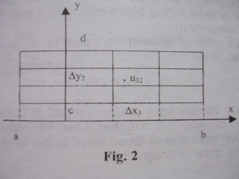 Let
us denote by uik
the value of the integrant u=u(x, y)
at a point belonging to the subregion adjoining the intersection of
the i- th
vertical line with the k-th
horizontal line (see Fig. 2).
Let
us denote by uik
the value of the integrant u=u(x, y)
at a point belonging to the subregion adjoining the intersection of
the i- th
vertical line with the k-th
horizontal line (see Fig. 2).
We
then approximately have
 where the summation is extended over all the subregions. It is a
two-dimensional integral sum:
where the summation is extended over all the subregions. It is a
two-dimensional integral sum:
 .
.
If the divisions along the y-axis are sufficiently small the sum inside the brackets is close to the corresponding integral:
 .
.
It follows that
 .
(1)
.
(1)
But this also an integral sum for function, which depends on x. Hence, if the divisions along the x-axis are also sufficiently small, we can write:
 .
(2)
.
(2)
In the process of decreasing the subregions of the partitions equalities (1) and (2) become more and still more accurate and turn into the precise relations in the limit. Consequently,
 .
.
Thus, to compute an integral taken over a rectangle with sides parallel to the coordinate axes we can first perform the integration with respect to y, for a fixed x ( the inner integration) and then integrate the result ( the outer integration).
The reverse order of passing from sum to an iterated two-fold sum (see above) would yield:

Hence, when computing a double integral in Cartesian coordinates we have two ways of passing to a repeated two-fold integral.
The transition from one of these ways to other is referred to as the inversion of the order of integration.