

Work procedure
1. Fill in tank 1 with water.
2. Open faucet 6 on 1/4 - 1/5 turnover and set a low water rate through Venturi’s flow meter.
3. Measure loss in pressure between cross- sections 1-1 and 2-2.
4. Measure volume of water W in calibrated tank 5 and time T for its filling.
5. Change position of faucet 6. Repeat the procedures mentioned above for other flow rate capacities. The obtained results put down in Table 5.1.
6. Estimate actual and theoretical flow rates.
7. Calculate calibration coefficient k, flow rate coefficient and coefficient of resistance .
8.
Basing on receiving results build the diagram showing the relation
between the actual flow rate and water head
![]() for Venturi’s flow meters.
for Venturi’s flow meters.
9.
Repeat procedures 2 - 8 for the diaphragm and the nozzle, fill in the
tables
and build diagrams
![]() .
.
Table 5.1
Number of measurement |
1 |
2 |
3 |
4 |
5 |
Water head H, cm |
|
|
|
|
|
Time for measured tank filling T, s |
|
|
|
|
|
Measured volume W, cm3 |
|
|
|
|
|
Actual flow rate Qr, cm3/s |
|
|
|
|
|
Calibration coefficient k |
|
|
|
|
|
Theoretical flow rate QT , cm3/s |
|
|
|
|
|
Losses on Tube, ΔH cm |
|
|
|
|
|
Resist. coef., ζ |
|
|
|
|
|
Rate coefficient, μ |
|
|
|
|
|
Laboratory work 6 centrifugal pump testing Brief theoretical information
Centrifugal pumps are widely spread due to simple design, comparatively small size and high efficiency, smooth liquid supply and other advantages.
Main operating part of the pump is an impeller (Fig. 6.1). It rotates and raises pressure of filled liquid and with increased speed swirls it in a spiral chamber. Transformation of power of the driven mechanism to power of the flow occurs as a result of power interaction of impeller and liquid flow. The volute casing directs the liquid to the pump outlet, where the kinetic energy of the liquid is partly converted into the energy of pressure.

Fig. 6.1. Scheme of centrifugal pump: 1 is impeller; 2 is spiral chamber
Pressure head of water being discharged can be obtained by means of Bernoulli’s equation for cross-sections at entry and exit of the impeller.
![]() .
.
Applying to the device (Fig. 6.2) we get:
![]() ,
,
where h0 is distance between points of manometer connection 5 and vacuum-gauge 4; PH is manometer pressure at exit; PV is vacuum at entrance; VM is speed in discharge pipe 6; VV is speed in suction pipe 3.
On the other hand, pressure of pump 2 can be defined as difference of specific energy received by pump from the engine for each kilogram of liquid and part of energy lost in pump due to hydraulic and mechanical resistance.
Lost part of energy can be determined by efficiency of the pump:
![]()
Considering
that
![]() g,
one receive the formula for a pump head:
g,
one receive the formula for a pump head:
![]()

Fig. 6.2. Scheme of experimental system for centrifugal pump testing
Power of electric motor 1 can be determined by torsion balance 11
![]()
where G0 is the torsion balance weight; L is arm of the torsion balance; n is the number of circles of an electric motor.
After putting value of pressure into formula we get general equation for HP=(Q, n). As usual the pumps operate with uniform speed. Therefore the characteristics of this pump will be the following: n = const, HP=(Q).
Data received analytically omit hydraulic and mechanical losses in the pump, therefore they are determined experimentally. Experimental pump characteristics are received by steady pump operation upon the pipeline.
Graphically liquid rate and pressure head for steady-state regime are determined by pump operating point, that is the intersection of conduit and pump characteristics (Fig. 6.3).
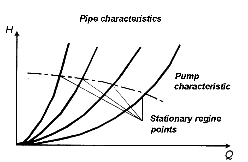
Fig. 6.3. Graphical description of centrifugal pump
Consequently, any amount of points relating to stationary operation can be obtained by changing hydraulic resistance of the conduit. The pump characteristics can be received by drawing a curve over these points HP=(Q), (Fig. 6.3). Efficiency of the pump can be determined by measuring the power at the motor shaft:
![]() .
.