

Efficient estimator.
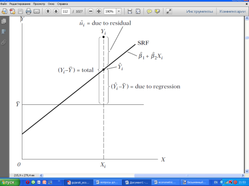
30) Break down the variation of Yi into two components. Illustrate. (Figure 3.10 p. 83).
31) What is spurious (or nonsense) regression? What does this imply for regression analysis? (pp. 806–807)
To see why stationary time series are so important, consider the following two
random walk models:
Yt = Yt−1 + ut
Xt = Xt−1 + vt
where we generated 500 observations of ut from ut ∼ N(0, 1) and 500 observations
of vt from vt ∼ N(0, 1) and assumed that the initial values of both Y
and X were zero. We also assumed that ut and vt are serially uncorrelated as
well as mutually uncorrelated. As you know by now, both these time series
are nonstationary; that is, they are I(1) or exhibit stochastic trends.
the phenomenon of spurious or nonsense
regression, first discovered by Yule.17 Yule showed that (spurious)
correlation could persist in nonstationary time series even if the sample is
very large. That there is something wrong in the preceding regression is suggested
by the extremely low Durbin–Watson d value, which suggests very strong first-order autocorrelation. According to Granger and Newbold, an
R2 > d is a good rule of thumb to suspect that the estimated regression is spurious,
as in the example above.
32) X2 and X3 are collinear. What does this mean? (pp. 203–204)
λ2 X2i + λ3 X3i = 0
If such an exact linear relationship exists, then X2 and X3 are said to be collinear or linearly dependent. On the other hand, if (7.1.8) holds true only when λ2 = λ3 = 0, then X2 and X3 are said to be linearly independent.
Thus, if X2i = −4X3i or X2i + 4X3i = 0
the two variables are linearly dependent, and if both are included in a regression model, we will have perfect collinearity or an exact linear relation- ship between the two regressors. Suppose that in (7.1.1) Y, X2, and X3 represent consumption expenditure, income, and wealth of the consumer, respectively. In postulating that consumption expenditure is linearly related to income and wealth, economic theory presumes that wealth and income may have some independent influence on consumption. If not, there is no sense in including both income and wealth variables in the model. In the ex-treme, if there is an exact linear relationship between income and wealth, we have only one independent variable, not two, and there is no way to assess the separate influence of income and wealth on consumption.
33) Interpret the coefficients of equation (p. 214).
Let us now interpret these regression coefficients: −0.0056 is the partial
regression coefficient of PGNP and tells us that with the influence of FLR
held constant, as PGNP increases, say, by a dollar, on average, child mortality
goes down by 0.0056 units. To make it more economically interpretable,
if the per capita GNP goes up by a thousand dollars, on average, the number
of deaths of children under age 5 goes down by about 5.6 per thousand live
births. The coefficient −2.2316 tells us that holding the influence of PGNP
constant, on average, the number of deaths of children under 5 goes down by
about 2.23 per thousand live births as the female literacy rate increases by
one percentage point. The intercept value of about 263, mechanically interpreted,
means that if the values of PGNP and FLR rate were fixed at zero, the
mean child mortality would be about 263 deaths per thousand live births. Of
course, such an interpretation should be taken with a grain of salt. All one
could infer is that if the two regressors were fixed at zero, child mortality will
be quite high, which makes practical sense. The R2 value of about 0.71
means that about 71 percent of the variation in child mortality is explained
by PGNP and FLR, a fairly high value considering that the maximum value
of R2 can at most be 1. All told, the regression results make sense.
CMi = β1 + β2PGNPi + β3FLRi + ui
CM-child mortality; PGNP-per capita GNP; FLR-female literacy rate;
34) Why is the method of generalized least squares (see previous question) also called weighted least squares? Illustrate in a diagram. (pp. 397–398)
In OLS we minimize _uˆi2 =_(Yi −βˆ1 −βˆ2Xi)2
but in GLS we minimize the expression which can also be written as
_wiuˆi2 =_wi(Yi −βˆ1*X0i −βˆ2*Xi)2
where wi = 1/σi2 [verify that (11.3.11) and (11.3.7) are identical]. Thus, in GLS we minimize a weighted sum of residual squares with wi = 1/σi2 acting as the weights, but in OLS we minimize an unweighted or (what amounts to the same thing) equally weighted RSS.
In the (unweighted) OLS, each uˆi2 associated with points A, B, and C will
receive the same weight in minimizing the RSS. Obviously, in this case the uˆi2 associated with point C will dominate the RSS. But in GLS the ex- treme observation C will get relatively smaller weight than the other two observations.