

Consequences of Micronumerosity
In a parody of the consequences of multicollinearity, and in a tongue-incheek
manner, Goldberger cites exactly similar consequences of micronumerosity,
that is, analysis based on small sample size.15 The reader is
advised to read Goldberger’s analysis to see why he regards micronumerosity
as being as important as multicollinearity.
14. Give three ways to detect multicollinearity (1, 2, 6—Variance Inflation Factor only). Briefly explain. (pp. 359–363)
1. High R2 but few significant t ratios. As noted, this is the “classic”
symptom of multicollinearity. If R2 is high, say, in excess of 0.8, the F test in
most cases will reject the hypothesis that the partial slope coefficients are
simultaneously equal to zero, but the individual t tests will show that none or
very few of the partial slope coefficients are statistically different from zero.
This fact was clearly demonstrated by our consumption–income–wealth
example.
Although this diagnostic is sensible, its disadvantage is that “it is too
strong in the sense that multicollinearity is considered as harmful only
when all of the influences of the explanatory variables on Y cannot be disentangled.”
18
2. High pair-wise correlations among regressors. Another suggested
rule of thumb is that if the pair-wise or zero-order correlation coefficient between
two regressors is high, say, in excess of 0.8, then multicollinearity is a
serious problem. The problem with this criterion is that, although high
zero-order correlations may suggest collinearity, it is not necessary that they
be high to have collinearity in any specific case. To put the matter somewhat
technically, high zero-order correlations are a sufficient but not a necessary
condition for the existence of multicollinearity because it can exist even
though the zero-order or simple correlations are comparatively low (say, less
than 0.50). To see this relationship, suppose we have a four-variable model:
Yi = β1 + β2X2i + β3X3i + β4X4i + ui
and suppose that
X4i = λ2X2i + λ3X3i
where λ2 and λ3 are constants, not both zero. Obviously, X4 is an exact linear
combination of X2 and X3, giving R2= 1, the coefficient of determination
in the regression of X4 on X2 and X3.
6. Tolerance and variance inflation factor. We have already introduced
TOL and VIF. As R2j
, the coefficient of determination in the regression
of regressor Xj on the remaining regressors in the model, increases toward
unity, that is, as the collinearity of Xj with the other regressors increases,
VIF also increases and in the limit it can be infinite.
Some authors therefore use the VIF as an indicator of multicollinearity.
The larger the value of VIFj, the more “troublesome” or collinear the variable
Xj. As a rule of thumb, if the VIF of a variable exceeds 10, which will
happen if R2j
exceeds 0.90, that variable is said be highly collinear.27
Of course, one could use TOLj as a measure of multicollinearity in view
of its intimate connection with VIFj. The closer is TOLj to zero, the greater
the degree of collinearity of that variable with the other regressors. On the other hand, the closer TOLj is to 1, the greater the evidence that Xj is not
collinear with the other regressors.
VIF (or tolerance) as a measure of collinearity is not free of criticism. As
(10.5.4) shows, var ( ˆ βj ) depends on three factors: σ2,
_
x2
j , and VIFj. A high
VIF can be counterbalanced by a low σ2 or a high
_
x2
j . To put it differently,
a high VIF is neither necessary nor sufficient to get high variances and high
standard errors. Therefore, high multicollinearity, as measured by a high
VIF, may not necessarily cause high standard errors. In all this discussion,
the terms high and low are used in a relative sense.
To conclude our discussion of detecting multicollinearity, we stress that
the various methods we have discussed are essentially in the nature of
“fishing expeditions,” for we cannot tell which of these methods will work in
any particular application. Alas, not much can be done about it, for multicollinearity
is specific to a given sample over which the researcher may not
have much control, especially if the data are nonexperimental in nature—
the usual fate of researchers in the social sciences.
Again as a parody of multicollinearity, Goldberger cites numerous ways of
detecting micronumerosity, such as developing critical values of the sample
size, n*, such that micronumerosity is a problem only if the actual sample
size, n, is smaller than n*. The point of Goldberger’s parody is to emphasize
that small sample size and lack of variability in the explanatory variables may
cause problems that are at least as serious as those due to multicollinearity.
15. Illustrate the nature of homoscedasticity and heteroscedasticity in two diagrams. (pp. 387–388).
16.Give three (out of seven) reasons for heteroscedasticity. Briefly explain. (pp. 389–393)
As noted in Chapter 3, one of the important assumptions of the classical
linear regression model is that the variance of each disturbance term ui ,
conditional on the chosen values of the explanatory variables, is some constant
number equal to σ2. This is the assumption of homoscedasticity, or
equal (homo) spread (scedasticity), that is, equal variance. Symbolically,
Diagrammatically, in the two-variable regression model homoscedasticity
can be shown as in Figure 3.4, which, for convenience, is reproduced as
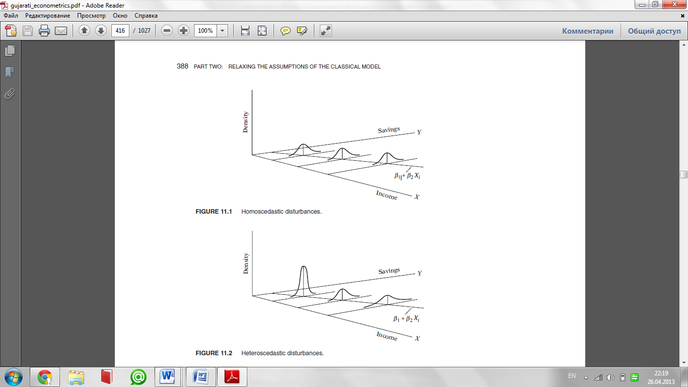
Figure 11.1. As Figure 11.1 shows, the conditional variance of Yi (which is
equal to that of ui), conditional upon the given Xi, remains the same regardless
of the values taken by the variable X.
In contrast, consider Figure 11.2, which shows that the conditional variance
of Yi increases as X increases. Here, the variances of Yi are not the
same. Hence, there is heteroscedasticity. Symbolically,
Notice the subscript of σ2, which reminds us that the conditional variances
of ui (= conditional variances of Yi) are no longer constant.
To make the difference between homoscedasticity and heteroscedasticity
clear, assume that in the two-variable model Yi = β1 + β2Xi + ui , Y represents
savings and X represents income. Figures 11.1 and 11.2 show that as
income increases, savings on the average also increase. But in Figure 11.1 the variance of savings remains the same at all levels of income, whereas in
Figure 11.2 it increases with income. It seems that in Figure 11.2 the higherincome
families on the average save more than the lower-income families,
but there is also more variability in their savings.
There are several reasons why the variances of ui may be variable, some
of which are as follows.1
1. Following the error-learning models, as people learn, their errors of behavior
become smaller over time. In this case, σ2
i is expected to decrease. As
an example, consider Figure 11.3, which relates the number of typing errors
made in a given time period on a test to the hours put in typing practice. As
Figure 11.3 shows, as the number of hours of typing practice increases, the
average number of typing errors as well as their variances decreases.
2. As incomes grow, people have more discretionary income2 and hence
more scope for choice about the disposition of their income. Hence, σ2
i is
likely to increase with income. Thus in the regression of savings on income
one is likely to find σ2
i increasing with income (as in Figure 11.2) because
people have more choices about their savings behavior. Similarly, companies
with larger profits are generally expected to show greater variability
in their dividend policies than companies with lower profits. Also, growthoriented
companies are likely to show more variability in their dividend
payout ratio than established companies.
3. As data collecting techniques improve, σ2
i is likely to decrease. Thus,
banks that have sophisticated data processing equipment are likely to commit fewer errors in the monthly or quarterly statements of their customers
than banks without such facilities.
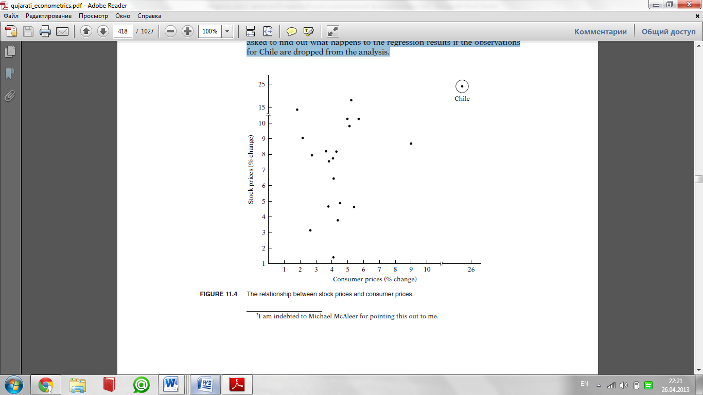
4. Heteroscedasticity can also arise as a result of the presence of outliers.
An outlying observation, or outlier, is an observation that is much different
(either very small or very large) in relation to the observations in the
sample. More precisely, an outlier is an observation from a different population
to that generating the remaining sample observations.3 The inclusion
or exclusion of such an observation, especially if the sample size is small,
can substantially alter the results of regression analysis.
As an example, consider the scattergram given in Figure 11.4. Based on the
data given in exercise 11.22, this figure plots percent rate of change of stock
prices (Y) and consumer prices (X) for the post–WorldWar II period through
1969 for 20 countries. In this figure the observation on Y and X for Chile can
be regarded as an outlier because the given Y and X values are much larger
than for the rest of the countries. In situations such as this, it would be hard
to maintain the assumption of homoscedasticity. In exercise 11.22, you are
asked to find out what happens to the regression results if the observations
for Chile are dropped from the analysis.
5. Another source of heteroscedasticity arises from violating Assumption
9 of CLRM, namely, that the regression model is correctly specified.
Although we will discuss the topic of specification errors more fully in
Chapter 13, very often what looks like heteroscedasticity may be due to the
fact that some important variables are omitted from the model. Thus, in the
demand function for a commodity, if we do not include the prices of commodities
complementary to or competing with the commodity in question
(the omitted variable bias), the residuals obtained from the regression may
give the distinct impression that the error variance may not be constant. But
if the omitted variables are included in the model, that impression may
disappear.
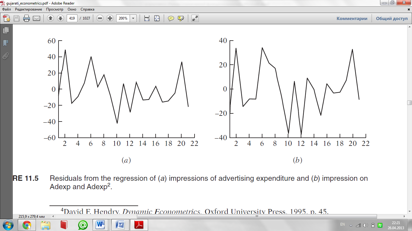
As a concrete example, recall our study of advertising impressions retained
(Y) in relation to advertising expenditure (X). (See exercise 8.32.) If
you regress Y on X only and observe the residuals from this regression, you
will see one pattern, but if you regress Y on X and X2, you will see another
pattern, which can be seen clearly from Figure 11.5. We have already seen
that X2 belongs in the model. (See exercise 8.32.)
6. Another source of heteroscedasticity is skewness in the distribution
of one or more regressors included in the model. Examples are economic
variables such as income, wealth, and education. It is well known that the
distribution of income and wealth in most societies is uneven, with the bulk
of the income and wealth being owned by a few at the top.
7. Other sources of heteroscedasticity: As David Hendry notes, heteroscedasticity
can also arise because of (1) incorrect data transformation
(e.g., ratio or first difference transformations) and (2) incorrect functional
form (e.g., linear versus log–linear models).4
Note that the problem of heteroscedasticity is likely to be more common
in cross-sectional than in time series data. In cross-sectional data, one
usually deals with members of a population at a given point in time, such as
individual consumers or their families, firms, industries, or geographical
subdivisions such as state, country, city, etc. Moreover, these members may
be of different sizes, such as small, medium, or large firms or low, medium,
or high income. In time series data, on the other hand, the variables tend to
be of similar orders of magnitude because one generally collects the data for
the same entity over a period of time. Examples are GNP, consumption
expenditure, savings, or employment in the United States, say, for the period
1950 to 2000.
As an illustration of heteroscedasticity likely to be encountered in crosssectional
analysis, consider Table 11.1. This table gives data on compensation
per employee in 10 nondurable goods manufacturing industries, classified
by the employment size of the firm or the establishment for the year
1958. Also given in the table are average productivity figures for nine
employment classes.
17) What happens to ordinary least squares estimators and their variances in the presence of heteroscedasticity? (pp. 393–394, 442)
1. Following the error-learning models, as people learn, their errors of behavior
become smaller over time. In this case, σ2 i is expected to decrease.
2. As incomes grow, people have more discretionary income2 and hence
more scope for choice about the disposition of their income. Hence, σ2
i is likely to increase with income. Thus in the regression of savings on income
one is likely to find σ2 i increasing with income because people have more choices about their savings behavior.
4. Heteroscedasticity can also arise as a result of the presence of outliers.
An outlying observation, or outlier, is an observation that is much different
(either very small or very large) in relation to the observations in the
sample.
6. Another source of heteroscedasticity is skewness in the distribution
of one or more regressors included in the model. Examples are economic
variables such as income, wealth, and education.
18) How can you informally detect heteroscedasticity? (pp. 401–403)
Informal Methods
Nature of the Problem Very often the nature of the problem under
consideration suggests whether heteroscedasticity is likely to be encountered.
For example, following the pioneering work of Prais and Houthakker
on family budget studies, where they found that the residual variance
around the regression of consumption on income increased with income,
one now generally assumes that in similar surveys one can expect unequal
variances among the disturbances.
Graphical Method If there is no a priori or empirical information
about the nature of heteroscedasticity, in practice one can do the regression
analysis on the assumption that there is no heteroscedasticity and then do a
postmortem examination of the residual squared ˆu2 i to see if they exhibit any systematic pattern.
19) Explain the intuition of the Goldfeld-Quandt test for heteroscedasticity using a sketch of the scatterplot for Xi and Yi (pp. 408–410). What are the drawbacks of this test?
Goldfeld-Quandt Test.17 This popular method is applicable if one assumes
that the heteroscedastic variance, σ2 i , is positively related to one of the explanatory variables in the regression model. For simplicity, consider the usual two-variable model:
Yi = β1 + β2Xi + ui
Step 1. Order or rank the observations according to the values of Xi, beginning
with the lowest X value.
Step 2. Omit c central observations, where c is specified a priori, and
divide the remaining (n − c) observations into two groups each of (n − c)/ 2 observations.
Step 3. Fit separate OLS regressions to the first (n − c)/ 2 observations
and the last (n − c)/ 2 observations, and obtain the respective residual sums
of squares RSS1 and RSS2, RSS1 representing the RSS from the regression
corresponding to the smaller Xi values (the small variance group) and RSS2
that from the larger Xi values (the large variance group). These RSS each
have
(n− c)/2 –k or _n− c − 2k/df
where k is the number of parameters to be estimated, including the intercept.
(Why?) For the two-variable case k is of course 2.
Step 4. Compute the ratio
λ=(RSS2/df)/ RSS1/df
20) Explain the intuition of the Breusch-Pagan-Godfrey test for heteroscedasticity (pp. 411–412).
Breusch–Pagan–Godfrey Test.The success of the Goldfeld–Quandt
test depends not only on the value of c (the number of central observations
to be omitted) but also on identifying the correct X variable with which to
order the observations. This limitation of this test can be avoided if we
consider the Breusch–Pagan–Godfrey (BPG) test.
To illustrate this test, consider the k-variable linear regression model
Yi = β1 + β2X2i + ·· ·+βkXki + ui
Step 1. Estimate by OLS and obtain the residuals ˆu1, ˆu2, . . . , ˆun.
Step 2. Obtain ˜σ2 = cumma ˆu2/n
i /n. Recall from Chapter 4 that this is the
maximum likelihood (ML) estimator of σ2
Step 3. Construct variables pi defined as
pi = ˆu2/σ2 which is simply each residual squared divided by ˜σ2.
Step 4. Regress pi thus constructed on the Z’s as
pi = α1 + α2Z2i +· · ·+αmZmi + vi where vi is the residual term of this regression.
Step 5. Obtain the ESS (-)=1/2(ESS)
21) What are the advantages of the White test for heteroscedasticity (compared to the Goldfeld-Quandt and Breusch-Pagan-Godfrey tests)? (p. 413).
White’s General Heteroscedasticity Test. Unlike the Goldfeld–
Quandt test, which requires reordering the observations with respect to the
X variable that supposedly caused heteroscedasticity, or the BPG test, which
is sensitive to the normality assumption, the general test of heteroscedasticity
proposed by White does not rely on the normality assumption and is easy
to implement.
A comment is in order regarding the White test. If a model has several
regressors, then introducing all the regressors, their squared (or higherpowered)
terms, and their cross products can quickly consume degrees of freedom.
22) What is the remedial measure for heteroscedasticity when the error variance i (s 2 , )s known? Briefly explain. (pp. 415–416)
When σi2 Is Known: The Method of Weighted Least Squares
If σi2 is known, the most straightforward method of correcting heteroscedasticity is by means of weighted least squares, for the estimators thus obtained are BLUE. To illustrate the method, suppose we want to study the relationship between compensation and employment size. For simplicity, we measure employment size by 1 (1–4 employees), 2 (5–9 employees),..., 9 (1000–2499 employees.
Now letting Y represent average compensation per employee ($) and X the employment size, we run the fol- lowing regression:
Yi /σi = βˆ1∗(1/σi ) + βˆ2∗(Xi /σi ) + (uˆi /σi )
where σi are the standard deviations of wages. As noted earlier, if true σi2 are known, we can use the WLS method to obtain BLUE estimators. Since the true σi2 are rarely known, is there a way of obtaining consistent (in the statistical sense) estimates of the variances and covariances of OLS estimators even if there is heteroscedasticity? The answer is yes.
23) Explain the nature of autocorrelation. Illustrate typical patterns of autocorrelation in a couple of diagrams, and compare to absence of autocorrelation. (pp. 442–444).
The term autocorrelation may be defined as “correlation between mem- bers of series of observations ordered in time [as in time series data] or space [as in cross-sectional data].’’In the regression context, the classical linear regression model assumes that such autocorrelation does not exist in the disturbances ui . Symbolically,
E(ui uj ) = 0 i à= j
For example, if we are dealing with quarterly time series data involving the regression of output on labor and capital inputs and if, say, there is a labor strike affecting output in one quarter, there is no reason to believe that this disruption will be carried over to the next quarter. That is, if output is lower this quarter, there is no reason to expect it to be lower next quarter. Similarly, if we are dealing with cross-sectional data involving the regression of family consumption expenditure on family income, the effect of an increase of one family’s income on its consumption expenditure is not expected to affect the consumption expenditure of another family.