

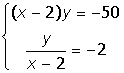
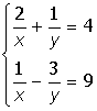
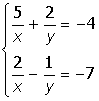
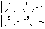
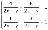
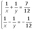
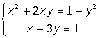
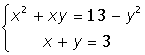
6. Solve the system of equations
1. |
|
|
11. |
|
2. |
|
|
12. |
|
3. |
|
|
13. |
|
4. |
|
|
14. |
|
5. |
|
|
15. |
|
6. |
|
|
16. |
|
7. |
|
|
17. |
|
8. |
|
|
18. |
|
9. |
|
|
19. |
|
10. |
|
|
20. |
|


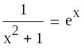
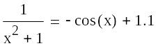
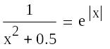
7. Solve the system of equations graphically
1. |
y
|
11. |
|
2. |
y y=x3–3x2+3x–9 |
12. |
y=sin(x2) |
3. |
y=sin(x2) |
13. |
|
4. |
y y+||x|–1|=0 |
14. |
y =sin(x2) y=||x|–1| |
5. |
y =e|x+2|
|
15. |
0=x3–3x2+3x–9–3y |
6. |
=1/3 |
16. |
cos()=0 |
7. |
/2= cos() |
17. |
cos() –=0 |
8. |
=5 |
18. |
cos(5) 4= |
9. |
2–cos2()=0 |
19. |
cos() |
10. |
=1/2 |
20. |
2 |
 =||x|–1|
 =|x2–9|
 =x3–3x2+3x–9
 cos(0.5)
 cos()
cos()
8. Solve equation numerically. Find all roots. Use graphs to know number of roots.
In report show zoomed area of graphs with roots.
1. |
|
11. |
|
2. |
ln(x)=–x |
12. |
|
3. |
ln(|x|)=–|x| |
13. |
|
4. |
|
14. |
|
5. |
|
15. |
|
6. |
|
16. |
|
7. |
|
17. |
|
8. |
|
18. |
|
9. |
|
19. |
|
10. |
|
20. |
|

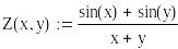
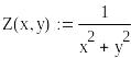
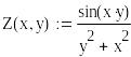
9. Build 3d surface. Use corresponding axes scale. Use colormap, lighting and choose the best view.
1 |
|
11 |
|
2 |
|
12 |
|
3 |
|
13 |
|
4 |
|
14 |
|
5 |
|
15 |
|
6 |
|
16 |
|
7 |
|
17 |
|
8 |
|
18 |
|
9 |
|
19 |
|
10 |
|
20 |
|
10. Create the animation using N as a number of the frame. Fix the scale of axes. Set framerate 25 frames per second. Total number of frames must be chosen for good viewing. In report show saved avi-file.
1. |
y1=sin(x+N/5) y2=3sin(x-N/5) y=y1+y2 |
11 |
( |
2. |
y=(5-N)x |
12 |
y=sin(N/x) |
3. |
cos(5+N/5) |
13 |
sin(6+N/5) |
4. |
y=N/x |
14 |
cos(3+N/6) |
5. |
|
15 |
|
6. |
( |
16 |
|
7. |
( |
17 |
( |
8. |
|
18 |
sin(+N/5) |
9. |
cos(4+N/5) |
19 |
sin(–N/5) |
10. |
sin(–N/6) |
20 |
y= sin(x+N/5)+ sin(x–N/5) |
 parametric
coordinates)
parametric
coordinates)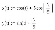 parametric
coordinates)
parametric
coordinates) parametric
coordinates)
parametric
coordinates)
11. Complete differential equation describing oscillation of the ball with mass m on the spring with rigidity k in viscid environment where resistance force is proportional to velocity as F = z·v. External force and initial conditions are given in the table as well as parameters m, k and z.
Variant N |
m |
k |
z |
x(0) |
v(0) |
F(t) |
1 |
1 |
1 |
0.1 |
3 |
0 |
5 sin(3t) |
2 |
1 |
0.2 |
0.1 |
3 |
0 |
5 sin(3t) |
3 |
1 |
1 |
0.1 |
0 |
0 |
5 sin(3t) |
4 |
4 |
1 |
0.5 |
1 |
0 |
10 sin(3t) |
5 |
10 |
0.4 |
3 |
0 |
5 |
0 |
6 |
10 |
4 |
1 |
0 |
5 |
0 |
7 |
2 |
4 |
1.5 |
0 |
0 |
sin(x)/|sin(x)| |
8 |
1 |
1 |
0.1 |
3 |
0 |
5·sin(t) |
9 |
1 |
1 |
0.01 |
3 |
0 |
5·sin(0.85·t) |
10 |
1 |
1 |
0.1 |
5 |
0 |
5·sin(0.1·t) |
11 |
2 |
2 |
0.01 |
5 |
0 |
5·sin(1.4·t) |
12 |
2 |
2 |
1 |
0 |
100 |
50·sin(2·t) |
13 |
2 |
10 |
0.5 |
3 |
0 |
5·sin(0.2·t) |
14 |
2 |
10 |
0.05 |
3 |
0 |
5·sin(0.2·t) |
15 |
2.5 |
9 |
0.05 |
0 |
10 |
15·sin(0.2·t) |
16 |
0.8 |
1 |
0.1 |
0 |
0 |
5 sin(2.8·t) |
17 |
10 |
4 |
1 |
5 |
0 |
0 |
18 |
1 |
1 |
0.1 |
3 |
4 |
5·sin(0.9t) |
19 |
1 |
1 |
0.02 |
4 |
0 |
5·sin(0.85·t) |
20 |
2 |
2.2 |
1 |
10 |
100 |
40·sin(2.2·t) |
12. Create the animation of ball oscillation corresponding solution of diff.equation from task 11. Draw the ball using parametric circle equation in x-y coordinate.
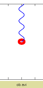 <–Click
it (Example)
<–Click
it (Example)
13. Build the mathematical model of ecological system “predator-prey”.
Let x0(t) is the number of some predator (for example, wolves);
x1(t) is the number of its prey (for example, rabbits);
then dx0(t)/dt and dx1(t)/dt are the speeds of the two populations changing;
The dynamics of the populations can be described by equations:
dx0 /dt = a·x0 – b x0 x1
dx1 /dt = – c·x1 + k x0 x1
The first equation can be interpreted as: the change in the prey's numbers is given by its own growth which is proportional to their numbers (a·x0), minus the rate at which it is preyed upon (b x0 x1). The preys are assumed to have an unlimited food supply.
The second equation expresses the change in the predator population as growth fueled by the food supply (k x0 x1, preys are food for predators), minus natural death (c·x1).
Variant N |
a |
b |
c |
k |
x0(0) |
x1(0) |
1 |
1 |
0.06 |
0.01 |
0.005 |
10 |
10 |
2 |
0.8 |
0.09 |
0.08 |
0.01 |
10 |
10 |
3 |
0.8 |
0.2 |
0.8 |
0.05 |
20 |
5 |
4 |
0.1 |
0.05 |
0.8 |
0.03 |
20 |
2 |
5 |
0.1 |
0.01 |
0.8 |
0.05 |
15 |
2 |
6 |
0.3 |
0.01 |
0.7 |
0.003 |
10 |
5 |
7 |
0.8 |
0.09 |
0.07 |
0.01 |
20 |
5 |
8 |
0.8 |
0.002 |
0.4 |
0.005 |
50 |
10 |
9 |
1.9 |
0.05 |
0.2 |
0.02 |
80 |
50 |
10 |
1.9 |
0.05 |
0.9 |
0.02 |
80 |
50 |
11 |
3 |
0.2 |
0.9 |
0.02 |
50 |
10 |
12 |
2 |
0.2 |
0.9 |
0.08 |
20 |
10 |
13 |
0.2 |
0.03 |
0.04 |
0.001 |
30 |
5 |
14 |
0.4 |
0.002 |
0.8 |
0.007 |
3 |
10 |
15 |
1 |
0.06 |
0.8 |
0.07 |
3 |
100 |
16 |
2.2 |
0.06 |
0.8 |
0.07 |
2 |
40 |
17 |
3 |
0.06 |
0.4 |
0.09 |
2 |
40 |
18 |
1 |
0.6 |
0.4 |
0.1 |
30 |
4 |
19 |
1.2 |
0.8 |
0.3 |
0.01 |
20 |
2 |
20 |
1.2 |
0.03 |
0.1 |
0.001 |
10 |
85 |
Draw the graphs of populations dynamics (x vs time) for time period = 100 (months). Also draw the graph x0 vs x1. Make the conclusion about the ecological system behavior.