Implications of Strict Exogeneity

The strict exogeneity assumption has several implications.

• The unconditional mean of the error term is zero, i.e.,

(1.1.8)

This is because, by the Law of Total Expectations from basic probability theory,²

• If the cross moment of two random variables and is zero, then we say that is orthogonal to (or is orthogonal to ). Under strict exogeneity, the regressors are orthogonal to the error term for all observations, i.e.,

or

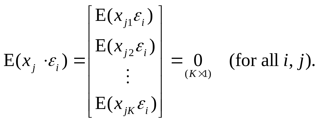(1.1.9)

The proof is a good illustration of the use of properties of conditional expecta­tions and goes as follows.

Proof. Since is an element of strict exogeneity implies

(1.1.10)

by the Law of Iterated Expectations from probability theory.³ It follows from this that

⁴)

The point here is that strict exogeneity requires the regressors be orthogonal not only to the error term from the same observation (i.e., for all ), but also to the error term from the other observations (i.e., for all and for ).

• Because the mean of the error term is zero, the orthogonality conditions (1.1.9) are equivalent to zero-correlation conditions. This is because

In particular, for Therefore, strict exogeneity implies the requirement (familiar to those who have studied econometrics before) that the regressors be contemporaneously uncorrelated with the error term.

Strict Exogeneity in Time-Series Models

For time-series models where is time, the implication (1.1.9) of strict exogeneity can be rephrased as: the regressors are orthogonal to the past, current, and future error terms (or equivalently, the error term is orthogonal to the past, current, and future regressors). But for most time-series models, this condition (and a fortiori strict exogeneity) is not satisfied, so the finite-sample theory based on strict exogeneity to be developed in this section is rarely applicable in time-series contexts. However, as will be shown in the next chapter, the estimator possesses good large-sample properties without strict exogeneity.

The clearest example of a failure of strict exogeneity is a model where the regressor includes the lagged dependent variable. Consider the simplest such model:

(1.1.11)

This is called the first-order autoregressive model (AR(1)). (We will study this model more fully in Chapter 6.) Suppose, consistent with the spirit of the strict exogeneity assumption, that the regressor for observation is orthogonal to the error term for so Then

Therefore, unless the error term is always zero, is not zero. But is the regressor for observation Thus, the regressor is not orthogonal to the past error term, which is a violation of strict exogeneity.

Other Assumptions of the Model

The remaining assumptions comprising the classical regression model are the

following.

Assumption 1.3 (no multicollinearity): The rank of the data matrix, is with probability 1.

Assumption 1.4 (spherical error variance):

⁵ (1.1.12)

(no correlation between observations)

(1.1.13)

To understand Assumption 1.3, recall from matrix algebra that the rank of a matrix equals the number of linearly independent columns of the matrix. The assumption says that none of the columns of the data matrix can be expressed as a linear combination of the other columns of .That is, is of full column rank. Since the columns cannot be linearly independent if their dimension is less than , the assumption implies that i.e., there must be at least as many observations as there are regressors. The regressors are said to be (perfectly) multicollinear if the assumption is not satisfied. It is easy to see in specific applications when the regressors are multicollinear and what problems arise.

Example 1.4 (continuation of Example 1.2): If no individuals in the sam­ple ever changed jobs, then for all in violation of the no multicollinearity assumption. There is evidently no way to distinguish the tenure effect on the wage rate from the experience effect. If we substitute this equality into the wage equation to eliminate the wage equation becomes

which shows that only the sum but not and separately, can be estimated.

The homoskedasticity assumption (1.1.12) says that the conditional second moment, which in general is a nonlinear function of is a constant. Thanks to strict exogeneity, this condition can be stated equivalently in more familiar terms. Consider the conditional variance It equals the same constant because

Similarly, (1.1.13) is equivalent to the requirement that

That is, in the joint distribution of conditional on the covariance is zero. In the context of time-series models, (1.1.13) states that there is no serial correla­tion in the error term.

Since the element of the matrix is Assumption 1.4 can be written compactly as

(1.1.14)

The discussion of the previous paragraph shows that the assumption can also be written as

However, (1.1.14) is the preferred expression, because the more convenient mea­sure of variability is second moments (such as ) rather than variances. This point will become clearer when we deal with the large sample theory in the next chapter. Assumption 1.4 is sometimes called the spherical error variance assumption because the matrix of second moments (which are also variances and covariances) is proportional to the identity matrix This assumption will be relaxed later in this chapter.

The Classical Regression Model for Random Samples

The sample is a random sample if is i.i.d. (independently and iden­tically distributed) across observations. Since by Assumption 1.1 is a function of and since is independent of for is inde­pendent of for So

(1.1.15)

(Proving the last equality in (1.1.15) is a review question.) Therefore, Assumptions 1.2 and 1.4 reduce to

(1.1.16)

(1.1.17)

The implication of the identical distribution aspect of a random sample is that the joint distribution of does not depend on So the unconditional second moment is constant across (this is referred to as unconditional homoske­dasticity) and the functional form of the conditional second moment is the same across However, Assumption 1.4 — that the value of the conditional second moment is the same across - does not follow. Therefore, Assumption 1.4 remains restrictive for the case of a random sample; without it, the conditional sec­ond moment can differ across through its possible dependence on To emphasize the distinction, the restrictions on the conditional second moments, (1.1.12) and (1.1.17), are referred to as conditional homoskedasticity.

“Fixed” Regressors

We have presented the classical linear regression model, treating the regressors as random. This is in contrast to the treatment in most textbooks, where is assumed to be “fixed” or deterministic. If is fixed, then there is no need to distinguish between the conditional distribution of the error term, , and the unconditional distribution, so that Assumptions 1.2 and 1.4 can be written as

(1.1.18)

(1.1.19)

Although it is clearly inappropriate for a nonexperimental science like economet­rics, the assumption of fixed regressors remains popular because the regression model with fixed can be interpreted as a set of statements conditional on allowing us to dispense with “ ” from the statements such as Assumptions 1.2 and 1.4 of the model.

However, the economy in the notation comes at a price. It is very easy to miss the point that the error term is being assumed to be uncorrelated with current, past, and future regressors. Also, the distinction between the unconditional and condi­tional homoskedasticity gets lost if the regressors are deterministic. Throughout this book, the regressors are treated as random, and, unless otherwise noted, state­ments conditional on are made explicit by inserting “ ”.

QUESTIONS FOR REVIEW

1. (Change in units in the semi-log form) In the wage equation, (1.1.3), of Exam­ple 1.2, if is measured in cents rather than in dollars, what difference does it make to the equation? Hint:

2. Prove the last equality in (1.1.15). Hint: is independent of for

3. (Combining linearity and strict exogeneity) Show that Assumptions 1.1 and 1.2 imply

(1.1.20)

Conversely, show that this assumption implies that there exist error terms that satisfy those two assumptions.

4. (Normally distributed random sample) Consider a random sample on con­sumption and disposable income, Suppose the joint distribution of (which is the same across because of the random sample assumption) is normal. Clearly, Assumption 1.3 is satis­fied; the rank of would be less than only by pure accident. Show that the other assumptions, Assumptions 1.1, 1.2, and 1.4, are satisfied. Hint: If two random variables, and are jointly normally distributed, then the conditional expectation is linear in i.e.,

and the conditional variance, does not depend on Here, the fact that the distribution is the same across is important; if the distribution differed across and could vary across

5. (Multicollinearity for the simple regression model) Show that Assumption 1. 3 for the simple regression model is that the nonconstant regressor is really nonconstant (i.e., for some pairs of with probability one).

6. (An exercise in conditional and unconditional expectations) Show that As­sumptions 1.2 and 1.4 imply

(*)

Hint: Strict exogeneity implies So (*) is equivalent to