3. Putting the is and the lm Relations Together

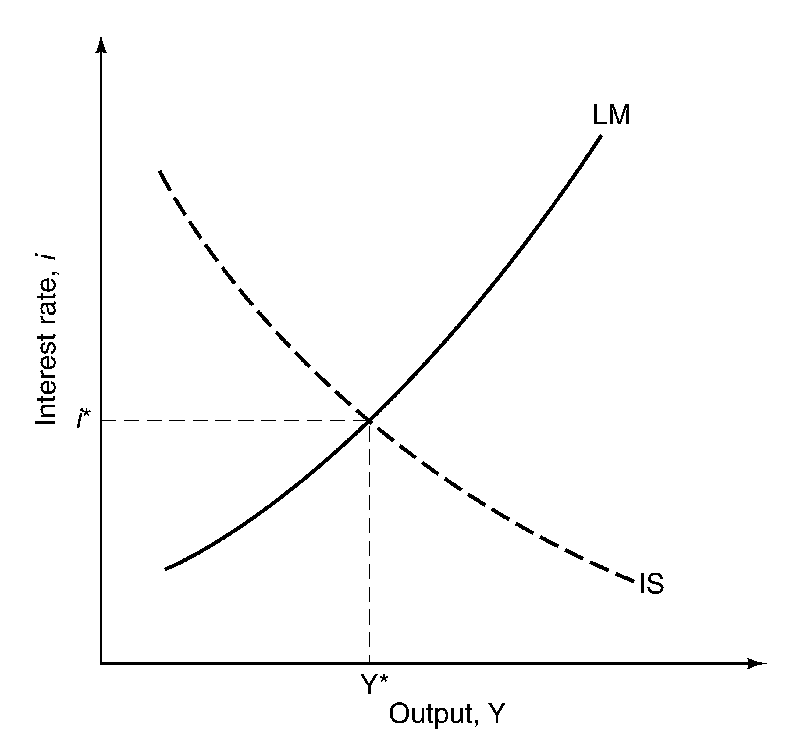
The equilibrium values of i and Y are those that satisfy simultaneously the goods market equilibrium condition (equation (5.2)) and the money market equilibrium condition (equation (5.3)). Graphically, these values are determined by the point of intersection of the IS and LM curves, as illustrated in Figure 5.1.

Changes in the equilibrium values of output and the interest rate (Y* and i*) can be brought about only as the result of shifts in the IS curve, the LM curve, or both. An increase in the money supply, which shifts the LM curve down, increases equilibrium output and reduces the equilibrium interest rate. An increase in taxes (or a reduction in government spending), which shifts the IS curve to the left, reduces equilibrium output and reduces the equilibrium interest rate. The text notes that an increase in taxes will have an ambiguous effect on investment, since the output effect tends to reduce investment, but the interest rate effect tends to increase it. More generally, although deficit reduction increases public (government) saving, it does not necessarily increase investment, because private saving is endogenous.

Figure 5.1: The IS-LM Model

4. Using a Policy Mix

The text considers the consequences of combinations of fiscal and monetary policy through two examples: the recession of 2001 and the deficit reduction during President Clinton’s first term. A box in the text argues that the proximate cause of the recession of 2001 was a drop in (nonresidential) investment spending and that the policy response – a sharp cut in interest rates by the Fed and large tax cuts spearheaded by the Bush administration – lessened the severity of the recession. Although the tax cuts provided useful stimulus, they also played the major role in creating large budget deficits in the United States. Many economists worry about these deficits, and argue that the tax cuts should not have been made permanent. The recession is over, but the loss of tax revenue continues to affect government finances.

During the recession of 2001, monetary and fiscal policy both became more expansionary. In the President Clinton’s first term, by contrast, fiscal policy became more contractionary while monetary policy became more expansionary. The Federal Reserve supported the Clinton deficit reduction policy (a fiscal contraction) with a monetary expansion, and interest rates fell. As a result, there was a deficit reduction without a slowdown in growth. In fact, there was a large economic expansion – an outcome supported by the policy mix but also aided by other factors.

5. How Does the is-lm Model Fit the Facts?

So far, the discussion has ignored dynamics. In fact, it takes some time for consumption, investment, and output to adjust to an economic disturbance. How long is an empirical question. To discuss this question and to provide evidence of the empirical relevance of the IS-LM model, the text describes the results presented in Christiano, Eichenbaum, and Evans, “The Effects of Monetary Policy Shocks: Evidence From the Flow of Funds,” Review of Economics and Statistics, February 1996. The paper describes the dynamic responses of several important macroeconomic variables to an increase in the federal funds rate, i.e., a monetary contraction. An interest rate increase does lead to a decline in output, as the IS-LM model would predict, but adjustment happens relatively slowly. It takes almost two years for monetary policy to have its full effect on output. The price level remains more or less unchanged for about six quarters and then declines. Thus, the fixed-price assumption may be reasonable for the short run.