Ranking and sorting data I

April 25th, 2005

Computing the rank order of entries in an array of data is needed in many applications.

There are a number of builtin OOo functions that deal with the ranking and ordering of data. We will look at four - RANK, PERCENTRANK, PERCENTILE, and LARGE

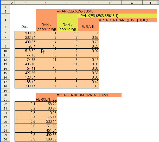
In the example below, we see two variants of RANK wherein the entries can be ordered in descening or ascending order. The first two arguments of RANK are the value to be ranked and the array that contains the data. By default, with these two arguments, the entries will be ranked in descending order. The optional third argument - when set to 1 - ranks the entires in ascending order.

The PERCENTRANK function assigns a percentage value to a given value based on a 100% range between the minumum and maximum values of the specified range. If you don’t format these results as a percentage value, the output from PERCENTRANK will lie betwen 0 and 1.

The PERCENTILE function accepts a percentage value as input and returns the percentile of data values in an array. A percentile returns the scale value for the array which goes from the smallest (%age=0) to the largest value (%age=1) of the array. The 50% percentile of an array is the same as the MEAN.

Posted in Function Tips | 1 Comment »

Conditional summation revisited

April 20th, 2005

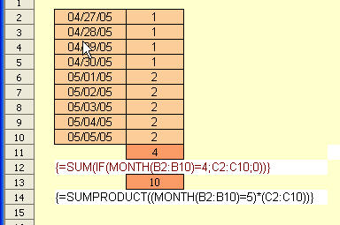
For OOo 2.0, enhanced functionality seems to have been introduced with respect to using array formulas for conditional summation. Consider the example below, where we wish to total numbers in a column corresponding to a particular month.

Contrast this with the use of SUMIF in a previous tip. We have also covered SUMPRODUCT before

Now, the SUM IF and SUMPRODUCT constructs shown below accept a function of an array. MONTH normally accepts a single date as a parameter - but within an array formula as in the examples below, it makes more sense to be able to apply an array of dates to MONTH. This has always been possible in Excel.

It seems, OOo Calc continues to match and/or surpass Excel in functionality - which can onloy be a good thing for those who wish to migrate from Excel.

Posted in Function Tips | No Comments »

Regression analysis I : Basic linear formulas

April 12th, 2005

As requested by Joerg in Germany, I am going to cover the topic of regression analysis over the next few days - including formulas, built-in functions and charting with trendlines.

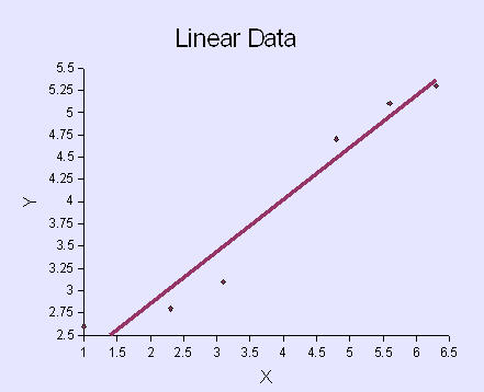
Consider a set of data point pairs - which suggests a possible linear relationship between the two variables.

The equations below are used to calculate the slope m and y-intercept point b for a given set of data, as well as the correlation coefficient r.

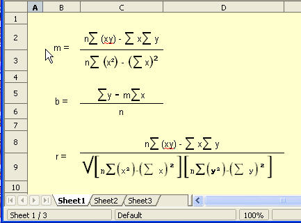
Given the formula above, it is a straightforward process to extract the linear coefficients for the given set of data points.

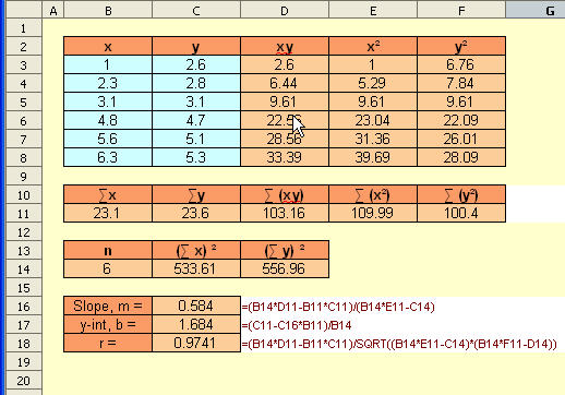
Next, we will look at buil-in OOo Calc functions and the plotting of the trendline for this linear regression example.

Posted in Math & Statistics | No Comments »

Regression Analysis II : Basic functions, charting

April 13th, 2005

n a continuation from the previous tip, we look at some basic built-in functions for determining trendline coefficients of a X-Y plot.

For a series of X-Y values that we suspect have a linear relationship, we can determine the slope and y-intercept values of the linear approximation using the builtin functions SLOPE() and INTERCEPT as showb below. Compare these values to those we obtained when performig our regression analysis without using the builtin functions.

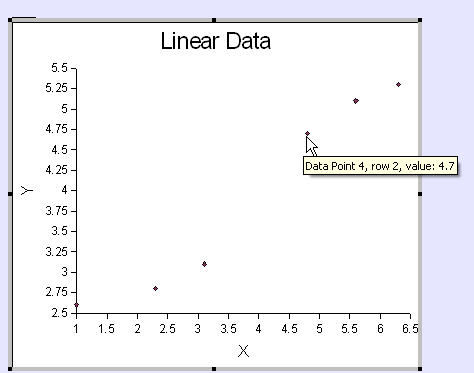
Now, plotting X-Y data is straightforward. Adding a trendline takes a little more work. We start off with the basic X-Y plot.

First, select the chart for editing by right-clicking anywhere inside the chart boundary. Now, before we add the trendline, we need to select the data series for editing. Move the cursor over one of the data points - you will see popup info about the nearest data point.

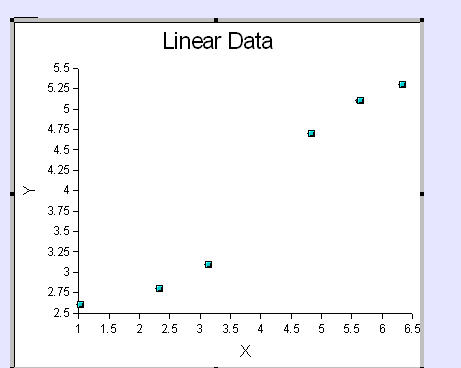
Left-click and the data series is now selected (below)

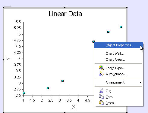
Now right-click and select Object Properties (below)

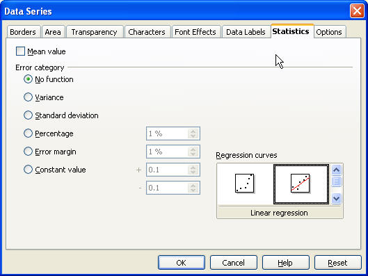
The Data Series dialog opens up. Select the Statistics tab (below). Select the Linear Regression curve and click OK

The modified X-Y plot with the newly added trend line.

Posted in Math & Statistics | 1 Comment »