Charting: Editing charts : part 2

In this tip, we see how to modify the attributes of the axes on an already created chart.

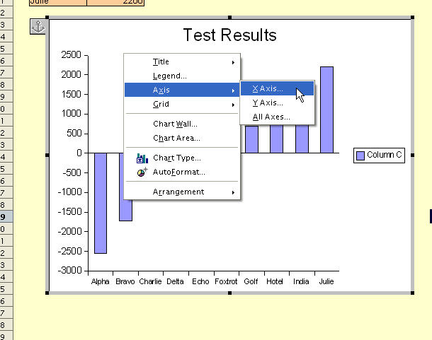
before you can modify the appearance of the x-axis of the chart, you need to make sure the chart is selected for editing ( a solid green border) Within the boundaries of the chart, select Axis - X-Axis as shown below. This opens the X-Axis dialog.

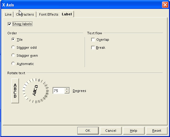
There are a number of available tabs. We wish to rotate the text on the axis, so we choose the Label tab.

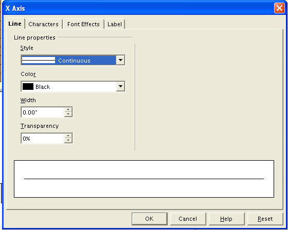
Another useful tab is the Line tab, but we will not change any of the default properties here.

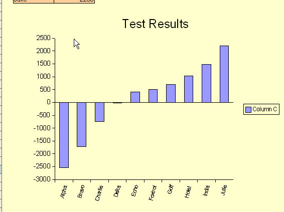
The final result (for now) I suggest that you experiment with all the available dialogs and tabs to become familar with the powerful chart editing capabilities offered by OOo Calc.

This entry was posted on Monday, D

Charting: Editing charts : part 3

In this short tutorial, we will change the attributes of the chart title and the chart legend.

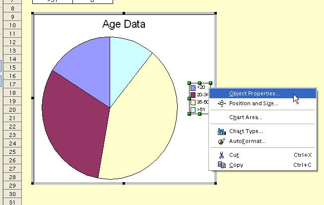
First, select the chart and go into Edit mode. Select the Legend object and click on Object properties as shown below.

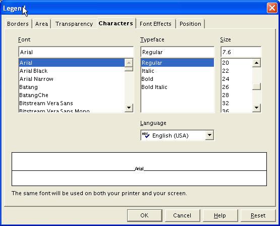
In the Object Proiperties dialog, select the Characters tab. We will increase the font size a few points.

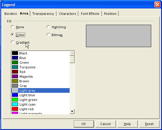
In the Area tab, we will add some grey background fill.

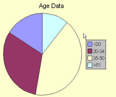
With the desired modifications complete, click OK to close the dialog. The modified chart is shown below.

This entry was posted on Saturda

Autocorrect

When entering text in OO Calc cells, you may notice that the program makes assumptions about what you are typing and you get unwanted corrections.

These corrections are completely configurable throught theAutoCorrect dialog.

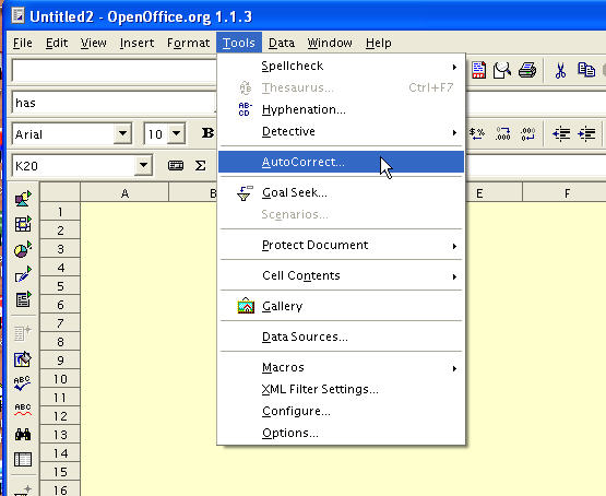
The AutoCorrect dialog is invoked by selecting Tools - AutoCorrect as shown below.

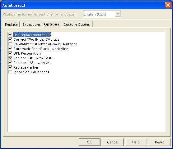
The Options tab presents some optional corrections that OOo Calc can perform on any text entered by the user. From the identifier of each option, it should be easy to understand what OOo Calc plans to do - if that option is enabled.

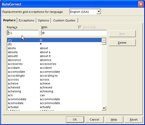
In particular, the user can make use of a replacement table of common mispellings. The replacement table is fully configurable via the Replace tab - shown below.For example, if “acn” is a string you use often (a name of a company perhaps) OOo Calc will always insist on replacing it with “can”. By removing this particular entry from the replacement table, OOo Calc will leave “acn” alone.

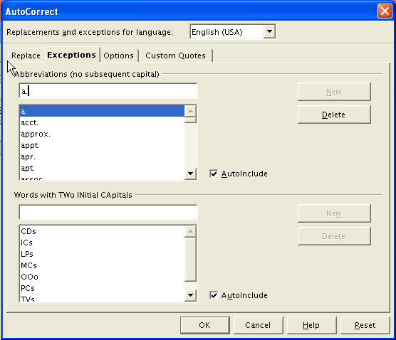
The Exceptions tab - see below - allows the user to prevent OOo Calc from correcting certain 2-letter initial cap combinations.

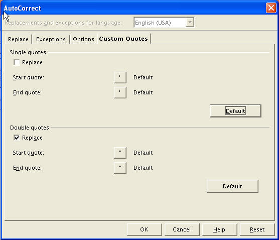
Finally, the Custom Quotes tab allows the user to replace single/double quotation marks with any characters of his/her choosing.

This entry was posted on Friday, November 26th, 2004 at 9:07 pm and is filed underUsing OpenOffice Calc. You can follo

Macros: Getting Cell Information

Invariably, macros written for use within the Calc application will need to access the contents of the cells on a spreadsheet. This tip is an introduction to the various available methods.

The three methods we will look at are getCellByPosition,getCellRangeByPosition and getCellRangeByName

The function that is first encountered for most people isgetCellByPosition. In the sample below, we access cell A1 (on Sheet1)

Sub getCellInfo ‘get the first sheet of the spreadsheet doc xSheet = ThisComponent.Sheets(0)

‘Get value of Cell A1 A1_value = xSheet.getCellByPosition(0,0).value

print A1_value

End Sub

The second example shows the use of getCellRangeByName and may be easier to use - because the cells are referenced by the traditional column/row identifiers that are displayed along each axis. However, for applications requiring looping through an array of cells, getCellByPosition is easier to use.

Sub getCellInfo ‘get the first sheet of the spreadsheet doc xSheet = ThisComponent.Sheets(0)

‘Get value of Cell A3 A3_value = xSheet.getCellRangeByName(”A3″).value

print A3_value

End Sub

The next example shows how getCellInfo grabs an array of cells -myTable. A subsequent call to getCellByPosition for themyTable object is relative to the origin of this array.

Sub getCellInfoByRange Dim myTable as Object

‘get the first sheet of the spreadsheet doc xSheet = ThisComponent.Sheets(0)

‘Grab array A3:A5 myTable = xSheet.getCellRangeByName(”A3:A5″) A5_value = myTable.getCellByPosition(0,2).value

print A5_value

End Sub

The final method that needs discussion isgetCellRangeByPosition and the example below illustrates it’s use. It is equivalent in functionality to the previous example.

Sub getCellInfoByRange Dim myTable as Object

‘get the first sheet of the spreadsheet doc

xSheet = ThisComponent.Sheets(0)

‘Grab array A3:A5 myTable = xSheet.getCellRangeByPosition(0,2,0,4) A5_value = myTable.getCellByPosition(0,2).value print A5_value

End Sub