Basic functions : sumif

This short tutorial illustrates the two basic ways that SUMIF can be used in a spreadsheet.

The SUMIF function takes two or three arguments.

For the two argument version, the condition is applied to each cell in the range being SUMmed. In the example below, C9 is the sum of all values in C3:C8 that are greater than 5.

In the three argument version, the condition is applied to a separate range of cells. This range can be numerical of textual. In the example below, the values corresponding to Tom are summed in C10

This entry was posted on Thursday, December 9th, 2004 at 10:34 pm and is filed underFunction Tips. You can follow an

Adding a background graphic

For a more visually presentable spreadsheet, it is possible to add a background image. Here is a quick tutorial on adding an image to the background.

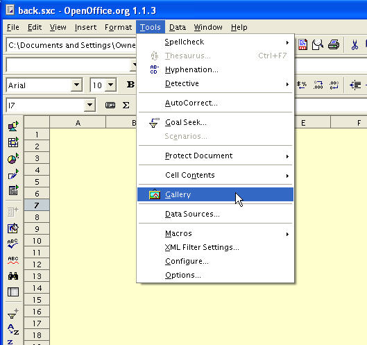
We first activate the built in gallery of images, icons & backgrounds by selecting Tools - Gallery

Select the Backgrounds option and drag the desired background onto the spreadsheet.

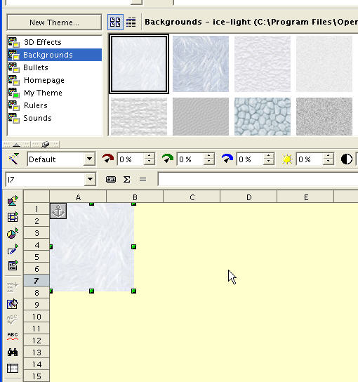
The selected image is active when placed. Adjust it’s position and size so that it fills the spreadsheet. Then select Arrange - To Background as shown below.

We are done. If you have alternative technique for placing graphic backgounds on spreadsheets, I’d like to hear from you.

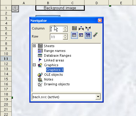
Update: To bring the background image to the foreground again, the following steps need to be performed.

Open the Navigator as shown below.

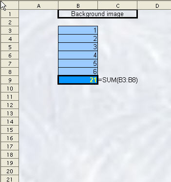
Under Graphics, select the required image - in our example, there is only one. The anchor symbol should appear as shown below.

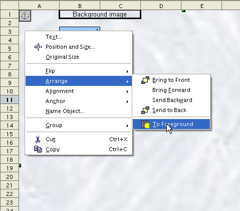
To bring the now selected graphic to the foreground, selectArrange - To Foreground by right-clicking on a empty part of the background as shown below.

This entry was posted on Tue

« Adding a background graphic

Introduction to the Status Bar » Using the Navigator

The Navigator, as the name suggests, allows you to view the contents of a spreadsheet, sheets, ranges, linked areas, graphics objects, and notes.

For simple, single page spreadsheets, the use of the Navigatormight be overkill, but as the complexity of the spreadsheet document increases, it can quickly prove it’s usefulness.

There are three ways to invoke the Navigator

Firstly, there is an icon on the toolbar as shown below.

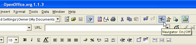
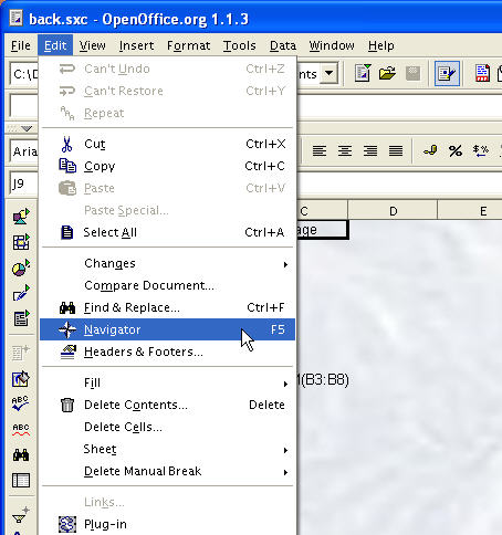
You can also select Edit - Navigator. Also, by default, the function key F5 will toggle the Navigator window ON/OFF

The Navigator window is shown below. It identifies all objects in the document and allows the user to select any object for further manipulation. For example. background images can only be selected through the Navigator

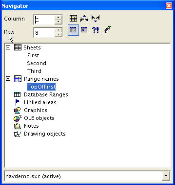
In the example below, we double-click on the named range and it is selected and highlighted for us.

This entry was posted on Monday, Jan

Introduction to the Status Bar

How many of us have paid any attention to the row of small windows at the bottom of the OpenOffice Calc window? In this article, we will explore the Status Bar in more depth.

The Status Bar displays information about the current sheet. It is shown below in the default configuration with the different fields tagged.

The fields in the default configuration are:

• 1 : Position The number of the current sheet and the total number of sheets in the document.

• 2 : Page Style The Page Style of the currently open sheet. You can double-click in this field to call up the Page Style Editor.

• 3 : Zoom The current page display zoom factor.

• 4 : Insert Mode The current insert mode. This field is active when the cursor is in the input line of a formula or cell. By clicking in this field, you can toggle between INSRT = insert and OVER = overwrite.

• 5 : Selection Mode The current selection mode. By clicking in this field, you can toggle between STD = Standard (default), EXT = Extend and ADD = Add.

• 6 : Modified Flag If modifications to the current document have not been saved, a * is displayed here.

• 7 : Formula A basic evaluation of a simple formula for the currently selected range is displayed here. Default is SUM

The Status Bar can be customized by clicking Tools - Configureand selecting the Status Bar tab. The Status Bar configurtion dialog window is shown below.

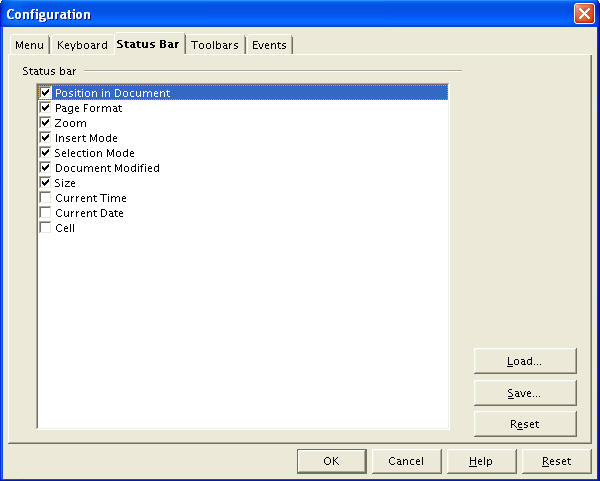
Th

is entry was posted on We