Rounding Numbers to Thousands and Millions

February 12th, 2005

Often, in financial statements, we wish to express totals as ‘Thousands’ or ‘Millions’. In Calc, we use custom formatting to do this.

In the example below, we use the number 1234567 to illustrate how the custom formats affect how this is displayed.

Firstly, #,## controls the use of commas. Secondly, 0 controls the number of digits after the decimal point. Finally, the trailing commas control the rounding of the number to thousands and millions.

Posted in Finance | No Comments »

Text manipulation 1 : Concatenation

February 6th, 2005

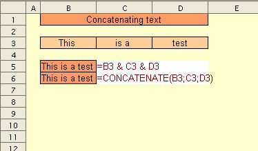
There are two methods available for concatenating text.

The ampersand symol & can be used as a concatenation operator on text - as shown below. This is analogous to the + operator for numbers.

There is also a CONCATENATE function - which can be used on up to 30 strings. The CONCATENATE function is also shown in the example below.

Copying Formulas while preserving references

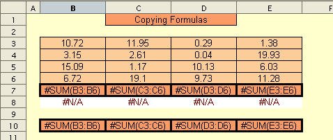
When you cut and paste formulas from a range of cells, the cell references within the formulas will be automatically adjusted. Here, we show how to work aroud this ‘feature’.

For the purposes of illustration - we consider the simple example below - with the four formulae in B7:E7

WIth B7:E7 selected, we select Edit - Find & Replace We will be replacing the “=” characters with “#” in each formula. Now, we have a range of text values that will be unchanged in a cut/paste or copy/pastee operation.

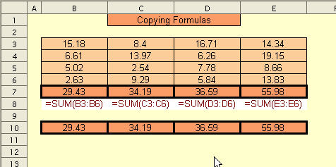
We can now copy/paste on the range of text values.

The last step is to use Find & Replace to restore the original formulae by replacing “#” with “=”, reversing the previous Find & Replace operation.

This entry was posted on Friday, January 28th, 2005 at 9:47 pm and is filed under Using OpenOffice Calc. You can follow any responses to this entry thro

Sumproduct and conditional summation

January 20th, 2005

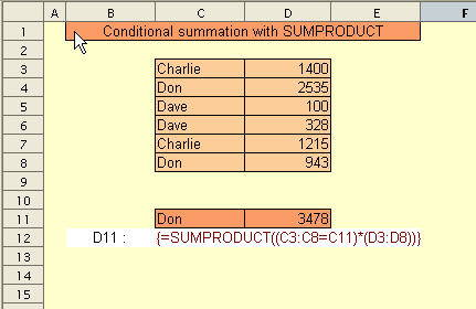
In this tip, we see how powerful SUMPRODUCT as an array function can be when doing condition summations.

In the example below, we wish to sum up any numbers in column D that correspond to the person referenced in C11. Whenever the value of the data in C3:C8 matches C11, the corresponding number inD3:D8 is added to the total.

D11 is an array formula, which is applied with CTRL - Shift - Enter

Posted 

Custom Time Formatting for a timesheet

January 16th, 2005

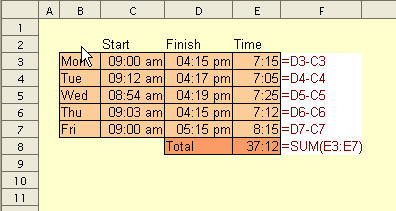
In the timesheet example below, to represent the total hours worked for the week, we use a custom time format [H]:MM

Cells E3:E7 are also formatted similarly. If we had used HH:MM, E3 for example would display 07:15 - which is not quite what we are looking for.

Cells C3:D7 are formatted HH:MM AM/PM

Posted i

Data Validation 101

The Data Validation feature of OOo Calc is similar to that in Excel. It helps the user control the data that is entered in the spreadsheet where it may be necessary to do so.

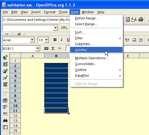
With a cell or range of cells selected, the Data Validation dialog can be activated with Data - Validity as shown below.

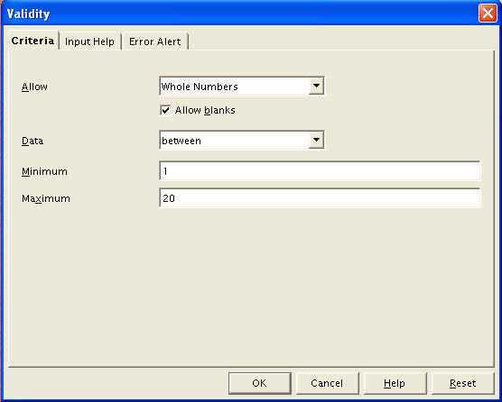
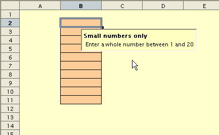
The Criteria tab allows you to define what type of data can be entered in the selected cells. In this example, we will restrict the data to whole numbers between 1 and 20.

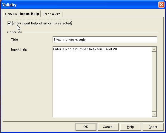
The Input Help tab allows the user to define a message box that appears when the cell is selected.

The Error Alert tab allows the user to define what happens when incorrect data is entered.

Here, we see the Input Help message when the user selects one of the cells of our range.

Here, we see the consequences of ignoring the help message.

This entry was posted on Tuesday, Ja