


Chapter
1 Complex ecological data sets
1.0 Numerical analysis of ecological data
The foundation of a general methodology for analysing ecological data may be derived from the relationships that exist between the conditions surrounding ecological observations and their outcomes. In the physical sciences for example, there often are cause-to-effect relationships between the natural or experimental conditions and the outcomes of observations or experiments. This is to say that, given a certain set of conditions, the outcome may be exactly predicted. Such totally deterministic relationships are only characteristic of extremely simple ecological situations.
|
Generally in ecology, a number of different outcomes may follow from a given set |
|
of conditions because of the large number of influencing variables, of which many are |
|
not readily available to the observer. The inherent genetic variability of biological |
|
material is an important source of ecological variability. If the observations are |
|
repeated many times under similar conditions, the relative frequencies of the possible |
Probability |
outcomes tend to stabilize at given values, called the probabilities of the outcomes. |
|
Following Cramér (1946: 148) it is possible to state that “whenever we say that the |
|
probability of an event with respect to an experiment [or an observation] is equal to P, |
|
the concrete meaning of this assertion will thus simply be the following: in a long |
|
series of repetitions of the experiment [or observation], it is practically certain that the |
|
[relative] frequency of the event will be approximately equal to P.” This corresponds to |
|
the frequency theory of probability — excluding the Bayesian or likelihood approach. |
|
In the first paragraph, the outcomes were recurring at the individual level whereas |
|
in the second, results were repetitive in terms of their probabilities. When each of |
Probability |
several possible outcomes occurs with a given characteristic probability, the set of |
distribution |
these probabilities is called a probability distribution. Assuming that the numerical |
Random |
value of each outcome Ei is yi with corresponding probability pi, a random variable (or |
variate) y is defined as that quantity which takes on the value yi with probability pi at |
|
variable |
each trial (e.g. Morrison, 1990). Fig. 1.1 summarizes these basic ideas. |
2 |
Complex ecological data sets |
|
|
|
O |
|
|
|
|
|
|
Case 1 |
B |
|
|
|
One possible outcome |
||
|
|
|
|||||
|
S |
|
|
|
|
|
|
|
E |
|
|
|
|
|
|
|
|
|
|
|
|
|
|
|
R |
|
|
|
|
|
|
|
V |
|
|
|
|
|
|
|
|
|
|
Outcome 1 |
|
Probability 1 |
|
|
A |
|
|
|
|
||
|
|
|
|
Outcome 2 |
|
Probability 2 |
|
Case 2 |
T |
|
|
|
. |
|
. |
|
|
|
. |
|
. |
||
|
|
|
|
|
|||
|
I |
|
|
|
|
||
|
|
|
|
. |
|
. |
|
|
O |
|
|
|
Outcome q |
|
Probability q |
|
N |
|
|
|
|
|
|
|
|
|
|
Random |
|
Probability |
|
|
S |
|
|
|
|
||
|
|
|
|
variable |
|
distribution |
|
|
|
|
|
|
|
||
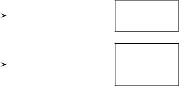
Figure 1.1 Two types of recurrence of the observations.
Events recurring at the individual level
Events recurring according to their probabilities
Of course, one can imagine other results to observations. For example, there may be strategic relationships between surrounding conditions and resulting events. This is the case when some action — or its expectation — triggers or modifies the reaction. Such strategic-type relationships, which are the object of game theory, may possibly explain ecological phenomena such as species succession or evolution (Margalef, 1968). Should this be the case, this type of relationship might become central to ecological research. Another possible outcome is that observations be unpredictable. Such data may be studied within the framework of chaos theory, which explains how natural phenomena that are apparently completely stochastic sometimes result from deterministic relationships. Chaos is increasingly used in theoretical ecology. For example, Stone (1993) discusses possible applications of chaos theory to simple ecological models dealing with population growth and the annual phytoplankton bloom. Interested readers should refer to an introductory book on chaos theory, for example Gleick (1987).
Methods of numerical analysis are determined by the four types of relationships that may be encountered between surrounding conditions and the outcome of observations (Table 1.1). The present text deals only with methods for analysing random variables, which is the type ecologists most frequently encounter.
The numerical analysis of ecological data makes use of mathematical tools developed in many different disciplines. A formal presentation must rely on a unified approach. For ecologists, the most suitable and natural language — as will become evident in Chapter 2 — is that of matrix algebra. This approach is best adapted to the processing of data by computers; it is also simple, and it efficiently carries information, with the additional advantage of being familiar to many ecologists.

Numerical analysis of ecological data |
3 |
|
|
Other disciplines provide ecologists with powerful tools that are well adapted to the complexity of ecological data. From mathematical physics comes dimensional analysis (Chapter 3), which provides simple and elegant solutions to some difficult ecological problems. Measuring the association among quantitative, semiquantitative or qualitative variables is based on parametric and nonparametric statistical methods and on information theory (Chapters 4, 5 and 6, respectively).
These approaches all contribute to the analysis of complex ecological data sets (Fig. 1.2). Because such data usually come in the form of highly interrelated variables, the capabilities of elementary statistical methods are generally exceeded. While elementary methods are the subject of a number of excellent texts, the present manual focuses on the more advanced methods, upon which ecologists must rely in order to understand these interrelationships.
In ecological spreadsheets, data are typically organized in rows corresponding to sampling sites or times, and columns representing the variables; these may describe the biological communities (species presence, abundance, or biomass, for instance) or the physical environment. Because many variables are needed to describe communities and environment, ecological data sets are said to be, for the most part, multidimensional (or multivariate). Multidimensional data, i.e. data made of several variables, structure what is known in geometry as a hyperspace, which is a space with many dimensions. One now classical example of ecological hyperspace is the fundamental niche of Hutchinson (1957, 1965). According to Hutchinson, the environmental variables that are critical for a species to exist may be thought of as orthogonal axes, one for each factor, of a multidimensional space. On each axis, there are limiting conditions within which the species can exist indefinitely; we will call upon this concept again in Chapter 7, when discussing unimodal species distributions and their consequences on the choice of resemblance coefficients. In Hutchinson’s theory, the set of these limiting conditions defines a hypervolume called the species’
Table 1.1 |
Numerical analysis of ecological data. |
|
|
|
|
|
Relationships between the natural conditions |
Methods for analysing |
|
and the outcome of an observation |
and modelling the data |
|
|
|
|
Deterministic: Only one possible result |
Deterministic models |
|
Random: Many possible results, each one with |
Methods described in this |
|
a recurrent frequency |
book (Figure 1.2) |
|
Strategic: Results depend on the respective |
Game theory |
|
strategies of the organisms and of their environment |
|
|
Uncertain: Many possible, unpredictable results |
Chaos theory |
|
|
|
4 |
|
|
Complex ecological data sets |
|||
|
|
|
|
|
|
|
|
|
|
|
|
|
|
|
From |
|
From |
|
From parametric and nonparametric |
|
|
mathematical algebra |
|
mathematical physics |
|
statistics, and information theory |
|
|
|
|
|
|
|
|
|
Matrix |
|
Dimensional |
|
Association among variables |
|
|
algebra (Chap. 2) |
|
analysis (Chap. 3) |
|
(Chaps. 4, 5 and 6) |
|
|
|
|
|
|
|
|
Complex ecological data sets
|
|
|
|
|
|
|
|
|
|
|
|
|
|
|
|
|
|
|
|
|
Ecological structures |
|
|
Spatio-temporal structures |
|
||||||||||
|
|
|
|
|
|
|
|
|
|
|
|
|
|
|
|
|
|
|
|
|
|
|
|
|
|
|
|
|
|
|
|
|
|
|
|
|
|
|
|
|
|
|
|
|
|
|
|
|
|
|
|
|
|
|
|
|
Association coefficients |
|
|
Time series |
|
|
|
Spatial data |
|
||||||
|
|
|
|
(Chap. 7) |
|
|
(Chap. 12) |
|
|
|
(Chap. 13) |
|
|||||
|
|
|
|
|
|
|
|
|
|
|
|
|
|
|
|
|
|
|
|
Clustering |
|
|
Ordination |
|
|
|
|
|
|
|
|
|
|
||
|
|
(Chap. 8) |
|
|
(Chap. 9) |
|
|
|
|
|
|
|
|
|
|
||
|
|
Agglomeration, |
|
Principal component and |
|
|
|
|
|
|
|
|
|
|
|||
|
|
division, |
|
correspondence analysis, |
|
|
|
|
|
|
|
|
|
|
|||
|
|
partition |
|
metric/nonmetric scaling |
|
|
|
|
|
|
|
|
|
|
|||
|
|
|
|
|
|
|
|
|
|
|
|
|
|
|
|
|
|
|
|
|
Interpretation of |
|
|
|
|
|
|
|
|
|
|
||||
|
|
ecological structures (Chaps. 10 and 11) |
|
|
|
|
|
|
|
|
|
|
|||||
|
|
|
|
|
|
|
|
|
|
|
|
|
|
|
|||
|
|
|
Regression, path analysis, |
|
|
|
|
|
|
|
|
|
|
||||
|
|
|
canonical analysis |
|
|
|
|
|
|
|
|
|
|
||||
|
|
|
|
|
|
|
|
|
|
|
|
|
|
|
|
|
|
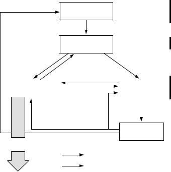
Figure 1.2 |
Numerical analysis of complex ecological data sets. |
|
|
|
|
|
|
|
|
||||||||
Fundamental |
fundamental niche. The spatial axes, on the other hand, describe the geographical |
||||||||||||||||
niche |
distribution of the species. |
|
|
|
|
|
|
|
|
||||||||
|
|
The quality of the analysis and subsequent interpretation of complex ecological |
|||||||||||||||
|
data sets depends, in particular, on the compatibility between data and numerical |
||||||||||||||||
|
methods. It is important to take into account the requirements of the numerical |
||||||||||||||||
|
techniques when planning the sampling programme, because it is obviously useless to |
||||||||||||||||
|
collect quantitative data that are inappropriate to the intended numerical analyses. |
||||||||||||||||
|
Experience shows that, too often, poorly planned collection of costly ecological data, |
||||||||||||||||
|
for “survey” purposes, generates large amounts of unusable data (Fig. 1.3). |
||||||||||||||||
|
|
The search for ecological structures in multidimensional data sets is always based |
|||||||||||||||
|
on association matrices, of which a number of variants exist, each one leading to |
||||||||||||||||
|
slightly or widely |
different results (Chapter |
7); even in |
so-called association-free |
|||||||||||||
Numerical analysis of ecological data |
5 |
|
|
New hypotheses |
General |
research area
Specific problem
WHAT: |
|
|
|
|
|
|
Sampling and |
|
|
|
|
||
Choice of variables |
|
|
|
Data analysis |
||
|
|
|||||
HOW: |
|
laboratory work |
|
|
||
|
|
|
|
|
||
Sampling design |
|
|
|
|
|
|
|
|
|
|
|
||
|
|
|
|
|
|
|
|
|
|
|
|
|
|
Conclusions
Unusable
data
Conjoncture Research objectives Previous studies Intuition
Literature Conceptual model
Descriptive statistics Tests of hypotheses Multivariate analysis Modelling
Research process
Feedback
Figure 1.3 Interrelationships between the various phases of an ecological research.
methods, like principal component or correspondence analysis, or k-means clustering, there is always an implicit resemblance measure hidden in the method. Two main avenues are open to ecologists: (1) ecological clustering using agglomerative, divisive or partitioning algorithms (Chapter 8), and (2) ordination in a space with a reduced number of dimensions, using principal component or coordinate analysis, nonmetric multidimensional scaling, or correspondence analysis (Chapter 9). The interpretation of ecological structures, derived from clustering and/or ordination, may be conducted in either a direct or an indirect manner, as will be seen in Chapters 10 and 11, depending on the nature of the problem and on the additional information available.
Besides multidimensional data, ecologists may also be interested in temporal or spatial process data, sampled along temporal or spatial axes in order to identify timeor space-related processes (Chapters 12 and 13, respectively) driven by physics or biology. Time or space sampling requires intensive field work, which may often be automated nowadays using equipment that allows the automatic recording of ecological variables, or the quick surveying or automatic recording of the geographic positions of observations. The analysis of satellite images or information collected by airborne or shipborne equipment falls in this category. In physical or ecological

Complex ecological data sets
applications, a process is a phenomenon or a set of phenomena organized along time or in space. Mathematically speaking, such ecological data represent one of the possible realizations of a random process, also called a stochastic process.
Two major approaches may be used for inference about the population parameters of such processes (Särndal, 1978; Koch & Gillings, 1983; de Gruijter & ter Braak, 1990). In the design-based approach, one is interested only in the sampled population and assumes that a fixed value of the variable exists at each location in space, or point in time. A “representative” subset of the space or time units is selected and observed during sampling (for 8 different meanings of the expression “representative sampling”, see Kruskal & Mosteller, 1988). Design-based (or randomization-based; Kempthorne, 1952) inference results from statistical analyses whose only assumption is the random selection of observations; this requires that the target population (i.e. that for which conclusions are sought) be the same as the sampled population. The probabilistic interpretation of this type of inference (e.g. confidence intervals of parameters) refers to repeated selection of observations from the same finite population, using the same sampling design. The classical (Fisherian) methods for estimating the confidence intervals of parameters, for variables observed over a given surface or time stretch, are
Model-based fully applicable in the design-based approach. In the model-based (or superpopulation) approach, the assumption is that the target population is much larger than the sampled population. So, the value associated with each location, or point in time, is not fixed but random, since the geographic surface (or time stretch) available for sampling (i.e. the statistical population) is seen as one representation of the superpopulation of such surfaces or time stretches — all resulting from the same generating process — about which conclusions are to be drawn. Under this model, even if the whole sampled population could be observed, uncertainty would still remain about the model parameters. So, the confidence intervals of parameters estimated over a single surface or time stretch are obviously too small to account for the among-surface variability, and some kind of correction must be made when estimating these intervals. The type of variability of the superpopulation of surfaces or time stretches may be estimated by studying the spatial or temporal autocorrelation of the available data (i.e. over the statistical population). This subject is discussed at some length in Section 1.1. Ecological survey data can often be analysed under either model, depending on the emphasis of the study or the type of conclusions one wishes to derive from them.
In some instances in time series analysis, the sampling design must meet the requirements of the numerical method, because some methods are restricted to data series meeting some specific conditions, such as equal spacing of observations. Inadequate planning of the sampling may render the data series useless for numerical treatment with these particular methods. There are several methods for analysing ecological series. Regression, moving averages, and the variate difference method are designed for identifying and extracting general trends from time series. Correlogram, periodogram, and spectral analysis identify rhythms (characteristic periods) in series. Other methods can detect discontinuities in univariate or multivariate series. Variation in a series may be correlated with variation in other variables measured
Numerical analysis of ecological data |
7 |
|
|
simultaneously. Finally, one may want to develop forecasting models using the Box & Jenkins approach.
Similarly, methods are available to meet various objectives when analysing spatial structures. Structure functions such as variograms and correlograms, as well as point pattern analysis, may be used to confirm the presence of a statistically significant spatial structure and to describe its general features. A variety of interpolation methods are used for mapping univariate data, whereas multivariate data can be mapped using methods derived from ordination or cluster analysis. Finally, models may be developed that include spatial structures among their explanatory variables.
For ecologists, numerical analysis of data is not a goal in itself. However, a study which is based on quantitative information must take data processing into account at all phases of the work, from conception to conclusion, including the planning and execution of sampling, the analysis of data proper, and the interpretation of results. Sampling, including laboratory analyses, is generally the most tedious and expensive part of ecological research, and it is therefore important that it be optimized in order to reduce to a minimum the collection of useless information. Assuming appropriate sampling and laboratory procedures, the conclusions to be drawn now depend on the results of the numerical analyses. It is, therefore, important to make sure in advance that sampling and numerical techniques are compatible. It follows that mathematical processing is at the heart of a research; the quality of the results cannot exceed the quality of the numerical analyses conducted on the data (Fig. 1.3).
Of course, the quality of ecological research is not a sole function of the expertise with which quantitative work is conducted. It depends to a large extent on creativity, which calls upon imagination and intuition to formulate hypotheses and theories. It is, however, advantageous for the researcher’s creative abilities to be grounded into solid empirical work (i.e. work involving field data), because little progress may result from continuously building upon untested hypotheses.
Figure 1.3 shows that a correct interpretation of analyses requires that the sampling phase be planned to answer a specific question or questions. Ecological sampling programmes are designed in such a way as to capture the variation occurring along a number of axe of interest: space, time, or other ecological indicator variables. The purpose is to describe variation occurring along the given axis or axes, and to interpret or model it. Contrary to experimentation, where sampling may be designed in such a way that observations are independent of each other, ecological data are often autocorrelated (Section 1.1).
While experimentation is often construed as the opposite of ecological sampling, there are cases where field experiments are conducted at sampling sites, allowing one to measure rates or other processes (“manipulative experiments” sensu Hurlbert, 1984; Subsection 10.2.3). In aquatic ecology, for example, nutrient enrichment bioassays are a widely used approach for testing hypotheses concerning nutrient limitation of phytoplankton. In their review on the effects of enrichment, Hecky & Kilham (1988)
8 |
Complex ecological data sets |
|
|
identify four types of bioassays, according to the level of organization of the test system: cultured algae; natural algal assemblages isolated in microcosms or sometimes larger enclosures; natural water-column communities enclosed in mesocosms; whole systems. The authors discuss one major question raised by such experiments, which is whether results from lower-level systems are applicable to higher levels, and especially to natural situations. Processes estimated in experiments may be used as independent variables in empirical models accounting for survey results, while “static” survey data may be used as covariates to explain the variability observed among blocks of experimental treatments. In the future, spatial or time-series data analysis may become an important part of the analysis of the results of ecological experiments.
1.1 Autocorrelation and spatial structure
Ecologists have been trained in the belief that Nature follows the assumptions of classical statistics, one of them being the independence of observations. However, field ecologists know from experience that organisms are not randomly or uniformly distributed in the natural environment, because processes such as growth, reproduction, and mortality, which create the observed distributions of organisms, generate spatial autocorrelation in the data. The same applies to the physical variables which structure the environment. Following hierarchy theory (Simon, 1962; Allen & Starr, 1982; O’Neill et al., 1991), we may look at the environment as primarily structured by broad-scale physical processes — orogenic and geomorphological processes on land, currents and winds in fluid environments — which, through energy inputs, create gradients in the physical environment, as well as patchy structures separated by discontinuities (interfaces). These broad-scale structures lead to similar responses in biological systems, spatially and temporally. Within these relatively homogeneous zones, finer-scale contagious biotic processes take place that cause the appearance of more spatial structuring through reproduction and death, predator-prey interactions, food availability, parasitism, and so on. This is not to say that biological processes are necessarily small-scaled and nested within physical processes; biological processes may be broad-scaled (e.g. bird and fish migrations) and physical processes may be fine-scaled (e.g. turbulence). The theory only purports that stable complex systems are often hierarchical. The concept of scale, as well as the expressions broad scale and fine scale, are discussed in Section 13.0.
In ecosystems, spatial heterogeneity is therefore functional, and not the result of some random, noise-generating process; so, it is important to study this type of variability for its own sake. One of the consequences is that ecosystems without spatial structuring would be unlikely to function. Let us imagine the consequences of a non- spatially-structured ecosystem: broad-scale homogeneity would cut down on diversity of habitats; feeders would not be close to their food; mates would be located at random throughout the landscape; soil conditions in the immediate surrounding of a plant would not be more suitable for its seedlings than any other location; newborn animals
Autocorrelation and spatial structure |
9 |
|
|
would be spread around instead of remaining in favourable environments; and so on. Unrealistic as this view may seem, it is a basic assumption of many of the theories and models describing the functioning of populations and communities. The view of a spatially structured ecosystem requires a new paradigm for ecologists: spatial [and temporal] structuring is a fundamental component of ecosystems. It then becomes obvious that theories and models, including statistical models, must be revised to include realistic assumptions about the spatial and temporal structuring of communities.
Spatial autocorrelation may be loosely defined as the property of random variables which take values, at pairs of sites a given distance apart, that are more similar (positive autocorrelation) or less similar (negative autocorrelation) than expected for
Autocorrerandomly associated pairs of observations. Autocorrelation only refers to the lack of lation independence (Box 1.1) among the error components of field data, due to geographic proximity. Autocorrelation is also called serial correlation in time series analysis. A spatial structure may be present in data without it being caused by autocorrelation.
Two models for spatial structure are presented in Subsection 1; one corresponds to autocorrelation, the other not.
Because it indicates lack of independence among the observations, autocorrelation creates problems when attempting to use tests of statistical significance that require independence of the observations. This point is developed in Subsection 1.2. Other types of dependencies (or, lack of independence) may be encountered in biological data. In the study of animal behaviour for instance, if the same animal or pair of animals is observed or tested repeatedly, these observations are not independent of one another because the same animals are likely to display the same behaviour when placed in the same situation. In the same way, paired samples (last paragraph in Box 1.1) cannot be analysed as if they were independent because members of a pair are likely to have somewhat similar responses.
Autocorrelation is a very general property of ecological variables and, indeed, of most natural variables observed along time series (temporal autocorrelation) or over geographic space (spatial autocorrelation). Spatial [or temporal] autocorrelation may be described by mathematical functions such as correlograms and variograms, called structure functions, which are studied in Chapters 12 and 13. The two possible approaches concerning statistical inference for autocorrelated data (i.e. the designor randomization-based approach, and the model-based or superpopulation approach) were discussed in Section 1.0.
The following discussion is partly derived from the papers of Legendre & Fortin (1989) and Legendre (1993). Spatial autocorrelation is used here as the most general case, since temporal autocorrelation behaves essentially like its spatial counterpart, but along a single sampling dimension. The difference between the spatial and temporal cases is that causality is unidirectional in time series, i.e. it proceeds from (t–1) to t and not the opposite. Temporal processes, which generate temporally autocorrelated data, are studied in Chapter 12, whereas spatial processes are the subject of Chapter 13.

10 |
Complex ecological data sets |
|
|
Independence |
Box 1.1 |
This word has several meanings. Five of them will be used in this book. Another important meaning in statistics concerns independent random variables, which refer to properties of the distribution and density functions of a group of variables (for a formal definition, see Morrison, 1990, p. 7).
Independent observations — Observations drawn from the statistical population in such a way that no observed value has any influence on any other. In the timehonoured example of tossing a coin, observing a head does not influence the probability of a head (or tail) coming out at the next toss. Autocorrelated data violate this condition, their error terms being correlated across observations.
Independent descriptors — Descriptors (variables) that are not related to one another are said to be independent. Related is taken here in some general sense applicable to quantitative, semiquantitative as well as qualitative data (Table 1.2).
Linear independence — Two descriptors are said to be linearly independent, or orthogonal, if their covariance is equal to zero. A Pearson correlation coefficient may be used to test the hypothesis of linear independence. Two descriptors that are linearly independent may be related in a nonlinear way. For example, if vector x' is centred (x' = [xi – x ]), vector [ x'2i ] is linearly independent of vector x' (their correlation is zero) although they are in perfect quadratic relationship.
Independent variable(s) of a model — In a regression model, the variable to be modelled is called the dependent variable. The variables used to model it, usually found on the right-hand side of the equation, are called the independent variables of the model. In empirical models, one may talk about response (or target) and explanatory variables for, respectively, the dependent and independent variables, whereas, in a causal framework, the terms criterion and predictor variables may be used. Some forms of canonical analysis (Chapter 11) allow one to model several dependent (target or criterion) variables in a single regression-like analysis.
Independent samples are opposed to related or paired samples. In related samples, each observation in a sample is paired with one in the other sample(s), hence the name paired comparisons for the tests of significance carried out on such data. Authors also talk of independent versus matched pairs of data. Before-after comparisons of the same elements also form related samples (matched pairs).
Autocorrelation and spatial structure |
11 |
|
|
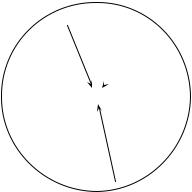
Figure 1.4 The value at site j may be modelled as a weighted sum of the influences of other sites i located within the zone of influence of the process generating the autocorrelation (large circle).
 i2
i2
 i3 i1
i3 i1 


 j
j
i4 
1 — Types of spatial structures
A spatial structure may appear in a variable y because the process that has produced the values of y is spatial and has generated autocorrelation in the data; or it may be caused by dependence of y upon one or several causal variables x which are spatially structured; or both. The spatially-structured causal variables x may be explicitly identified in the model, or not; see Table 13.3.
Autocorre- • Model 1: autocorrelation — The value yj observed at site j on the geographic surface lation is assumed to be the overall mean of the process ( y) plus a weighted sum of the
centred values ( yi – y) at surrounding sites i, plus an independent error term εj :
y j = y + Σ f ( yi – y) + ε j |
(1.1) |
The yi’s are the values of y at other sites i located within the zone of spatial influence of the process generating the autocorrelation (Fig. 1.4). The influence of neighbouring sites may be given, for instance, by weights wi which are function of the distance between sites i and j (eq. 13.19); other functions may be used. The total error term is [Σ f ( yi – y) + ε j] ; it contains the autocorrelated component of variation. As written here, the model assumes stationarity (Subsection 13.1.1). Its equivalent in time series analysis is the autoregressive (AR) response model (eq. 12.30).
Spatial • Model 2: spatial dependence — If one can assume that there is no autocorrelation in dependence the variable of interest, the spatial structure may result from the influence of some
explanatory variable(s) exhibiting a spatial structure. The model is the following:
y j = y + f (explanatory variables) + ε j |
(1.2) |
where yj is the value of the dependent variable at site j and εj is an error term whose value is independent from site to site. In such a case, the spatial structure, called “trend”, may be filtered out by trend surface analysis (Subsection 13.2.1), by the
12 |
Complex ecological data sets |
|
|
method of spatial variate differencing (see Cliff & Ord 1981, Section 7.4), or by some equivalent method in the case of time series (Chapter 12). The significance of the relationship of interest (e.g. correlation, presence of significant groups) is tested on the
Detrending detrended data. The variables should not be detrended, however, when the spatial structure is of interest in the study. Chapter 13 describes how spatial structures may be studied and decomposed into fractions that may be attributed to different hypothesized causes (Table 13.3).
It is difficult to determine whether a given observed variable has been generated under model 1 (eq. 1.1) or model 2 (eq. 1.2). The question is further discussed in Subsection 13.1.2 in the case of gradients (“false gradients” and “true gradients”).
More complex models may be written by combining autocorrelation in variable y (model 1) and the effects of causal variables x (model 2), plus the autoregressive structures of the various x’s. Each parameter of these models may be tested for significance. Models may be of various degrees of complexity, e.g. simultaneous AR model, conditional AR model (Cliff & Ord, 1981, Sections 6.2 and 6.3; Griffith, 1988, Chapter 4).
Spatial structures may be the result of several processes acting at different spatial scales, these processes being independent of one another. Some of these — usually the intermediate or fine-scale processes — may be of interest in a given study, while other processes may be well-known and trivial, like the broad-scale effects of tides or worldwide climate gradients.
2 — Tests of statistical significance in the presence of autocorrelation
Autocorrelation in a variable brings with it a statistical problem under the model-based approach (Section 1.0): it impairs the ability to perform standard statistical tests of hypotheses (Section 1.2). Let us consider an example of spatially autocorrelated data. The observed values of an ecological variable of interest — for example, species composition — are most often influenced, at any given site, by the structure of the species assemblages at surrounding sites, because of contagious biotic processes such as growth, reproduction, mortality and migration. Make a first observation at site A and a second one at site B located near A. Since the ecological process is understood to some extent, one can assume that the data are spatially autocorrelated. Using this assumption, one can anticipate to some degree the value of the variable at site B before the observation is made. Because the value at any one site is influenced by, and may be at least partly forecasted from the values observed at neighbouring sites, these values are not stochastically independent of one another.
The influence of spatial autocorrelation on statistical tests may be illustrated using the correlation coefficient (Section 4.2). The problem lies in the fact that, when the two variables under study are positively autocorrelated, the confidence interval, estimated by the classical procedure around a Pearson correlation coefficient (whose calculation assumes independent and identically distributed error terms for all observations), is
Autocorrelation and spatial structure |
13 |
|
|
r
-1
Confidence intervals of a correlation coefficient
0 |
|
|
+1 |
|||||||
|
||||||||||
|
|
|
|
|
|
|
|
|
|
Confidence interval corrected for |
|
|
|
|
|
|
|
|
|
spatial autocorrelation: r is not |
|
|
|
|
|
|
|
|
|
|
||
|
|
|
|
|
|
|
|
|
|
significantly different from zero |
|
|
|
|
|
|
|
|
Confidence interval computed |
||
|
|
|
|
|
|
|
|
|
|
from the usual tables: r ≠ 0 * |
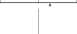
Figure 1.5 Effect of positive spatial autocorrelation on tests of correlation coefficients; * means that the coefficient is declared significantly different from zero in this example.
narrower than it is when calculated correctly, i.e. taking autocorrelation into account. The consequence is that one would declare too often that correlation coefficients are significantly different from zero (Fig. 1.5; Bivand, 1980). All the usual statistical tests, nonparametric and parametric, have the same behaviour: in the presence of positive autocorrelation, computed test statistics are too often declared significant under the null hypothesis. Negative autocorrelation may produce the opposite effect, for instance in analysis of variance (ANOVA).
The effects of autocorrelation on statistical tests may also be examined from the point of view of the degrees of freedom. As explained in Box 1.2, in classical statistical testing, one degree of freedom is counted for each independent observation, from which the number of estimated parameters is subtracted. The problem with autocorrelated data is their lack of independence or, in other words, the fact that new observations do not each bring with them one full degree of freedom, because the values of the variable at some sites give the observer some prior knowledge of the values the variable should take at other sites. The consequence is that new observations cannot be counted for one full degree of freedom. Since the size of the fraction they bring with them is difficult to determine, it is not easy to know what the proper reference distribution for the test should be. All that is known for certain is that positive autocorrelation at short distance distorts statistical tests (references in the next paragraph), and that this distortion is on the “liberal” side. This means that, when positive spatial autocorrelation is present in the small distance classes, the usual statistical tests too often lead to the decision that correlations, regression coefficients, or differences among groups are significant, when in fact they may not be.
This problem has been well documented in correlation analysis (Bivand, 1980; Cliff & Ord, 1981, §7.3.1; Clifford et al., 1989; Haining, 1990, pp. 313-330; Dutilleul, 1993a), linear regression (Cliff & Ord, 1981, §7.3.2; Chalmond, 1986; Griffith, 1988, Chapter 4; Haining, 1990, pp. 330-347), analysis of variance (Crowder & Hand, 1990; Legendre et al., 1990), and tests of normality (Dutilleul & Legendre, 1992). The problem of estimating the confidence interval for the mean when the sample data are
14 |
Complex ecological data sets |
|
|
Degrees of freedom |
Box 1.2 |
Statistical tests of significance often call upon the concept of degrees of freedom. A formal definition is the following: “The degrees of freedom of a model for expected values of random variables is the excess of the number of variables [observations] over the number of parameters in the model” (Kotz & Johnson, 1982).
In practical terms, the number of degrees of freedom associated with a statistic is equal to the number of its independent components, i.e. the total number of components used in the calculation minus the number of parameters one had to estimate from the data before computing the statistic. For example, the number of degrees of freedom associated with a variance is the number of observations minus one (noted ν = n – 1): n components ( xi – x) are used in the calculation, but one degree of freedom is lost because the mean of the statistical population is estimated from the sample data; this is a prerequisite before estimating the variance.
There is a different t distribution for each number of degrees of freedom. The same is true for the F and χ2 families of distributions, for example. So, the number of degrees of freedom determines which statistical distribution, in these families (t, F, or χ2), should be used as the reference for a given test of significance. Degrees of freedom are discussed again in Chapter 6 with respect to the analysis of contingency tables.
autocorrelated has been studied by Cliff & Ord (1975, 1981, §7.2) and Legendre & Dutilleul (1991).
When the presence of spatial autocorrelation has been demonstrated, one may wish to remove the spatial dependency among observations; it would then be valid to compute the usual statistical tests. This might be done, in theory, by removing observations until spatial independence is attained; this solution is not recommended because it entails a net loss of information which is often expensive. Another solution is detrending the data (Subsection 1); if autocorrelation is part of the process under study, however, this would amount to throwing out the baby with the water of the bath. It would be better to analyse the autocorrelated data as such (Chapter 13), acknowledging the fact that autocorrelation in a variable may result from various causal mechanisms (physical or biological), acting simultaneously and additively.
The alternative for testing statistical significance is to modify the statistical method in order to take spatial autocorrelation into account. When such a correction is available, this approach is to be preferred if one assumes that autocorrelation is an intrinsic part of the ecological process to be analysed or modelled.
Autocorrelation and spatial structure |
15 |
|
|
Corrected tests rely on modified estimates of the variance of the statistic, and on corrected estimates of the effective sample size and of the number of degrees of freedom. Simulation studies are used to demonstrate the validity of the modified tests. In these studies, a large number of autocorrelated data sets are generated under the null hypothesis (e.g. for testing the difference between two means, pairs of observations are drawn at random from the same simulated, autocorrelated statistical distribution, which corresponds to the null hypothesis of no difference between population means) and tested using the modified procedure; this experiment is repeated a large number of times to demonstrate that the modified testing procedure leads to the nominal confidence level.
Cliff & Ord (1973) have proposed a method for correcting the standard error of parameter estimates for the simple linear regression in the presence of autocorrelation. This method was extended to linear correlation, multiple regression, and t-test by Cliff & Ord (1981, Chapter 7: approximate solution) and to the one-way analysis of variance by Griffith (1978, 1987). Bartlett (1978) has perfected a previously proposed method of correction for the effect of spatial autocorrelation due to an autoregressive process in randomized field experiments, adjusting plot values by covariance on neighbouring plots before the analysis of variance; see also the discussion by Wilkinson et al. (1983) and the papers of Cullis & Gleeson (1991) and Grondona & Cressis (1991). Cook & Pocock (1983) have suggested another method for correcting multiple regression parameter estimates by maximum likelihood, in the presence of spatial autocorrelation. Using a different approach, Legendre et al. (1990) have proposed a permutational method for the analysis of variance of spatially autocorrelated data, in the case where the classification criterion is a division of a territory into nonoverlapping regions and one wants to test for differences among these regions.
A step forward was proposed by Clifford et al. (1989), who tested the significance of the correlation coefficient between two spatial processes by estimating a modified number of degrees of freedom, using an approximation of the variance of the correlation coefficient computed on data. Empirical results showed that their method works fine for positive autocorrelation in large samples. Dutilleul (1993a) generalized the procedure and proposed an exact method to compute the variance of the sample covariance; the new method is valid for any sample size.
Major contributions to this topic are found in the literature on time series analysis, especially in the context of regression modelling. Important references are Cochrane & Orcutt (1949), Box & Jenkins (1976), Beach & MacKinnon (1978), Harvey & Phillips (1979), Chipman (1979), and Harvey (1981).
When methods specifically designed to handle spatial autocorrelation are not available, it is sometimes possible to rely on permutation tests, where the significance is determined by random reassignment of the observations (Section 1.2). Special permutational schemes have been developed that leave autocorrelation invariant; examples are found in Besag & Clifford (1989), Legendre et al. (1990) and ter Braak
16 |
Complex ecological data sets |
|
|
(1990, section 8). For complex problems, such as the preservation of spatial or temporal autocorrelation, the difficulty of the permutational method is to design an appropriate permutation procedure.
The methods of clustering and ordination described in Chapters 8 and 9 to study ecological structures do not rely on tests of statistical significance. So, they are not affected by the presence of spatial autocorrelation. The impact of spatial autocorrelation on numerical methods will be stressed wherever appropriate.
3 — Classical sampling and spatial structure
Random or systematic sampling designs have been advocated as a way of preventing the possibility of dependence among observations (Cochran 1977; Green 1979; Scherrer 1982). This was then believed to be a necessary and sufficient safeguard against violations of the independence of errors, which is a basic assumption of classical statistical tests. It is adequate, of course, when one is trying to estimate the parameters of a local population. In such a case, a random or systematic sample is suitable to obtain unbiased estimates of the parameters since, a priori, each point has the same probability of being included in the sample. Of course, the variance and, consequently, also the standard error of the mean increase if the distribution is patchy, but their estimates remain unbiased.
Even with random or systematic allocation of observations through space, observations may retain some degree of spatial dependence if the average distance between first neighbours is shorter than the zone of spatial influence of the underlying ecological phenomenon. In the case of broad-scale spatial gradients, no point is far enough to lie outside this zone of spatial influence. Correlograms and variograms (Chapter 13), combined with maps, are used to assess the magnitude and shape of autocorrelation present in data sets.
Classical books such as Cochran (1977) adequately describe the rules that should govern sampling designs. Such books, however, emphasize only the design-based inference (Section 1.0), and do not discuss the influence of spatial autocorrelation on the sampling design. At the present time, literature on this subject seems to be only available in the field of geostatistics, where important references are: David (1977, Ch. 13), McBratney & Webster (1981), McBratney et al. (1981), Webster & Burgess (1984), Borgman & Quimby (1988), and François-Bongarçon (1991).
Ecologists interested in designing field experiments should read the paper of Dutilleul (1993b), who discusses how to accommodate an experiment to spatially Heterogeheterogeneous conditions. The concept of spatial heterogeneity is discussed at some
neity length in the multi-author book edited by Kolasa & Pickett (1991), in the review paper of Dutilleul & Legendre (1993), and in Section 13.0.
Statistical testing by permutation |
17 |
|
|
1.2 Statistical testing by permutation
|
The role of a statistical test is to decide whether some parameter of the reference |
|
population may take a value assumed by hypothesis, given the fact that the |
|
corresponding statistic, whose value is estimated from a sample of objects, may have a |
Statistic |
somewhat different value. A statistic is any quantity that may be calculated from the |
|
data and is of interest for the analysis (examples below); in tests of significance, a |
|
statistic is called test statistic or test criterion. The assumed value of the parameter |
|
corresponding to the statistic in the reference population is given by the statistical null |
|
hypothesis (written H0), which translates the biological null hypothesis into numerical |
|
terms; it often negates the existence of the phenomenon that the scientists hope to |
|
evidence. The reasoning behind statistical testing directly derives from the scientific |
|
method; it allows the confrontation of experimental or observational findings to |
|
intellectual constructs that are called hypotheses. |
|
Testing is the central step of inferential statistics. It allows one to generalize the |
|
conclusions of statistical estimation to some reference population from which the |
|
observations have been drawn and that they are supposed to represent. Within that |
|
context, the problem of multiple testing is too often ignored (Box. 1.3). Another |
|
legitimate section of statistical analysis, called descriptive statistics, does not rely on |
|
testing. The methods of clustering and ordination described in Chapters 8 and 9, for |
|
instance, are descriptive multidimensional statistical methods. The interpretation |
|
methods described in Chapters 10 and 11 may be used in either descriptive or |
|
inferential mode. |
|
1 — Classical tests of significance |
|
Consider, for example, a correlation coefficient (which is the statistic of interest in |
|
correlation analysis) computed between two variables (Chapter 4). When inference to |
Null |
the statistical population is sought, the null hypothesis is often that the value of the |
hypothesis |
correlation parameter (ρ, rho) in the statistical population is zero; the null hypothesis |
|
may also be that ρ has some value other than zero, given by the ecological hypothesis. |
|
To judge of the validity of the null hypothesis, the only information available is an |
|
estimate of the correlation coefficient, r, obtained from a sample of objects drawn from |
|
the statistical population. (Whether the observations adequately represent the |
|
statistical population is another question, for which the readers are referred to the |
|
literature on sampling design.) We know, of course, that a sample is quite unlikely to |
|
produce a parameter estimate which is exactly equal to the true value of the parameter |
|
in the statistical population. A statistical test tries to answer the following question: |
|
given a hypothesis stating, for example, that ρ = 0 in the statistical population and the |
|
fact that the estimated correlation is, say, r = 0.2, is it justified to conclude that the |
|
difference between 0.2 and 0.0 is due to sampling error? |
|
The choice of the statistic to be tested depends on the problem at hand. For |
|
instance, in order to find whether two samples may have been drawn from the same |

18 |
Complex ecological data sets |
|
|
Multiple testing |
Box 1.3 |
When several tests of significance are carried out simultaneously, the probability of a type I error becomes larger than the nominal value α. For example, when analysing a correlation matrix involving 5 variables, 10 tests of significance are carried out simultaneously. For randomly generated data, there is a probability p = 0.40 of rejecting the null hypothesis at least once over 10 tests, at the nominal α = 0.05 level; this can easily be computed from the binomial distribution. So, when conducting multiple tests, one should perform a global test of significance in order to determine whether there is any significant value at all in the set.
The first approach is Fisher's method for combining the probabilities pi obtained from k independent tests of significance. The value –2Σ ln(pi) is distributed as χ2 with 2k degrees of freedom if the null hypothesis is true in all k tests (Fisher, 1954; Sokal & Rohlf, 1995).
Another approach is the Bonferroni correction for k independent tests: replace the significance level, say α = 0.05, by an adjusted level α' = α/k, and compare probabilities pi to α'. This is equivalent to adjusting individual p-values pi to p'i = kpi and comparing p'i to the unadjusted significance level α. While appropriate to test the null hypothesis for the whole set of simultaneous hypotheses (i.e. reject H0 for the whole set of k hypotheses if the smallest unadjusted p-value in the set is less than or equal to α/k), the Bonferroni method is overly conservative and often leads to rejecting too few individual hypotheses in the set k.
Several alternatives have been proposed in the literature; see Wright (1992) for a review. For non-independent tests, Holm’s procedure (1979) is nearly as simple to carry out as the Bonferroni adjustment and it is much more powerful, leading to rejecting the null hypothesis more often. It is computed as follows. (1) Order the p-values from left to right so that p1 ≤ p2 ≤ … ≤ pi … ≤ pk. (2) Compute adjusted probability values p'i = (k – i + 1)pi ; adjusted probabilities may be larger than 1. (3) Proceeding from left to right, if an adjusted p-value in the ordered series is smaller than the one occurring at its left, make the smallest equal to the largest one. (4) Compare each adjusted p'i to the unadjusted α significance level and make the statistical decision. The procedure could be formulated in terms of successive corrections to the α significance level, instead of adjustments to individual probabilities.
An even more powerful solution is that of Hochberg (1988) which has the desired overall (“experimentwise”) error rate α only for independent tests (Wright, 1992). Only step (3) differs from Holm’s procedure: proceeding this time from right to left, if an adjusted p-value in the ordered series is smaller than the one at its left, make the largest equal to the smallest one. Because the adjusted probabilities form a nondecreasing series, both of these procedures present the properties (1) that a hypothesis in the ordered series cannot be rejected unless all previous hypotheses in the series have also been rejected and (2) that equal p-values receive equal adjusted p-values. Hochberg’s method presents the further characteristic that no adjusted p-value can be larger than the largest unadjusted p-value or exceed 1. More complex and powerful procedures are explained by Wright (1992).
For some applications, special procedures have been developed to test a whole set of statistics. An example is the test for the correlation matrix R (eq. 4.14, end of Section 4.2).

|
Statistical testing by permutation |
19 |
|
|
|
|
statistical population or from populations with equal means, one would choose a |
|
Pivotal |
statistic measuring the difference between the two sample means (x1 – x2 ) or, |
|
preferably, a pivotal form like the usual t statistic used in such tests; a pivotal statistic |
||
statistic |
has a distribution under the null hypothesis which remains the same for any value of |
|
|
the measured effect (here, x1 – x2 ). In the same way, the slope of a regression line is |
|
|
described by the slope parameter of the linear regression equation, which is assumed, |
|
|
under the null hypothesis, to be either zero or some other value suggested by |
|
|
ecological theory. The test statistic describes the difference between the observed and |
|
|
hypothesized value of slope; the pivotal form of this difference is a t or F statistic. |
|
Alternative |
Another aspect of a statistical test is the alternative hypothesis (H1), which is also |
|
hypothesis |
imposed by the ecological problem at hand. H1 is the opposite of H0, but there may be |
|
several statements that represent some opposite of H0. In correlation analysis for instance, if one is satisfied to determine that the correlation coefficient in the reference population (ρ) is significantly different from zero in either the positive or the negative direction, meaning that some linear relationship exists between two variables, then a two-tailed alternative hypothesis is stated about the value of the parameter in the statistical population: ρ ≠ 0. On the contrary, if the ecological phenomenon underlying the hypothesis imposes that a relationship, if present, should have a given sign, one formulates a one-tailed hypothesis. For instance, studies on the effects of acid rain are motivated by the general paradigm that acid rain, which lowers the pH, has a negative effect on terrestrial and aquatic ecosystems. In a study of the correlation between pH and diversity, one would formulate the following hypothesis H1: pH and diversity are positively correlated (i.e. low pH is associated with low diversity; H1: ρ > 0). Other situations would call for a different alternative hypothesis, symbolized by H1: ρ < 0.
The expressions one-tailed and two-tailed refer to the fact that, in a two-tailed test, one would look in both tails of the reference statistical distribution for values as extreme as, or more extreme than the reference value of the statistic (i.e. the one computed from the actual data). In a correlation study for instance, where the reference distribution (t) for the test statistic is symmetric about zero, the probability of the null hypothesis in a two-tailed test is given by the proportion of values in the t distribution which are, in absolute value, as large as, or larger than the absolute value of the reference statistic. In a one-tailed test, one would look only in the tail corresponding to the sign given by the alternative hypothesis; for instance, for the proportion of values in the t distribution which are as large as or larger than the signed value of the reference t statistic, for a test in the right-hand tail (Η1: ρ > 0).
In standard statistical tests, the test statistic computed from the data is referred to one of the usual statistical distributions printed in books or computed by some appropriate computer software; the best-known are the z, t, F and χ2 distributions. This, however, can only be done if certain assumptions are met by the data, depending on the test. The most commonly encountered are the assumptions of normality of the variable(s) in the reference population, homoscedasticity (Box 1.4) and independence of the observations (Box 1.1). Refer to Siegel (1956, Chapter 2), Siegel & Castellan

20 |
Complex ecological data sets |
|
|
(1988, Chapter 2), or Snedecor & Cochran (1967, Chapter 1), for concise yet clear classical exposés of the concepts related to statistical testing.
2 — Permutation tests
The method of permutation, also called randomization, is a very general approach to testing statistical hypotheses. Following Manly (1997), permutation and randomization are considered synonymous in the present book, although permutation Randomimay also be considered to be the technique by which the principle of randomization is
zation applied to data during permutation tests. Other points of view are found in the literature. For instance, Edgington (1995) considers that a randomization test is a permutation test based on randomization. A different although related meaning of randomization refers to the random assignment of replicates to treatments in experimental designs.
Permutation testing can be traced back to at least Fisher (1935, Chapter 3). Instead of comparing the actual value of a test statistic to a standard statistical distribution, the reference distribution is generated from the data themselves, as described below; other randomization methods are mentioned at the end of the present Section. Permutation provides an efficient approach to testing when the data do not conform to the distributional assumptions of the statistical method one wants to use (e.g. normality). Permutation testing is applicable to very small samples, like nonparametric tests. It does not resolve problems of independence of the observations, however. Nor does the method solve distributional problems that are linked to the hypothesis subjected to a test*. Permutation remains the method of choice to test novel or other statistics whose distributions are poorly known. Furthermore, results of permutation tests are valid even with observations that are not a random sample of some statistical population; this point is further discussed in Subsection 4. Edgington (1995) and Manly (1997) have written excellent introductory books about the method. A short account is given by Sokal & Rohlf (1995) who prefer to use the expression “randomization test”. Permutation tests are used in several Chapters of the present book.
The speed of modern computers would allow users to perform any statistical test using the permutation method. The chief advantage is that one does not have to worry about distributional assumptions of classical testing procedures; the disadvantage is the amount of computer time required to actually perform a large number of permutations, each one being followed by recomputation of the test statistic. This disadvantage vanishes as faster computers come on the market. As an example, let us
* For instance, when studying the differences among sample means (two groups: t-test; several groups: F test of ANOVA), the classical Behrens-Fisher problem (Robinson, 1982) reminds us that two null hypotheses are tested simultaneously by these methods, i.e. equality of the means and equality of the variances. Testing the t or F statistics by permutations does not change the dual aspect of the null hypothesis; in particular, it does not allow one to unambiguously test the equality of the means without checking first the equality of the variances using another, more specific test (two groups: F ratio; several groups: Bartlett’s test of equality of variances).

Statistical testing by permutation |
21 |
|
|
consider the situation where the significance of a correlation coefficient between two variables, x1 and x2, is to be tested.
Hypotheses
•H0: The correlation between the variables in the reference population is zero (ρ = 0).
•For a two-tailed test, H1: ρ ≠ 0.
•Or for a one-tailed test, either H1: ρ > 0, or H1: ρ < 0, depending on the ecological hypothesis.
Test statistic |
|
|
• Compute the |
Pearson |
correlation coefficient r. Calculate the pivotal statistic |
t = n – 2 [r ⁄ |
1 – r2] |
(eq. 4.13; n is the number of observations) and use it as the |
reference value in the remainder of the test.
In this specific case, the permutation test results would be the same using either r or t as the test statistic, because t is a monotonic function of r for any constant value of n; r and t are “equivalent statistics for permutation tests”, sensu Edgington (1995). This is not always the case. When testing a partial regression coefficient in multiple regression, for example, the test should not be based on the distribution of permuted partial regression coefficients because they are not monotonic to the corresponding partial t statistics. The partial t should be preferred because it is pivotal and, hence, it is expected to produce correct type I error.
Considering a pair of equivalent test statistics, one could choose the statistic which is the simplest to compute if calculation time would otherwise be longer in an appreciable way. This is not the case in the present example: calculating t involves a single extra line in the computer program compared to r. So the test is conducted using the usual t statistic.
Distribution of the test statistic
The argument invoked to construct a null distribution for the statistic is that, if the null hypothesis is true, all possible pairings of the two variables are equally likely to occur. The pairing found in the observed data is just one of the possible, equally likely pairings, so that the value of the test statistic for the unpermuted data should be typical, i.e. located in the central part of the permutation distribution.
• It is always the null hypothesis which is subjected to testing. Under H0, the rows of x1 are seen as “exchangeable” with one another if the rows of x2 are fixed, or conversely. The observed pairing of x1 and x2 values is due to chance alone; accordingly, any value of x1 could have been paired with any value of x2.
22 |
Complex ecological data sets |
|
|
•A realization of H0 is obtained by permuting at random the values of x1 while holding the values of x2 fixed, or the opposite (which would produce, likewise, a random pairing of values). Recompute the value of the correlation coefficient and the associated t statistic for the randomly paired vectors x1 and x2, obtaining a value t*.
•Repeat this operation a large number of times (say, 999 times). The different permutations produce a set of values t* obtained under H0.
•Add to these the reference value of the t statistic, computed for the unpermuted
vectors. Since H0 is being tested, this value is considered to be one that could be obtained under H0 and, consequently, it should be added to the reference distribution (Hope, 1968; Edgington, 1995; Manly, 1997). Together, the unpermuted and permuted
values form an estimate of the sampling distribution of t under H0, to be used in the next step.
Statistical decision
• As in any other statistical test, the decision is made by comparing the reference value of the test statistic (t) to the reference distribution obtained under H0. If the reference value of t is typical of the values obtained under the null hypothesis (which states that there is no relationship between x1 and x2), H0 cannot be rejected; if it is unusual, being too extreme to be considered a likely result under H0, H0 is rejected and the alternative hypothesis is considered to be a more likely explanation of the data.
Significance • The significance level of a statistic is the proportion of values that are as extreme as, level or more extreme than the test statistic in the reference distribution, which is either obtained by permutations or found in a table of the appropriate statistical distribution.
The level of significance should be regarded as “the strength of evidence against the null hypothesis” (Manly, 1997).
3 — Numerical example
Let us consider the following case of two variables observed over 10 objects:
x1 |
–2.31 |
1.06 |
0.76 |
1.38 |
–0.26 |
1.29 |
–1.31 |
0.41 |
–0.67 |
–0.58 |
x2 |
–1.08 |
1.03 |
0.90 |
0.24 |
–0.24 |
0.76 |
–0.57 |
–0.05 |
–1.28 |
1.04 |
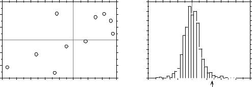
These values were drawn at random from a positively correlated bivariate normal distribution, as shown in Fig. 1.6a. Consequently, they would be suitable for parametric testing. So, it is interesting to compare the results of a permutation test to the usual parametric t-test of the correlation coefficient. The statistics and associated probabilities for this pair of variables, for ν = (n – 2) = 8 degrees of freedom, are:
r = 0.70156, t = 2.78456, n = 10:
prob (one-tailed) = 0.0119, prob (two-tailed) = 0.0238.
Statistical testing by permutation |
23 |
|
|
Variable 2
1.5 |
|
|
|
|
|
|
|
|
160 |
|
|
|
|
|
|
|
1.0 |
(a) |
|
|
|
|
|
|
|
140 |
(b) |
|
|
|
|
|
|
|
|
|
|
|
|
|
|
|
|
|
|
|
|
|||
|
|
|
|
|
|
|
|
|
120 |
|
|
|
|
|
|
|
0.5 |
|
|
|
|
|
|
|
Frequency |
100 |
|
|
|
|
|
|
|
|
|
|
|
|
|
|
|
|
|
|
|
|
|
|
||
|
|
|
|
|
|
|
|
60 |
|
|
|
|
|
|
|
|
0.0 |
|
|
|
|
|
|
|
|
80 |
|
|
|
|
|
|
|
–0.5 |
|
|
|
|
|
|
|
|
|
|
|
|
|
|
|
|
|
|
|
|
|
|
|
|
|
40 |
|
|
|
|
|
|
|
–1.0 |
|
|
|
|
|
|
|
|
20 |
|
|
|
|
|
|
|
|
|
|
|
|
|
|
|
|
|
|
|
|
|
|
|
|
–1.5 |
|
|
|
|
|
|
|
|
0 |
|
|
|
|
|
|
|
–2.5 |
–2.0 |
–1.5 |
–1.0 |
–0.5 |
0.0 |
0.5 |
1.0 |
1.5 |
–6 |
–4 |
–2 |
0 |
2 |
4 |
6 |
8 |
|
|
|
Variable 1 |
|
|
|
|
|
|
t statistic |
2.78456 |
|
|
|||
Figure 1.6 |
(a) Positions of the 10 points of the numerical example with respect to variables x1 and x2. |
|
(b) Frequency histogram of the (1 + 999) permutation results (t statistic for correlation |
|
coefficient); the reference value obtained for the points in (a), t = 2.78456, is also shown. |
There are 10! = 3.6288 106 possible permutations of the 10 values of variable x1 (or x2). Here, 999 of these permutations were generated using a random permutation algorithm; they represent a random sample of the 3.6288 106 possible permutations. The computed values for the test statistic (t) between permuted x1 and fixed x2 have the distribution shown in Fig. 1.6b; the reference value, t = 2.78456, has been added to this distribution. The permutation results are summarized in the following table, where ‘|t|’ is the (absolute) reference value of the t statistic ( t = 2.78456) and ‘t*’ is a value obtained after permutation. The absolute value of the reference t is used in the table to make it a general example, because there are cases where t is negative.
|
t* < – t |
t* = – t |
– t < t* < t |
t* = t |
t* > t |
|
|
|
|
|
|
Statistic t |
8 |
0 |
974 |
1† |
17 |
† This count corresponds to the reference t value added to the permutation results.
For a one-tailed test (in the right-hand tail in this case, since H1: ρ > 0), one counts how many values in the permutational distribution of the statistic are equal to, or larger than, the reference value (t* ≥ t; there are 1 + 17 = 18 such values in this case). This is the only one-tailed hypothesis worth considering, because the objects are known in this case to have been drawn from a positively correlated distribution. A one-tailed test in the left-hand tail (H1: ρ < 0) would be based on how many values in the permutational distribution are equal to, or smaller than, the reference value (t* ≤ t, which are 8 + 0 + 974 +1 = 983 in the example). For a two-tailed test, one counts all values that are as extreme as, or more extreme than the reference value in both tails of the distribution ( t* ≥ t , which are 8 + 0 + 1 + 17 = 26 in the example).
24 |
Complex ecological data sets |
|
|
|
Probabilities associated with these distributions are computed as follows, for a one- |
|
tailed and a two-tailed test (results using the t statistic would be the same): |
|
One-tailed test [H0: ρ = 0; H1: ρ > 0]: |
|
prob (t* ≥ 2.78456) = (1 + 17)/1000 = 0.018 |
|
Two-tailed test [H0: ρ = 0; H1: ρ ≠ 0]: |
|
prob( t* ≥ 2.78456) = (8 + 0 + 1 + 17)/1000 = 0.026 |
|
Note how similar the permutation results are to the results obtained from the |
|
classical test, which referred to a table of Student t distributions. The observed |
|
difference is partly due to the small number of pairs of points (n = 10) sampled at |
|
random from the bivariate normal distribution, with the consequence that the data set |
|
does not quite conform to the hypothesis of normality. It is also due, to a certain extent, |
|
to the use of only 999 permutations, sampled at random among the 10! possible |
|
permutations. |
|
4 — Remarks on permutation tests |
|
In permutation tests, the reference distribution against which the statistic is tested is |
|
obtained by randomly permuting the data under study, without reference to any |
|
statistical population. The test is valid as long as the reference distribution has been |
|
generated by a procedure related to a null hypothesis that makes sense for the problem |
|
at hand, irrespective of whether or not the data set is representative of a larger |
|
statistical population. This is the reason why the data do not have to be a random |
|
sample from some larger statistical population. The only information the permutation |
|
test provides is whether the pattern observed in the data is likely, or not, to have arisen |
|
by chance. For this reason, one may think that permutation tests are not as “good” or |
|
“interesting” as classical tests of significance because they might not allow one to infer |
|
conclusions that apply to a statistical population. |
|
A more pragmatic view is that the conclusions of permutation tests may be |
|
generalized to a reference population if the data set is a random sample of that |
|
population. Otherwise, they allow one to draw conclusions only about the particular |
|
data set, measuring to what extent the value of the statistic is “usual” or “unusual” with |
|
respect to the null hypothesis implemented in the permutation procedure. Edgington |
|
(1995) and Manly (1997) further argue that data sets are very often not drawn at |
|
random from statistical populations, but simply consist of observations which happen |
|
to be available for study. The generalization of results, in classical as well as |
|
permutation tests, depends on the degree to which the data were actually drawn at |
|
random, or are equivalent to a sample drawn at random, from a reference population. |
Complete |
For small data sets, one can compute all possible permutations in a systematic way |
permutation |
and obtain the complete permutation distribution of the statistic; an exact or complete |
test |
permutation test is obtained. For large data sets, only a sample of all possible |
|
permutations may be computed because there are too many. When designing a |
|
Statistical testing by permutation |
25 |
|
|
|
Sampled |
sampled permutation test, it is important to make sure that one is using a uniform |
|
permutation |
random generation algorithm, capable of producing all possible permutations with |
|
test |
equal probabilities (Furnas, 1984). Computer programs use procedures that produce |
|
|
random permutations of the data; these in turn call the ‘Random’ function of computer |
|
|
languages. Such a procedure is described in Section 5.8 of Manly’s book (1997). |
|
|
Random permutation subprograms are also available in subroutine libraries. |
|
|
The case of the correlation coefficient has shown how the null hypothesis guided |
|
|
the choice of an appropriate permutation procedure, capable of generating realizations |
|
|
of this null hypothesis. A permutation test for the difference between the means of two |
|
|
groups would involve random permutations of the objects between the two groups |
|
|
instead of random permutations of one variable with respect to the other. The way of |
|
|
permuting the data depends on the null hypothesis to be tested. |
|
|
Some tests may be reformulated in terms of some other tests. For example, the t- |
|
|
test of equality of means is equivalent to a test of the correlation between the vector of |
|
|
observed values and a vector assigning the observations to group 1 or 2. The same |
|
|
value of t and probability (classical or permutational) are obtained using both methods. |
|
|
Simple statistical tests such as those of correlation coefficients or differences |
|
|
between group means may be carried out by permuting the original data, as in the |
|
|
example above. Problems involving complex relationships among variables may |
|
|
require permuting the residuals of some model instead of the raw data; model-based |
|
|
permutation is discussed in Subsection 11.3.2. The effect of a nominal covariable may |
|
Restricted |
be controlled for by restricted permutations, limited to the objects within the groups |
|
permu- |
defined by the covariable. This method is discussed in detail by Manly (1997). |
|
tations |
Applications are found in Brown & Maritz (1982; restrictions within replicated values |
|
|
in a multiple regression) and in Sokal et al. (1987; Mantel test), for instance. |
|
|
In sampled permutation tests, adding the reference value of the statistic to the |
|
|
distribution has the effect that it becomes impossible for the test to produce no value |
|
|
“as extreme as, or more extreme than the reference value”, as the standard expression |
|
|
goes. This way of computing the probability is biased, but it has the merit of being |
|
|
statistically valid (Edgington, 1995, Section 3.5). The precision of the probability |
|
|
estimate is the inverse of the number of permutations performed; for instance, after |
|
|
(999 + 1) permutations, the precision of the probability statement is 0.001. |
|
How many |
The number of permutations one should perform is always a trade-off between |
|
permu- |
precision and computer time. The more permutations the better, since probability |
|
tations? |
estimates are subject to error due to sampling the population of possible permutations |
|
|
(except in the rare cases of complete permutation tests), but it may be tiresome to wait |
|
|
for the permutation results when studying large data sets. In the case of the Mantel test |
|
|
(Section 10.5), Jackson & Somers (1989) recommend to compute 10000 to 100000 |
|
|
permutations in order to ensure the stability of the probability estimates. The following |
|
|
recommendation can be made. In exploratory analyses, 500 to 1000 permutations may |
|
|
be sufficient as a first contact with the problem. If the computed probability is close to |
|
26 |
Complex ecological data sets |
|
|
|
the preselected significance level, run more permutations. In any case, use more |
|
permutations (e.g. 10000) for final, published results. |
|
Interestingly, tables of critical values in nonparametric statistical tests for small |
|
sample sizes are based on permutations. The authors of these tables have computed |
|
how many cases can be found, in the complete permutation distribution, that are as |
|
extreme as, or more extreme than the computed value of the statistic. Hence, |
|
probability statements obtained from small-sample nonparametric tests are exact |
|
probabilities (Siegel, 1956). |
Monte Carlo |
Named after the famous casino of the principality of Monaco, Monte Carlo |
|
methods use random numbers to study either real data sets or the behaviour of |
|
statistical methods through simulations. Permutation tests are Monte Carlo methods |
|
because they use random numbers to randomly permute data. Other such methods are |
|
based on computer-intensive resampling. Among these are the jackknife (Tukey 1958; |
|
Sokal & Rohlf, 1995) and the bootstrap (Efron, 1979; Efron & Tibshirani, 1993; |
|
Manly, 1997). In these methods, the values used in each iteration to compute a statistic |
Jackknife |
form a subsample of the original data. In the jackknife, each subsample leaves out one |
Bootstrap |
of the original observations. In the bootstrap, each subsample is obtained by |
|
resampling the original sample with replacement; the justification is that resampling |
|
the original sample approximates a resampling of the original population. |
|
As an exercise, readers are invited to figure out how to perform a permutation test |
|
for the difference between the means of two groups of objects on which a single |
|
variable has been measured, using the t statistic; this would be equivalent to a t-test. A |
|
solution is given by Edgington (1995). Other types of permutation tests are discussed |
|
in Sections 7.3, 8.9, 10.2, 10.3, 10.5, 10.6, 11.3, 12.6, 13.1 and 13.3. |
1.3 Computers
Processing complex ecological data sets almost always requires the use of a computer, as much for the amount of data to be processed as for the fact that the operations to be performed are often tedious and repetitious. Work with computers is made simple by the statistical programs and packages available on microcomputers or on mainframes. For those who want to develop new methods, advanced programming languages such as S-PLUS or MATLAB , or the SAS Language, may be extremely useful. One may also complement programs written in one of the standard computer languages with statistical subprograms drawn from libraries such as NAG or IMSL , which are available at computing centres and contain subprograms for the numerical resolution of most common numerical problems. The ease of using computers, however, has two pitfalls that ecologists must bear in mind: the fact that computations are executed does not ensure (1) that the data satisfy the conditions required by the method, or (2) that the results produced by the computer are interpreted correctly in ecological terms.
Ecological descriptors |
27 |
|
|
In fact, ecologists must thoroughly master the numerical methods they use. If they do not, they may end up using approaches that are incompatible with their data, or selecting techniques that do not correspond to the goal of the research, or else interpreting the results either incompletely or incorrectly. The only role of the computer is to relieve the user of the calculations; it makes no appraisal of the pertinence of the selected method, or of the interpretation of the results. The aim of the following chapters is to provide ecologists with a guide to the use of the many numerical methods available, as well as the bases for translating, in ecological terms, the pages of numbers produced by computers. Indeed, a computer output is not in itself a conclusion and it will never replace ecologists for interpreting results.
Ten years ago, the statistical packages most widely available were BMDP (Biomedical Computer Programs), SPSS (Statistical Package for the Social Sciences) and SAS (Statistical Analysis System). Versions of these packages, originally developed for mainframe computers, are now available for microcomputers as well. A wide array of other programs and packages have also been developed for microcomputers, giving users a wide choice. The selection of a given package for a specific task may be guided by its availability for the user’s preferred machine, the methods it contains, and its computer-friendliness. In everyday work, ecologists rely nowadays on several packages, each specialized for specific tasks such as clustering, ordination, canonical analysis, time series analysis, spatial analysis, graphics, mapping, word processing, etc. While low-end microcomputers can perform most everyday tasks of data analysis, high-end machines or mainframes retain their usefulness to analyse large data bases or for permutation-based, computer-intensive statistical testing methods.
A review of the contents of the main statistical packages available on the market is beyond the scope of the present book, and would rapidly become obsolete. Such reviews may be found in statistical Journals, for instance The American Statistician,
Applied Statistics, or Statistics and Computing. Lists of programs for some of the more specialized fields of analysis will be provided in some chapters of this book.
Programs for all the numerical techniques described in the following chapters can be found in one or several packages. It is, therefore, much more efficient for ecologists to use these proven resources than to reprogram methods. Ecological data are, most of the time, so complex that a single analysis cannot extract all their useful information. Therefore, ecologists who judiciously use existing programs have access to a variety of numerical methods, which are needed to cover the wide range of ecological situations encountered in field studies.
1.4 Ecological descriptors
Descriptor |
Any ecological study, classical or numerical, is based on descriptors. In the present |
Variable |
text, the terms descriptor and variable will be used interchangeably. These refer to the |
28 |
Complex ecological data sets |
|
|
|
attributes, or characters (also called items in the social sciences, and profiles or |
|
features in the field of pattern recognition) used to describe or compare the objects of |
Object |
the study. The objects that ecologists compare are the sites, quadrats, observations, |
|
sampling units, individual organisms, or subjects which are defined a priori by the |
|
sampling design, before making the observations (Section 2.1). Observation units are |
|
often called “samples” by ecologists; the term sample is only used in this book to refer |
|
to a set of observations resulting from a sampling action or campaign. Objects may be |
|
called individuals or OTUs (Operational taxonomic units) in numerical taxonomy, |
|
OGUs (Operational geographic units) in biogeography, cases, patterns or items in the |
|
field of pattern recognition, etc. |
|
The descriptors, used to describe or qualify the objects, are the physical, chemical, |
|
ecological, or biological characteristics of these objects that are of interest for the |
|
study. In particular, biological species are descriptors of sites for ecologists; in |
|
(numerical) taxonomy on the contrary, the species are the objects of the study, and the |
|
sites where the species are observed or collected may be used by the taxonomist as |
|
descriptors of the species. It all depends on the variable defined a priori, which is fixed |
|
as object for the study. In ecology, sites are compared using the species they contain, |
|
there being no possibility of choosing the species, whereas taxonomists compare |
|
populations or other taxonomic entities obtained from a number of different sites. |
Descriptor |
A descriptor is a law of correspondence established by the researcher to describe and |
|
compare, on the same basis, all the objects of the study. This definition applies to all types of |
|
descriptors discussed below (Table 1.2). The fundamental property of a descriptor, as understood |
|
in the present book, is that it distributes the objects among non-overlapping states. Each |
|
descriptor must, therefore, operate like a law that associates with each object in the group under |
|
study one and only one element of a set of distinguishable states that belong to the descriptor. |
Descriptor |
The states that constitute a descriptor must necessarily be mutually exclusive. In |
state |
other words, two different states of the same descriptor must not be applicable to the |
|
same object. Descriptors, on the contrary, do not have to be independent of one another |
|
(see Box 1.1: independent descriptors). In Chapter 6, it will be seen that the |
|
information contained in one descriptor may partially or totally overlap with the |
|
information in an other. In Chapters 8 and 9, such redundant or correlated information |
|
will be used as the basis for the clustering or ordination of ecological objects. |
|
1 — Mathematical types of descriptor |
|
The states which form a descriptor — that is, the qualities observed or determined |
|
on the objects — may be of a qualitative or quantitative nature, so that descriptors may |
|
be classified into several types. In ecology, a descriptor may be biological (presence, |
|
abundance, or biomass of different species), physical, chemical, geological, |
|
geographical, temporal, climatic, etc. Table 1.2 presents a classification of descriptors |
|
according to their mathematical types. This classification is, therefore, independent of |
|
the particular discipline to which the descriptors belong. The mathematical type of a |
|
descriptor determines the type of numerical processing which can be applied to it. For |

Ecological descriptors |
29 |
|
|
Table 1.2 |
The different mathematical types of descriptors. |
|
|||
|
|
|
|
|
|
|
Descriptor types |
Examples |
|||
|
|
|
|
|
|
|
Binary (two states, presence-absence) |
Species present or absent |
|||
|
Multi-state (many states) |
|
|||
|
|
Nonordered (qualitative, nominal, attributes) |
Geological group |
||
|
|
||||
|
|
Ordered |
|
||
|
|
|
Semiquantitative (rank-ordered, ordinal) |
Importance or abundance scores |
|
|
|
|
|||
|
|
|
Quantitative (metric, measurement) |
|
|
|
|
|
|
Discontinuous (meristic, discrete) |
Equidistant abundance classes |
|
|
|
|
||
|
|
|
|
Continuous |
Temperature, length |
|
|
|
|
|
|
|
|
|
|
|
|
example, parametric correlations (Pearson’s r) may be calculated between quantitative descriptors, while nonparametric correlations (such as Kendall’s τ) may be used on ordered but not necessarily quantitative descriptors, as long as their relationship is monotonic. To measure the dependence among descriptors that are not in monotonic relationship, or among qualitative descriptors, requires the use of other methods based on contingency tables (Chapter 6). Section 1.5 and Chapter 10 will show how descriptors of different mathematical types can be made compatible, in order to use them together in ecological studies.
Quantitative descriptors, which are the most usual type in ecology, are found at the bottom of Table 1.2. They include all descriptors of abundance and other quantities that can be plotted on a continuous axis of real numbers. They are called quantitative, or metric (Falconer, 1960), because they measure changes in a phenomenon in such a way that the difference between 1 and 2, for example, is quantitatively the same as the difference between, say, 6 and 7. Such
Relative scale descriptors may be further subdivided into relative-scale quantitative variables, where value Interval scale ‘zero’ means the absence of the characteristic of interest, and interval-scale variables where the ‘zero’ is chosen arbitrarily. For the latter type, the fact that the ‘zero’ reference is chosen arbitrarily prevents comparisons of the type “this temperature (°C) is twice as high as that one”.
Species abundance data, or temperatures measured in Kelvin, are examples of the first type, while temperature measured in degrees Celsius, dates, or geographic directions (of wind, currents, etc.) in degrees, are examples of the second.
Continuous quantitative descriptors are usually processed as they are. If they are divided into a small number of equidistant classes of abundance (further discussed below), the discontinuous descriptors that are obtained may usually be processed as if they were continuous,
30 |
Complex ecological data sets |
|
|
because the distortion due to grouping is negligible for the majority of distribution types (Sneath & Sokal, 1973). Before the advent of computers, it was usual practice, in order to facilitate calculations, to divide continuous descriptors into a small number of classes. This transformation is still necessary when, due to low precision of the measurements, only a small number of classes can be distinguished, or when comparisons are sought between quantitative and semiquantitative descriptors.
Meristic variables (the result of enumeration, or counting) theoretically should be considered as discontinuous quantitative. In ecology, however, these descriptors are most often counts of the number of specimens belonging to the various species, whose range of variation is so large that they behave, for all practical purposes, as continuous variables. When they are transformed (Section 1.5), as is often the case, they become real numbers instead of integers.
In order to speed up field observations or counts in the laboratory, it is often interesting for ecologists to record observations in the form of semiquantitative descriptors. Usually, it is possible to estimate environmental characteristics very rapidly by ascribing them a score using a small number of ordered classes: score 1 < score 2 < score 3, etc. Ecologists may often proceed in this way without losing pertinent information, whereas precise counts would have necessitated more considerable efforts than required by the ecological phenomenon under study. For example, in studying the influence of the unevenness of the landscape on the fauna of a given area, it may be enough to describe the relief using ordered classes such as flat, undulated, rough, hilly and mountainous. In the same way, counting large numbers of organisms may be done using abundance scores instead of precise numbers of individuals. Frontier (1973), for example, established such a scoring scale to describe the variability of zooplankton. Another score scale, also developed by Frontier (1969) for counting zooplankton, was used to estimate biomass (Dévaux & Millerioux, 1976b) and diversity of phytoplankton (Dévaux & Millerioux, 1977) as well as to evaluate schools of cetaceans at sea (Frontier & Viale, 1977). Frontier & Ibanez (1974) as well as Dévaux & Millerioux (1976a) have shown that this rapid technique is as informative as classical enumeration for principal component analysis (Section 9.1). It must be noted that nonparametric statistical tests of significance, which are used on such semiquantitative descriptors, have a discriminatory power almost equal to that of their parametric equivalent. Naturally occurring semiquantitative descriptors, which give ranks to the objects under study, as well as quantitative descriptors divided into non-equidistant classes (which is done either to facilitate data gathering or to evidence holes in frequency distributions), are included among the semiquantitative descriptors. Method 6.4 in Subsection 1.5.4 shows how to normalize semiquantitative descriptors if they have to be used in methods of data analysis that perform better in the presence of normality. Normalized semiquantitative descriptors should only be interpreted in terms of the ordinal value that they really represent. On the other hand, methods of data analysis may often be adapted to ranked data. This is the case, for example, with principal component analysis (Lebart et al., 1979; Subsection 9.1.7) and linear regression (Iman & Conover, 1979).
Qualitative descriptors often present a problem to ecologists, who are tempted to discard them, or reduce them to a series of binary variables (Section 1.5, method 9). Let us forget the cases where descriptors of this kind have been camouflaged as ordered variables by scientists who did not quite know what to do with them …Various methods based on contingency tables (Chapter 6) may be used to compare such descriptors with one another, or to ordered descriptors divided into classes. Special resemblance coefficients (Chapter 7) allow these descriptors to be used as a basis for clustering (Chapter 8) or ordination (Chapter 9). The first paragraph of Chapter 6 gives several examples of qualitative descriptors. An important class is formed by
|
Ecological descriptors |
31 |
|
|
|
|
classifications of objects, which may in turn become descriptors of these objects for subsequent |
|
|
analyses, since the definition of a classification (Section 8.1) corresponds to the definition of a |
|
|
descriptor given above. |
|
|
Binary or presence-absence descriptors may be noted + or –, or 1 or 0. In ecology, the most |
|
|
frequently used type of binary descriptors is the presence or absence of species, when reliable |
|
|
quantitative information is not available. It is only for historical reasons that they are considered |
|
|
as a special class: programming the first computers was greatly facilitated by such descriptors |
|
|
and, as a result, several methods have been developed for processing them. Sneath & Sokal |
|
|
(1973) present various methods to recode variables into binary form; see also Section 1.5, |
|
|
transformation method 7. Binary descriptors encountered in ecology may be processed either as |
|
|
qualitative, semiquantitative or quantitative variables. Even though the mean and variance |
|
|
parameters of binary descriptors are difficult to interpret, such descriptors may be used with |
|
|
methods originally designed for quantitative variables — in a principal component analysis, for |
|
|
instance, or as independent variables in regression or canonical analysis models. |
|
|
When collecting ecological data, the level of precision with which descriptors are |
|
|
recorded should be selected with consideration of the problem at hand. Quantitative |
|
|
descriptors may often be recorded either in their original form or in semiquantitative or |
|
|
qualitative form. The degree of precision should be chosen with respect to the |
|
|
following factors: (1) What is the optimal degree of precision of the descriptor for |
|
|
analysing this particular ecological phenomenon? (2) What type of mathematical |
|
|
treatment will be used? This choice may determine the mathematical types of the |
|
|
descriptors. (3) What additional cost in effort, time or money is required to raise the |
|
|
level of precision? Would it not be more informative to obtain a larger number of less |
|
|
precise data? |
|
|
2 — Intensive, extensive, additive, and non-additive descriptors |
|
|
There are other useful ways of looking at variables. Margalef (1974) classifies |
|
|
ecological variables as either intensive or extensive. These notions are derived from |
|
Intensive |
thermodynamics (Glandsdorff & Prigogine, 1971). A variable is said to be intensive if |
|
|
its value is defined independently of the size of the sampling unit in which it is |
|
|
measured. For example, water temperature is defined independently of the size of the |
|
|
bucket of water in which a thermometer would be placed: we do not say “12°C per |
|
|
litre” but simply “12°C”. This does not mean that the measured value of temperature |
|
|
may not vary from place to place in the bucket; it may indeed, unless water is well- |
|
|
mixed and therefore homogeneous. Concentration of organisms (number per unit |
|
|
surface or volume), productivity, and other rate variables (e.g. birth, death) are also |
|
|
intensive because, in a homogeneous system, the same value is obtained whether the |
|
Extensive |
original measurements are made over 1 m2 or over 100 m2. In contrast, an extensive |
|
variable is one whose value, in a homogeneous system, changes proportionally (linear relationship) to the size of the sampling unit (transect, quadrat, or volume). It is formally defined as an integral over the sampling unit. Number of individuals and biomass in a quadrat or volume, at a given point in time, are examples of extensive variables.
32 |
Complex ecological data sets |
|
|
|
|
|
|||
|
Extensive variables have the property that the values they take in two sampling |
|||
|
units can be added to provide a meaningful estimate of the value in the combined unit. |
|||
|
Other variables do not have |
this property; either |
they |
do not vary at all |
|
(e.g. temperature in a homogeneous bucket of water, which is an intensive variable), or |
|||
|
they vary in a nonlinear way with the size of the sampling unit. For example, species |
|||
|
richness in a sampling unit (surface or volume) cannot be computed as the sum of the |
|||
|
numbers of species found in two sub-units; that sum would usually be larger than the |
|||
|
number of species actually found in the combined unit, because some species are |
|||
|
common to the two sub-units. Species diversity (Chapter 5) also has this property. The |
|||
|
relationship of such variables to scale is complex and depends on the distribution |
|||
|
patterns of the species and the size of the sampling units (grain size of the |
|||
|
measurements; He et al., 1994). |
|
|
|
|
Another, more statistical point of view concerns additivity. This notion is well- |
|||
|
known in geostatistics (Olea, 1991, p. 2; Journel & Huijbregths, 1978). A variable is |
|||
Additive |
said to be additive if its values can be added while retaining the same meaning as the |
|||
|
original variable. A good example is the number of individuals in a quadrat. |
|||
|
Concentrations, which are intensive variables, are additive if they are referred to the |
|||
|
same linear, surface or volume unit measure (e.g. individuals m–2; kg m–3) (Journel & |
|||
|
Huijbregths, 1978, p. 199); values may be added to compute a mean for example. |
|||
|
Extensive variables (e.g. number of individuals) are, by definition, additive; a sum |
|||
|
or a mean has the same meaning as the original data although, if the sampling units |
|||
|
differ in size, the values must be weighted by the sizes of the respective sampling units |
|||
|
for their mean to be meaningful. For intensive additive variables (e.g. temperature or |
|||
|
concentration), only the (weighted) mean has the same meaning as the original values. |
|||
|
Variables may be additive over either time or space (Walliser, 1977); numbers of |
|||
|
individuals in quadrats, for example, are additive over space, but not over time if the |
|||
|
time lag between observations is shorter than the generation time of the organisms (the |
|||
|
same individuals would be counted several times). |
|
|
|
Non-additive |
Examples of non-additive variables are pH values, logarithms and ratios of random |
|||
|
variables, indices of various kinds, and directions of vectors (wind direction, aspect of |
|||
|
a slope, etc.). Values of non-additive variables must be transformed in some way |
|||
|
before (and if) they could be meaningfully combined. Logarithms of counts of |
|||
|
organisms, for instance, have to be back-transformed using antilogarithms before |
|||
|
values can be added; for ratios, the numerator and denominator must be added |
|||
|
separately, and the ratio recomputed from these sums. Other non-additive variables, |
|||
|
such as species richness and diversity, simply cannot be numerically combined; values |
|||
|
of these indices for combined sampling units must be recomputed from the combined |
|||
|
raw data. |
|
|
|
|
These notions are of prime importance when analysing spatial data (Chapter 13). |
|||
|
To appreciate their practical usefulness, let us consider a study in which the following |
|||
|
variables have been measured at a site in a lake or in the ocean, at different times: solar |
|||
|
flux at water surface (W m–2), |
temperature (°C), pH, |
O2 |
concentration (g m–3), |
Coding |
33 |
|
|
production of phytoplankton (g C m–3 s–1), and concentration of zooplankton (individuals m–3). All variables are intensive; they all have complex physical units, except temperature (simple unit) and pH (no unit). Assuming that some form of random sampling had been conducted with constant-sized observation units, how could estimates be obtained for the whole study area? This question may be viewed from two different angles, i.e. one may be looking for a mean or for an integral value over the study area. For additive variables (i.e. all except pH), values can be computed that represent the mean over the study area. However, integrating over the study area to obtain values for total solar flux, zooplankton, etc. is not that simple, because it requires the variables to be extensive. No extensive variable can be derived from temperature or pH. In the case of variables with complex physical units, new variables may be derived with units that are appropriate for integration:
•Consider O2 concentration. Its physical dimensions (Section 3.1) are [ML–3], with units g m–3. This indicates that the “mass” part (dimension [M], with unit g), which is extensive, may be integrated over a volume, for example that of the surface mixed
layer over the whole study area. Also, values from different depths in the mixed layer may be vertically integrated, to provide areal concentrations (dimensions [ML–2], with units g m–2). The same applies to the concentration of zooplankton.
•Flux variables may be turned into variables that are additive over both space and time. Phytoplankton production (dimensions [ML–3T–1], with units g C m–3 s–1) is a flux variable since it is expressed per unit space and time. So, the extensive “mass” part may be integrated over a volume or/and over time, e.g. the euphotic zone over the whole study area or/and for the duration of the study. Values from different depths in
the euphotic zone may be vertically integrated, thus providing areal concentrations (dimensions [ML–2T–1], with units g C m–2 s–1), which could then be integrated over time.
•Solar flux (W m–2) represents a more complex case. The “power” part (W) can be integrated over space (m2) only. However, because W = J s–1 (Table 3.2), it is possible
to integrate the “energy” part (J) over both space and time. Since the solar flux is either W m–2 or J m–2 s–1, the “power” part may be integrated over space or, alternatively, the “energy” part may be integrated over both surface (m2) and time (s). For example, it is possible to compute solar energy over a given area during 24 h.
1.5Coding
Coding is a technique by which original data are transformed into other values, to be used in the numerical analysis. All types of descriptors may be coded, but nonordered descriptors must necessarily be coded before they may be analysed numerically. The functions or laws of correspondence used for coding qualitative descriptors are generally discontinuous; positive integers are usually associated with the various states.
34 |
Complex ecological data sets |
|
|
Consider the case where one needs to compute the dependence between a variable with a high degree of precision and a less precisely recorded descriptor. Two approaches are available. In the first approach, the precision of the more precise descriptor is lowered, for example by dividing continuous descriptors into classes. Computers can easily perform such transformations. Dependence is then computed using a mathematical method adapted to the descriptor with the lowest level of precision. In the second approach, the descriptor with the lower precision level will be given a numerical scale adjusted to the more precise one. This operation is called quantification (Cailliez & Pagès, 1976; Gifi, 1990); one method of quantification using canonical correspondence analysis is explained in Subsection 11.2.1. Other transformations of variables, that adjust a descriptor to another, have been developed in the regression framework; they are discussed in Section 10.3.
1 — Linear transformation
In a study where there are quantitative descriptors of different types (metres, litres, mg L–1, …), it may be useful to put them all on the same scale in order to simplify the mathematical forms of relationships. It may be difficult to find an ecological interpretation for a relationship that includes a high level of artificial mathematical complexity, where scale effects are intermingled with functional relationships. Such changes of scale may be linear (of the first order), or of some higher order.
A |
linear change of |
scale |
of |
variable |
y is |
described by the |
transformation |
y' = |
b0 + b1 y where |
y' is |
the |
value |
after |
transformation. |
Two different |
transformations are actually included in this equation. The first one, translation, consists in adding or subtracting a constant (b0 in the equation) to all data. Graphically, this consists in sliding the scale beneath the data distribution. Translation is often used to bring to zero the mean, the modal class, the weak point of a bimodal distribution, or another point of interest in the distribution. The second transformation, expansion, is a change of scale obtained by multiplying or dividing all observed values by a constant (b1 in the equation). Graphically, this operation is equivalent to contracting or expanding the scale beneath the distribution of a descriptor.
Two variables that are linearly related can always be put on the same scale by a combination of a translation followed by an expansion, the values of parameters b0 and b1 being found by linear regression (model I or model II: Chapter 10). For example (Fig. 1.7), if a linear regression analysis shows the equation relating y2 to y1 to be yˆ 2 = b0 + b1 y1 (where yˆ 2 represents the values estimated by the regression equation for variable y2 ), then transforming y1 into y1' = b0 + b1 y1 successfully puts variable y1 on the same scale as variable y2 , since yˆ 2 = y'1 . If one wishes to transform y2 instead of y1 , the regression equation should be computed the other way around.
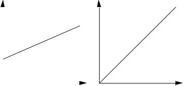
Coding |
35 |
|
|
y2 |
|
|
y2 |
|
|||
|
|
y1 |
|
|
b1 |
||
|
+ |
|
|
|
b0 |
|
|
|
^ = |
|
|
|
y2 |
|
|
|
|
|
|
'1 =y ^ y2
|
|
|
|
y1 |
y'1 = b0 + b1y1 |
|
|
Figure 1.7 |
The regression parameters (b0 and b1) found by regressing y2 |
on y1 (left panel) may be used |
|||||
|
(right panel) to transform y |
1 |
into y' |
such that y' is now on the same scale as y |
2 |
. |
|
|
|
1 |
1 |
|
|
||
2 — Nonlinear transformations
The methods of multidimensional analysis described in this book are often based on covariances or linear correlations. Using them requires that the relationships among variables be made linear by an appropriate transformation. When two variables are not linearly related, their relationship may be described by a secondor higher-degree equation, or by other functional forms, depending on the situation. If the nonlinear form of the equation is derived from ecological theory, as it is often the case in population dynamics models, interpretation of the relationship poses no problem. If, however, a nonlinear transformation is chosen empirically, for reasons of mathematical elegance and without grounding in ecological theory, it may be difficult to find an ecological meaning to it.
The relationship between two variables may be determined with the help of a scatter diagram of the objects in the plane formed by the variables (Fig. 1.8). The principles of analytical geometry may then be used to recognize the type of relationship, which in turn determines the most appropriate type of transformation. A relationship frequently found in ecology is the exponential function, in which a variable y2 increases in geometric progression with respect to y1 , according to one of the following equations:
|
y2 = b ( y1) or y2 = b0b1( y1) or y2 = b0b1( y1 + b2) or else y2 = b0b1( b2 y1) |
(1.3) |
||
Logarithmic |
depending on the number of constants b that shift or amplify the function. Such |
|||
transfor- |
relationships can easily be linearized by using the logarithm of variable y |
2 |
(called y' |
|
mation |
below) instead of y2 itself. The above relationships then become: |
|
2 |
|
|
|
|
||
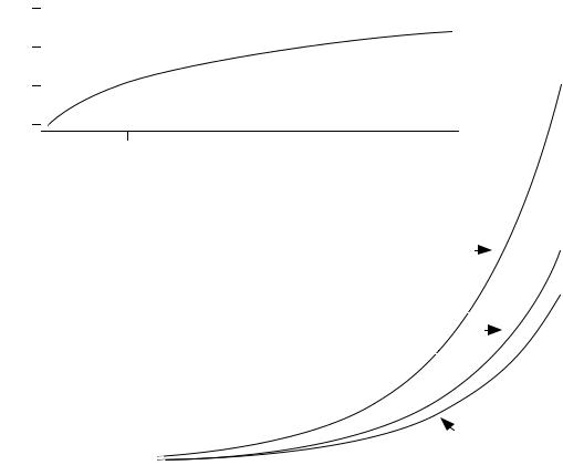
36 |
Complex ecological data sets |
|
|
3
2
y2
1
0
|
|
|
|
|
|
|
110 |
|
|
|
|
|
y2 = loge (y1 + 1) |
|
|
|
|
|
|
|
|
|
|
|
|
|
|
|
|
|||||||||||||||
|
|
|
|
|
|
|
|
|
|
|
|
|
|
|
|
|
|
|
|
|
|
|
|
|
|
|
|
|||||||||||||||||
|
|
|
|
|
|
|
100 |
|
|
|
|
|
|
|
|
|
|
|
|
|
|
|
|
|
|
|
|
|
||||||||||||||||
|
|
|
|
|
|
|
|
|
|
|
|
|
|
|
|
|
|
|
|
|
|
|
|
|
|
|
|
|
|
|
|
|
|
|
|
|
|
|
|
|
|
|||
|
|
|
|
|
|
|
90 |
|
|
|
|
|
|
|
|
|
|
|
|
|
|
|
|
|
|
|
|
|
|
|
|
|
|
|
|
|
|
|
|
|
|
|
||
|
|
|
|
|
|
|
|
|
|
|
|
|
|
|
|
|
|
|
|
|
|
|
|
|
|
|
|
|
|
|
|
|
|
|
|
|
|
|
|
|
|
|||
|
0 |
|
1 |
|
|
2 |
|
|
3 |
|
4 |
|
5 |
|
6 |
|
7 |
|
8 |
|
|
9 |
|
10 |
|
|
|
|
|
|||||||||||||||
|
|
|
|
|
|
|
80 |
|
|
|
|
|
|
|
|
|
|
|
|
|
|
|
|
|
|
|
|
|
|
|
|
|
|
|
|
|
|
|
|
|
|
|
||
|
|
|
|
|
|
|
|
|
|
|
|
|
|
|
|
|
|
|
|
|
|
|
|
|
|
|
|
|
|
|
|
|
|
|
|
|
|
|
|
|
|
|||
|
|
|
|
|
|
|
|
|
|
|
|
|
|
|
|
|
|
|
|
|
|
|
|
|
|
|
|
|
|
|
|
|
|
|
|
|
|
|
|
|
|
|||
|
|
|
|
|
|
|
70 |
|
|
|
|
|
|
|
|
|
|
|
|
|
|
|
|
|
|
|
|
|
|
|
|
|
|
|
|
|
|
|
|
|
|
|
||
|
|
|
|
|
|
|
|
|
|
|
|
|
|
|
|
|
|
|
|
|
|
|
|
|
|
|
|
|
|
|
|
|
|
|
|
|
|
|
|
|
|
|||
|
|
|
|
|
|
|
60 |
|
|
|
|
|
|
|
|
|
|
|
|
|
|
|
|
y2 |
= 0.8 (1.5(y1 + 2)) |
|
|
|||||||||||||||||
|
|
|
|
|
|
|
|
|
|
|
|
|
|
|
|
|
|
|
|
|
|
|
|
|
||||||||||||||||||||
|
|
|
|
|
|
|
|
|
|
|
|
|
|
|
|
|
|
|
|
|
|
|
|
|
|
|
|
|||||||||||||||||
|
|
|
|
|
|
y2 |
50 |
|
|
|
|
|
|
|
|
|
|
|
|
|
|
|
|
|
|
|
|
|
|
|
|
|
|
|
|
|
|
|
|
|
|
|
||
|
|
|
|
|
|
|
|
|
|
|
|
|
|
|
|
|
|
|
|
|
|
|
|
|
|
|
|
|
|
|
|
|
|
|
|
|
|
|
|
|
||||
|
|
|
|
|
|
40 |
|
|
|
|
|
|
|
|
|
|
|
|
|
|
|
|
|
|
|
|
|
|
|
|
|
|
|
|
|
|
|
|
|
|
|
|||
|
|
|
|
|
|
|
|
|
|
|
|
|
|
|
|
|
|
|
|
|
|
|
|
|
|
|
|
|
|
|
y |
= 1.5(y1) |
|
|
|
|
||||||||
|
|
|
|
|
|
|
|
|
|
|
|
|
|
|
|
|
|
|
|
|
|
|
|
|
|
|
|
|
|
|
|
|
|
|
||||||||||
|
|
|
|
|
|
|
|
|
|
|
|
|
|
|
|
|
|
|
|
|
|
|
|
|
|
|
|
|
|
|
|
|
|
|
|
|
|
|||||||
|
|
|
|
|
|
|
30 |
|
|
|
|
|
|
|
|
|
|
|
|
|
|
|
|
|
|
|
|
|
|
|
2 |
|
|
|
|
|
|
|
|
|||||
|
|
|
|
|
|
|
|
|
|
|
|
|
|
|
|
|
|
|
|
|
|
|
|
|
|
|
|
|
|
|
|
|
|
|
|
|
|
|
|
|
|
|||
|
|
|
|
|
|
|
|
|
|
|
|
|
|
|
|
|
|
|
|
|
|
|
|
|
|
|
|
|
|
|
|
|
|
|
|
|
|
|
|
|
|
|||
|
|
|
|
|
|
|
20 |
|
|
|
|
|
|
|
|
|
|
|
|
|
|
|
|
|
|
|
|
|
|
|
|
|
|
|
|
|
|
|
|
|
|
|
||
|
|
|
|
|
|
|
|
|
|
|
|
|
|
|
|
|
|
|
|
|
|
|
|
|
|
|
|
|
|
|
|
|
|
|
|
|
|
|
|
|
|
|||
|
|
|
|
|
|
|
10 |
|
|
|
|
|
|
|
|
|
|
|
|
|
|
|
|
|
|
|
|
|
|
|
|
|
|
|
y2 = 0.8 (1.5(y1)) |
|
|
|||||||
|
|
|
|
|
|
|
|
|
|
|
|
|
|
|
|
|
|
|
|
|
|
|
|
|
|
|
|
|
|
|
|
|
|
|
|
|||||||||
|
|
|
|
|
|
|
0 |
|
|
|
|
|
|
|
|
|
|
|
|
|
|
|
|
|
|
|
|
|
|
|
|
|
|
|
|
|
||||||||
|
|
|
|
|
|
|
|
|
|
|
|
|
|
|
|
|
|
|
|
|
|
|
|
|
|
|
|
|
|
|
|
|
|
|
|
|
|
|
|
|
|
|||
|
|
|
|
|
|
|
|
|
|
|
|
|
|
|
|
|
|
|
|
|
|
|
|
|
|
|
|
|
|
|
|
|
|
|
|
|
|
|
|
|
|
|
|
|
|
|
|
|
|
|
|
|
|
|
0 |
|
|
|
|
|
2 |
|
|
|
|
|
4 |
|
|
|
|
|
|
6 |
|
|
8 |
|
10 |
||||||||||
y1
Figure 1.8 The relationship between variables may often be recognized by plotting them one against the other. In the upper panel, y2 varies as the natural logarithm of y1 . In the lower panel, y2 is an exponential function of y1 . These curves (and corresponding equations) may take different forms, depending on the modifying constants b (eq. 1.3).
y'2 |
= log ( y2) = b'y1 , or |
y'2 |
= |
b'0 + b'1 y1 , |
|
or y'2 = |
b'0 + b'1 ( y1 + b2) , or |
y'2 |
= |
b'0 + b'1b2 y1 |
(1.4) |
where the b's are the logarithms of constants b in eq. 1.3. |
|
||||
If two variables display a logarithmic relationship of the form |
|
||||
|
y2 = logb ( y1) |
|
|
(1.5) |
|
Coding |
37 |
|
|
where b is the base of the logarithm, their relationship can be made linear by applying a log–1 transformation to y2 :
y'2 = b ( y2) = y1 |
(1.6) |
When a nonlinear form may be assumed from knowledge of the ecological process involved, the corresponding equation can be used as the basis for a linearizing transformation. For instance, the nonlinear equation
Nt = N0ert |
(1.7) |
describes the exponential growth of a population, as observed in population explosions. In this equation, the independent variable is time (t); N0 and Nt are the population sizes at times 0 and t, respectively; r is the Malthus parameter describing the intrinsic rate of increase of the population. This nonlinear equation indicates that Nt must be transformed into its natural logarithm. After this transformation, ln(Nt) is linearly related to t: ln(Nt) = ln(N0) + rt.
3 — Combining descriptors
Another transformation which is often used consists in combining different descriptors by addition, subtraction, multiplication or division. In limnology, for example, the ratio (surface O2/ bottom O2) is often used as a descriptor. So is the Pearsall ionic ratio, all ions being in the same physical units:
y = |
---------------------Na + K |
(1.8) |
|
Mg + Ca |
|
Beware, however, of the spurious correlations that may appear when comparing ratio variables to others. Jackson & Somers (1991a) describe the problem and recommend that permutation tests (Section 1.2) be employed with ratios.
It may also be required to take into account a factor of magnitude or size. For example, when observation units are of different sizes, the number of specimens of each species may be divided by the area or the volume of the unit (depending on whether the units come from an area or a volume), or by some other measure of the sampling effort. One must exert care when interpreting the results, however, since large observation units are more representative of populations than small ones.
4 — Ranging and standardization
Quantitative variables, used in ecology as environmental descriptors, are often expressed in incompatible units such as metres, mg L–1, pH units, etc. In order to compare such descriptors, or before using them together in a classification or ordination procedure, they must be brought to some common scale. Among the

38 |
Complex ecological data sets |
|
|
methods available, some only eliminate size differences while others reduce both the size and variability to a common scale.
Translation, a method previously discussed, allows one to centre the data, eliminating size differences due to the position of the zero on the various scales. Centring is done by subtracting the mean of the observations ( y) from each value yi :
y'i = yi – y |
(1.9) |
For relative-scale variables (Subsection 1.4.1), dividing each yi by the largest observed value is a way, based on expansion, to bring all values in the range [0, 1] (Cain & Harrison, 1958):
y'i = yi ⁄ ymax |
(1.10) |
For interval-scale variables, whose range may include negative values, the absolute value of the largest positive or negative value is used as divisor. The transformed values are in the interval [–1, +1].
Other methods allow the simultaneous adjustment of the magnitude and the Ranging variability of the descriptors. The method of ranging, proposed by Sneath & Sokal (1973), reduces the values of a variable to the interval [0, 1] by first subtracting the
minimum observed for each variable and then dividing by the range:
y'i |
= |
y i |
– ymin |
(1.11) |
|
--------------------------y max – ymin |
|||||
|
|
|
|||
Equation 1.10 is the form of ranging (eq. 1.11) to use with relative-scale variables (Subsection 1.4.1) for which ymin is always zero.
The most widely used method for making descriptors compatible is to standardize the data (transformation into so-called “z-scores”). This method will be fully discussed in Section 4.2, dealing with correlation. Principal components (Section 9.2) are
Standardifrequently computed using standardized data. Standardization is achieved by zation subtracting the mean (translation) and dividing by the standard deviation (sy ) of the
variable (expansion):
zi |
yi |
– y |
(1.12) |
= ------------ |
|||
|
|
sy |
|
The position of each object on the transformed variable zi is expressed in standard deviation units; as a consequence, it refers to the group of objects from which sy has been estimated. The new variable zi is called a standardized variable. Such a variable has three interesting properties: its mean is zero (z = 0 ); its variance and hence its standard deviation are 1 (s2z = sz = 1 ); it is also a dimensionless variable (Chapter 3) since the physical dimensions (metres, mg L-1, etc.) in the numerator and denominator cancel out. Transformations 1.6, 1.8 and 1.9 also produce dimensionless variables.
Coding |
39 |
|
|
Beware of the “default options” of computer programs that may implicitly or explicitly suggest to standardize all variables before data analysis. Milligan & Cooper (1988) report simulation results showing that, for clustering purposes, if a transformation is needed, the ranging transformation (eqs. 1.10 and 1.11) gives results that are in general far superior to those obtained using standardization (eq. 1.12).
5 — Implicit transformation in association coefficients
When descriptors with different scales are used together to compare objects, the choice of the association coefficient (Section 7.6) may partly determine the type of transformation that must be applied to the descriptors. Some coefficients give equal weights to all variables independently of their scales while others take into account the magnitude of variation of each one. Since the amount of information (in the sense of information theory; Chapter 6) in a quantitative descriptor increases as a function of its variance, equalizing the variances before the association coefficient is computed is a way to ensure that all descriptors have the same weight. It is for ecologists to decide the kind of contribution they expect from each descriptor; again, beware of the “default options” of computer programs.
Some association coefficients require that the data be expressed as integers. Depending on the capabilities of the computer program and the degree of discrimination required, ecologists may decide to use the closest integer value, or to multiply first all values by 10 or 100, or else to apply some other simple transformation to make the data compatible with the coefficient to be computed.
6 — Normalization
Another type of transformation, called normalizing transformation, is performed on descriptors to make the frequency distributions of their data values look like the normal curve of errors — or, at least, as unskewed as possible. Indeed, several of the methods used in multivariate data analysis have been developed under the assumption that the variables are normally distributed. Although most of these methods do not actually require full normality (i.e. no skewness nor kurtosis), they may perform better if the distributions of values are, at least, not skewed. Skewed distributions, as in Figs. 1.8 and 1.9, are such that the variance of the distribution is controlled mostly by the few points in the extreme right tail; so, variance-partitioning methods such as principal component analysis (Chapter 9) or spectral analysis (Chapter 12) would bring out components expressing the variation of these few data points first instead of the variation of the bulk of data values. Normalizing transformations also have the property of reducing the heteroscedasticity of descriptors (Box 1.4).
The data analysis phase of research should always start by looking at the distributions of values for the different variables, i.e. computing basic distribution statistics (including skewness and kurtosis, eqs. 4.50-4.52), drawing histograms of frequency distributions, and testing for normality (described in Section 4.9). A normalizing transformation may have to be found for each variable separately; in other

40 |
Complex ecological data sets |
|
|
Homoscedasticity |
Box 1.4 |
Homoscedasticity, also called homogeneity or equality of the variances, technically means that the variances of the error terms are equal for all observations. Its antonym is heteroscedasticity or heterogeneity of the variances. Homoscedasticity may actually refer to different properties of the data.
•For a single variable, homoscedasticity of the distribution means that, when the statistical population is sampled repeatedly, the expected value of the variance remains the same, whatever the value of the mean of the data sample. Data drawn from a normal distribution possess this property whereas data drawn from a Poisson distribution, for instance, do not since, in this type of distribution, the variance is equal to the mean.
•In regression analysis, homoscedasticity means that, for all values of the independent variable, the variances of the corresponding values of the dependent variable (called “error variances”) are the same.
•In t-test, analysis of variance and discriminant analysis, homoscedasticity means that variances are equal in all groups, for each variable.
cases, one is looking for the best transformation that would normalize several variables.
• 6.1 — Ecologists often encounter distributions where a species is abundant in a few observation units (quadrats, etc.), fairly abundant in more, present in even more, and absent in many; this is in agreement with the concept of ecological niche briefly explained in Section 1.0, if the sampling programme covers a large enough area or environmental gradient. Distributions of this type are clearly not normal, being strongly skewed to the right (long tail in the higher values). Needless to say, environmental variables may also have non-normal distributions. For instance, the scales on which chemical variables are measured are conventions of chemistry which have no relation whatsoever with the processes generating these values in nature. So, any normalizing transformation is as good as the scale on which these data were originally measured.
Skewed data are often transformed by taking logarithms (below) or square roots. Square root is the least drastic transformation and is used to normalize data that have a Poisson distribution, where the variance is equal to the mean, whereas the logarithmic transformation is applicable to data that depart more widely from a normal distribution (Fig. 1.9). Several intermediate transformations have been proposed between these
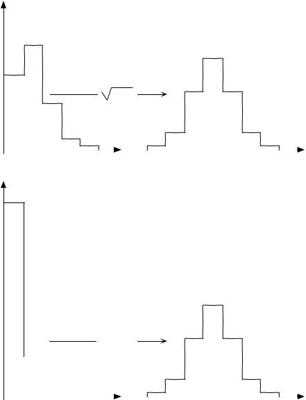
Coding |
41 |
|
|
Frequency
y + c
|
|
|
|
|
|
|
|
|
|
|
|
|
|
0 |
200 |
|
400 |
0 |
10 |
20 |
|||||||
|
|
Raw data |
|
|
|
|
|
Transformed data |
|
|
|||
Frequency
log (y + c)
|
|
|
|
|
|
|
|
|
|
|
|
|
|
|
|
|
|
|
|
|
|
|
|
|
|
|
|
|
|
|
|
|
|
|
|
|
|
|
|
|
|
|
|
|
|
|
|
|
|
|
0 |
|
|
|
|
|
|
|
|
|
|
|
|
|
|
|
|
200 |
|
400 |
0 |
1 |
2 |
3 |
||||||||||
|
|
|
Raw data |
|
|
|
|
|
Transformed data |
|
|
|||||
Figure 1.9 Numerical examples. Upper panel: Data that follow a Poisson distribution (left) can be normalized by the square root transformation (right). For a given species, these frequencies may represent the number of quadrats (ordinate) occupied by the number of specimens shown along the abscissa. Lower panel: Data distribution (left) that can be normalized by a logarithmic transformation (right).
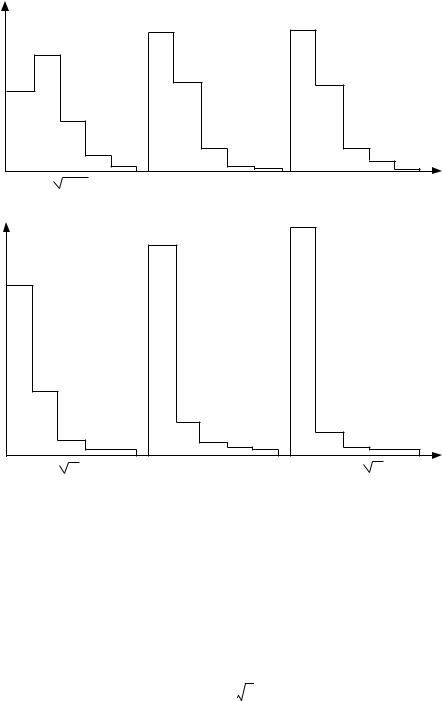
42 |
Complex ecological data sets |
|
|
Frequency
y + c |
log2 ( y + c ) |
log1.5 ( y + c ) |
Frequency
3 y |
log ( y + c ) |
arc sin h y |
Figure 1.10 Numerical examples. Each histogram is labelled by the normalizing transformation to be used in that case.
extremes (Fig. 1.10): cubic root, log2, logp, etc. The hyperbolic transformation is useful for one particular type of data, which share the two extreme types at the same time (when the standard deviation is proportional to the mean, with many observations of a very small size which follow a Poisson distribution: Quenouille, 1950; Barnes, 1952). The angular or arcsine transformation is appropriate for percentages and proportions (Sokal & Rohlf, 1981, 1995):
y'i = arcsin yi |
(1.13) |
Coding |
43 |
|
|
In case of doubt, one may try several of these transformations and perform a test of normality (Section 4.7), or compute the skewness of the transformed data, retaining the transformation that produces the most desirable results. Alternatively, the Box-Cox method (point 6.2, below) may be used to find the best normalizing transformation.
A logarithmic transformation is computed as follows:
Logarithmic |
|
|
= log (b0 + b1 yi) |
|
|
|
transfor- |
|
y'i |
|
|
(1.14) |
|
mation |
The base of logarithm chosen has no influence on the normalising power, since |
|||||
|
||||||
|
transformation from one base to another is a linear change of scale (expansion, see 1 |
|||||
|
above: logd yi |
= logc yi ⁄ logcd ). When the data to be transformed are all strictly |
||||
|
positive (all yi |
> 0), it is not necessary to carry out a translation (b0 |
= 0). When the |
|||
|
data contain fractional values between 0 and 1, one may multiply all values by some |
|||||
|
appropriate constant in order to avoid negative transformed values: y'i |
= log (b1 yi) . |
||||
|
When the data to be transformed contain negative or null values, a translation must be |
|||||
|
applied first, y'i |
= log (b0 + yi) , since the logarithmic function is defined over the set |
||||
|
of positive real numbers only. One should choose for translation a constant b0 which is |
|||||
|
of the same order of magnitude as the significant digits of the variable to be |
|||||
|
transformed; for example, b0 = 0.01 for data between 0.00 and 0.09 (the same purpose |
|||||
|
would have been achieved by selecting b0 = 1 and b1 |
= 100). For species abundance |
||||
|
data, this rule produces the classical transformation y'i |
= log ( yi + 1) . |
||||
|
• 6.2 — When there is no a priori reason for selecting one or the other of the above |
|||||
Box-Cox |
transformations, the Box-Cox method allows one to empirically estimate what is the |
|||||
method |
most appropriate exponent of the following general transformation function: |
|||||
|
|
y' = |
( yγ – 1) ⁄ γ |
(for γ ≠ 0) |
(1.15) |
|
|
|
i |
i |
|
|
|
|
and |
y'i |
= ln ( yi) |
(for γ = 0) |
|
|
As before, y'i is the transformed value of observation yi . In this transformation, the value γ is used that maximizes the following log likelihood function:
L = – (ν ⁄ 2) ln (s2y') + (γ – 1) (ν ⁄ n) ∑ln ( yi) |
(1.16) |
i |
|
since it is this value which yields the best transformation to normality (Box & Cox, 1964; Sokal & Rohlf, 1995). The value L that maximizes this likelihood function is found by iterative search. In this equation, s2y' is the variance of the transformed values y'i . When analysing several groups of observations at the same time (below), s2y' is estimated instead by the within-group, or residual variance computed in a one-way ANOVA. The group size is n and ν is the number of degrees of freedom (ν = n – 1 if the computation is made for a single group). All yi values must be strictly positive numbers since logarithms are taken in the likelihood function L (eq. 1.16); all values
44 |
Complex ecological data sets |
|
|
may easily be made strictly positive by translation, as discussed in Subsection 1 above. It is interesting to note that, if γ = 1, the function is a simple linear transformation; if γ = 1/2, the function becomes the square root transformation; when γ = 0, the transformation is logarithmic; γ = –1 yields the reciprocal transformation.
Readers are invited to take a value (say 150) and transform it, using eq. 1.15, with a variety of values of γ gradually tending toward 0 (say 1, 0.1, 0.01, 0.001, etc.). Comparing the results to the logarithmic transformation will make it obvious that this transformation is indeed the limit of eq. 1.15 when γ tends towards 0.
Another log likelihood function L' is proposed by Sokal & Rohlf (1995) in order to achieve homogeneity of the variances for several groups of observations of a given variable, together with the normality of their distributions. This generalized Box-Cox transformation may also be applied to the identification of the best normalizing transformation for several species, for a given set of sampling sites.
|
• 6.3 — When the data distribution includes several groups, or when the same |
||
|
transformation is to be applied to several quantitative and dimensionally homogeneous |
||
Taylor’s |
descriptors (Chapter 3; for instance, a species abundance data table), Taylor’s (1961) |
||
power law |
power law provides the basis for another general transformation which stabilizes the |
||
|
variances and thus makes the data more likely to conform to the assumptions of |
||
|
parametric analysis, including normality (Southwood, 1966; see also Downing, 1979 |
||
|
on this subject). This law relates the means and variances of the k groups through |
||
|
equation |
|
|
|
s2y |
= a ( yk) b |
(1.17) |
|
|
k |
|
from which constants a and b can be computed by nonlinear regression. When the latter is not available, an approximation of b may be calculated by linear regression of the logarithmic form
|
log s2y |
= log a + b log yk |
(1.18) |
|||||
|
|
|
k |
|
|
|
|
|
Having found the value of b, the variance stabilizing transformations |
|
|||||||
|
|
|
|
|
b |
|
|
|
|
|
|
|
|
1 – -- |
|
|
|
|
y'i |
= |
2 |
(for b ≠ 2) |
|
|||
|
yi |
|
|
(1.19) |
||||
or |
y'i |
= |
ln(yi) |
(for b = 2) |
|
|||
are applied to the data. |
|
|
|
|
|
|
|
|
Omnibus • 6.4 — The following method represents an omnibus normalizing procedure that procedure should be able to normalize most kinds of data. The procedure is easy to carry out using most standard statistical packages running on microcomputers. The package
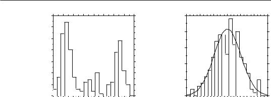
|
|
|
|
|
|
Coding |
|
|
|
|
|
|
|
45 |
|
35 |
|
|
|
|
|
|
25 |
|
|
|
|
|
|
|
30 |
|
|
|
|
|
|
20 |
|
|
|
|
|
|
|
|
|
|
|
|
|
|
|
|
|
|
|
|
|
|
25 |
|
|
|
|
|
|
|
|
|
|
|
|
|
Frequency |
20 |
|
|
|
|
|
Frequency |
15 |
|
|
|
|
|
|
|
|
|
|
|
|
|
|
|
|
|
||||
15 |
|
|
|
|
|
|
|
|
|
|
|
|||
|
|
|
|
|
10 |
|
|
|
|
|
|
|||
|
|
|
|
|
|
|
|
|
|
|
|
|||
|
|
|
|
|
|
|
|
|
|
|
|
|
|
|
|
10 |
|
|
|
|
|
|
|
|
|
|
|
|
|
|
5 |
|
|
|
|
|
|
5 |
|
|
|
|
|
|
|
|
|
|
|
|
|
|
|
|
|
|
|
|
|
|
0 |
|
|
|
|
|
|
0 |
|
|
|
|
|
|
|
0 |
2 |
4 |
6 |
8 |
10 12 14 16 |
|
-3 |
-2 |
-1 |
0 |
1 |
2 |
3 |
|
|
|
|
|
Raw data |
|
|
|
Normalized data |
|
|
|||
Figure 1.11 The omnibus procedure has been used to normalize a set of 200 data values with tri-modal distribution (left). A normal curve has been fitted to the transformed data (right).
must have a pseudo-random number generator for random normal deviates, i.e. values drawn at random from a normal distribution.
(1) Write the quantitative or semiquantitative descriptor to be normalized into a data base. Sort the data base in increasing values for that descriptor. (2) Create a new descriptor with the same number of values, using a pseudo-random normal deviate generator. Write it into another data base and sort it also in order of increasing values.
(3)Copy the sorted normal deviate values into the sorted data base containing the descriptor to be normalized. Sort the data base back into the original order if necessary.
(4)Use the normal deviates as a monotonic proxy for the original descriptor. Figure 1.11 shows an example of this transformation.
This procedure may be modified to handle ex aequo (tied) values (Section 5.3). Tied values may either receive the same normal deviate value, or they may be sorted in some random order and given neighbouring normal deviate values; one should select a solution that makes sense considering the data at hand.
Powerful as it is, this transformation only makes sense for data that have no more than ordinal value in the analysis to be conducted. The transformed data may be used in methods of data analysis that perform better in the presence of normality of the distributions. Several such methods will be studied in chapters 9 and 11. The main disadvantage is that a back-transformation is difficult. If the study requires that values of this descriptor be forecasted by a model, the data base itself will have to be used to find the original descriptor values which are the closest to the forecasted normal deviate. An interpolation may have to be made between these values.
46 |
Complex ecological data sets |
|
|
7 — Dummy variable (binary) coding
Multistate qualitative descriptors may be binary-coded as dummy variables. This coding is interesting because it allows the use of qualitative descriptors in procedures such as multiple regression, discriminant analysis or canonical analysis, that have been developed for quantitative variables and in which binary variables may also be used. A multistate qualitative descriptor with s states is decomposed into (s – 1) dummy variables. An example is the following four-state descriptor:
States |
|
Dummy variables |
|
|
|
|
|
|
|
1 |
1 |
0 |
0 |
0 |
2 |
0 |
1 |
0 |
0 |
3 |
0 |
0 |
1 |
0 |
4 |
0 |
0 |
0 |
1 |
|
|
|
|
|
In this example, three dummy variables are sufficient to binary-code the four states of the original nominal descriptor. Had a fourth dummy variable been included (shaded column above), its information would have been totally linearly dependent (Box 1.1 and Section 2.7) on the first three variables. In other words, the first three dummy variables are enough to determine the states of the multistate qualitative descriptor. Actually, any one of the four dummy variables may be eliminated to return to the condition of linear independence among the remaining ones.
Using this table, the objects are coded, in this example, by three dummy variables instead of a single 4-state descriptor. An object with state 1, for instance, would be
|
recoded [1 0 0], an object with state 2, [0 1 0], and so on. |
|
Other forms of binary coding have been developed for special types of variables. In |
|
phylogenetic analysis, the states of multistate characters are sometimes related by a |
|
hypothesized transformation series, going from the single hypothesized ancestral state |
|
to all the advanced states; such a series can be represented by a directed network where |
|
the states are connected by arrows representing evolutionary progression. A |
|
transformation series may be coded into binary variables using a method proposed by |
|
Kluge & Farris (1969). This same method may be applied to code the spatial |
|
relationships among localities on any geographic network. An example in freshwater |
|
ecology is a group of lakes connected by a river network (Fig. 1.12). |
River |
In this example, a picture made of rivers and lakes is drawn to represent the |
network |
network. A number is assigned to each river segment (which are the edges of the |
|
connected graph), while nodes represent the furcation points. In Fig. 1.12, the coding |
|
is based on the river segments; it could just as well be based on the nodes, if one felt |
|
that the nodes are the important carriers of geographic information (as in Magnan et |
|
al., 1994). If the phenomenon to be modelled is, for example, fish dispersal from |
|
downstream, the arrows can be drawn going upstream, as in Fig. 1.12. In the lake-by- |
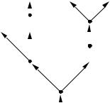
|
|
|
|
|
|
|
|
|
|
|
|
|
|
Missing data |
|
|
|
|
|
|
|
47 |
|||
|
|
|
|
|
|
|
|
|
|
|
|
|
|
|
|
|
|
|
|
|
|
|
|
|
|
|
|
|
|
|
|
|
|
|
|
|
|
|
|
|
|
|
|
|
|
|
|
|
|||
|
|
|
Lake 1 |
|
|
|
Lake 4 |
|
|
Lake 5 |
|
|
|
|
|
|
|
|
|
|
|
|
|||
|
|
|
|
|
|
|
|
|
|
|
|
|
|
|
|
|
|
|
|
Arrows |
|
|
|
|
|
|
Arrow 4 |
|
|
Arrow 5 |
Arrow 6 |
|
|
|
|
|
|
|
|
||||||||||||
|
|
|
|
|
|
|
|
|
|
|
|||||||||||||||
|
|
|
|
|
|
|
|
|
|
|
|
|
|||||||||||||
|
|
|
|
|
|
|
1 |
2 |
3 |
4 |
5 |
6 |
7 |
8 |
|
||||||||||
|
Lake 3 |
|
Lake 2 |
|
|
|
|
|
|
|
|
|
|
|
|
|
|||||||||
|
|
|
|
|
|
|
|
|
|
|
|
|
|
|
|
|
|
|
|
|
|
|
|
|
|
|
|
|
|
|
|
|
|
|
|
|
|
|
|
|
|
|
|
|
|
|
|
|
|
|
|
|
|
|
|
|
|
|
|
|
|
|
Arrow 7 |
|
|
|
|
|
|
|
|
|
|
||||
|
Arrow 2 |
|
Arrow 3 |
|
|
|
|
|
|
|
|
|
Lake 1 |
|
1 |
0 |
1 |
1 |
0 |
0 |
0 |
0 |
|
||
|
|
|
|
|
|
|
|
|
|||||||||||||||||
|
|
|
|
|
Lake 6 |
|
|
Lake 2 |
|
1 |
0 |
1 |
0 |
0 |
0 |
0 |
0 |
|
|||||||
|
|
|
|
|
|
|
|
|
|
|
|
|
|||||||||||||
|
|
|
|
|
|
|
|
|
|
|
|
|
|
|
Lake 3 |
|
1 |
1 |
0 |
0 |
0 |
0 |
0 |
0 |
|
|
|
|
|
|
|
|
|
|
|
|
|
|
|
|
|
|
|||||||||
|
|
|
Arrow 1 |
|
|
|
Arrow 8 |
|
|
Lake 4 |
|
0 |
0 |
0 |
0 |
1 |
0 |
1 |
1 |
|
|||||
|
|
|
|
|
|
|
|
Lake 5 |
|
0 |
0 |
0 |
0 |
0 |
1 |
1 |
1 |
|
|||||||
|
|
|
|
|
|
|
|
|
|
|
|
|
|
|
|
|
|||||||||
|
|
|
|
|
|
|
|
|
|
|
|
|
|
|
Lake 6 |
|
0 |
0 |
0 |
0 |
0 |
0 |
0 |
1 |
|
|
|
|
|
Arrow 0 |
|
|
|
|
|
|
|
|
|
|
|
|
|
|
|
|
|
|
|||
|
|
|
|
|
|
|
|
|
|
|
|
|
|
|
|
|
|
|
|
|
|
||||
|
|
|
|
|
|
|
|
|
|
|
|
|
|
|
|
|
|
|
|
|
|
|
|
|
|
Figure 1.12 Lakes interconnected by a river network (left) can be binary-coded as shown on the right. Numbers are assigned in an arbitrary order to the edges (arrows) of the network. There is no use in representing the “root” of the network (arrow 0); all lakes would be coded ‘1’ for that arrow.
arrow matrix, a value ‘1’ is assigned to each arrow found downstream from the lake, meaning that the corresponding river segment is available for fish to reach that lake. All other arrows are coded ‘0’ for the lake. The resulting matrix is a complete numerical coding of the hydrographic network information: knowing the coding procedure, one could reconstruct the picture from the matrix entries.
The coding method may be tailored to the ecological problem at hand. For a dispersion phenomenon going downstream, arrows could point the other way around; in this case, a lake would be coded ‘1’ in the table for arrows arriving in that lake from upstream. The pattern of interconnections does not even need to be a tree-like structure; it may form a more general type of directed network, but note that no cycle is allowed. Coding the information allows the use of this type of geographical information in different types of numerical models, like multiple regression (Chapter 10) or canonical analysis (Chapter 11). In many of these methods, zeros and ones are interchangeable.
1.6 Missing data
Ecological data matrices are often plagued by missing data. They do not necessarily result from negligence on the part of the field team; most often, they are caused by the breakdown of measuring equipment during field surveys, weather events that prevent sampling sites from being visited on a given date, lost or incorrectly preserved specimens, improper sampling procedures, and so on.
48 |
Complex ecological data sets |
|
|
Three families of solutions are available to cope with this problem for the analysis of field survey data, if one can make the assumption that the missing values occur at random in the data set. Most of the approaches mentioned below are discussed by Little & Rubin (1987), who also propose methods for estimating missing values in controlled experiments (when the missing values are only found in the outcome variable; their Chapter 2) as well as valid model-based likelihood estimation of missing values for situations where the distribution of missing values does not meet the randomness assumption stated above.
Missing values may be represented in data matrices by numbers that do not correspond to possible data values. Codes such as –1 or –9 are often used when the real data in the table are all positive numbers, as it is the case with species abundance data; otherwise, –99 or –999, or other such unambiguous codes, may be used. In spreadsheets, missing values are represented by bullets or other such symbols.
1 — Deleting rows or columns
Delete any row or column of the data matrix (Section 2.1) containing missing values. If a few rows contain most of the missing values, proceed by rowwise (also called listwise) deletion; conversely, if most missing values are found in a few variables only, proceed by columnwise deletion. This is the simplest, yet the most costly method, as it throws away the valuable information present in the remainder of these rows or columns.
2 — Accommodating algorithms to missing data
Accommodate the numerical method in such a way that the missing values are skipped during calculations. For instance, when computing resemblance coefficients among rows (Q-mode; Chapter 7) or columns (R-mode) of the data matrix, a simple method is pairwise deletion of missing values. This means, for example, that when computing a correlation coefficient between variables y1 and y2, if the value of the tenth object is missing for y2, object x10 is skipped in the computation of this correlation value. When it comes to comparing y1 and y3, if x10 has no missing data for these variables, it is then kept in the calculation for this pair of variables. However, one must be aware that covariance and correlation matrices computed in this way may be indefinite (i.e. they may have negative eigenvalues; Table 2.2). Wishart (1978, 1985) lists several such methods developed in the cluster analysis framework, that are used in the CLUSTAN clustering package.
3 — Estimating missing values
Estimate the missing values (called imputation by Little & Rubin, 1987). This is the best strategy when missing values are located all over the data matrix — contrary to the situation where the missing values are found in a few rows or columns only, in which case deletion of these rows or columns may be the strategy of choice. The
Missing data |
49 |
|
|
assumption one has to make when estimating missing values is that the missing data are not grossly atypical compared to those present in the data set. Methods for estimating missing data are interesting in cases where the numerical algorithm required for analysing the data set cannot accommodate missing values. Ecologists should never imagine, however, that the estimated values are ecologically meaningful; as a consequence, they should refrain from attempting to interpret these numbers in ecological terms. Ecologists should also keep in mind that the estimation procedure has not created the missing degrees of freedom that would have accompanied observations carried out in nature or in the laboratory.
Three groups of methods are available for filling in missing values for quantitative data.
•3.1 — The easiest way, which is often used in computer programs, is to replace missing values by the mean of the variable, estimated from the values present in the data table. When doing so, one assumes that nothing is known about the data, outside of the weak assumption mentioned above that the missing value comes from the same population as the non-missing data. Although this solution produces covariance and correlation matrices that are positive semidefinite (Section 2.10), the variances and covariances are systematically underestimated. One way around this problem is to select missing value estimates at random from some distribution with appropriate mean and variance. This is not recommended, however, when the relative positions of the objects are of interest (principal component analysis; Section 9.1). A variant of the same method is to use the median instead of the mean; it is more robust in the sense that it does not assume the distribution of values to be unskewed. It is also applicable to semiquantitative descriptors. For qualitative descriptors, use the most frequent state instead of the mean or median.
•3.2 — Estimate the missing values by regression. Multiple linear regression (Section 10.3), with rowwise deletion of missing values, may be used when there are only a few missing values to estimate. The dependent (response) variable of the regression is the descriptor with missing value(s) while the independent (explanatory) variables are the other descriptors in the data table. After the regression equation has been computed from the objects without missing data, it can be used to estimate the missing value(s). Using this procedure, one assumes the descriptor with missing values to be linearly related to the other descriptors in the data table (unless some form of nonparametric or nonlinear multiple regression is being used) and the data to be approximately multivariate normal. This method also leads to underestimating the variances and covariances, but less so than in 3.1. An alternative approach is to use a regression program allowing for pairwise deletion of missing values in the estimation of the regression coefficients, although, in that case, a maximum likelihood estimation of the covariance matrix would be preferable (Little & Rubin, 1987, p. 152 et seq.).
If such a method cannot be used for estimating the covariance matrix and if the missing values are scattered throughout the data table, an approximate solution may be obtained as follows. Compute a series of simple linear regressions with pairwise
50 |
Complex ecological data sets |
|
|
deletion of missing values, and estimate the missing value from each of these simple regression equations in turn. The mean of these estimates is taken as the working estimated value. The assumptions are basically the same as in the multiple regression case (above).
To estimate missing values in qualitative (nominal) descriptors, use logistic regression (Section 10.3) instead of linear regression.
• 3.3 — Interpolate missing values in autocorrelated data. Positive autocorrelation (Section 1.1) means that near points in time or space are similar. This property allows the interpolation of missing or otherwise unknown values from the values of near points in the series. With spatial data, interpolation is the first step of any mapping procedure, and it may be done in a variety of ways (Subsection 13.2.2), including the kriging method developed by geostatisticians. The simplest such method is to assign to a missing data the value of its nearest neighbour. In time series, interpolation of missing values may be performed using the same methods; see also Shumway & Stoffer, 1982, as well as Mendelssohn & Cury, 1987, for a maximum likelihood method for estimating missing data in a time series using a state-space model.
Myers (1982, 1983, 1984) has proposed a method, called co-kriging, that combines the power of principal component analysis (Section 9.1) with that of kriging. It allows the estimation of unknown values of a data series using both the values of the same variable at neighbouring sites and the known values of other variables, correlated with the first one, observed at the same or neighbouring points in space; the spatial interrelationships of these variables are measured by a cross-variogram. This method should become very important in the future, for estimating missing data in broad-scale ecological surveys and to compute values at unobserved sites on a geographic surface.