Wooldridge_-_Introductory_Econometrics_2nd_Ed

Chapter 2 The Simple Regression Model

In the voting outcome equation in (2.28), R2 0.505. Thus, the share of campaign expenditures explains just over 50 percent of the variation in the election outcomes for this sample. This is a fairly sizable portion.

2.4 UNITS OF MEASUREMENT AND FUNCTIONAL FORM

Two important issues in applied economics are (1) understanding how changing the units of measurement of the dependent and/or independent variables affects OLS estimates and (2) knowing how to incorporate popular functional forms used in economics into regression analysis. The mathematics needed for a full understanding of functional form issues is reviewed in Appendix A.

The Effects of Changing Units of Measurement on OLS Statistics

In Example 2.3, we chose to measure annual salary in thousands of dollars, and the return on equity was measured as a percent (rather than as a decimal). It is crucial to know how salary and roe are measured in this example in order to make sense of the estimates in equation (2.39).

We must also know that OLS estimates change in entirely expected ways when the units of measurement of the dependent and independent variables change. In Example 2.3, suppose that, rather than measuring salary in thousands of dollars, we measure it in dollars. Let salardol be salary in dollars (salardol 845,761 would be interpreted as $845,761.). Of course, salardol has a simple relationship to the salary measured in thousands of dollars: salardol 1,000 salary. We do not need to actually run the regression of salardol on roe to know that the estimated equation is:

We obtain the intercept and slope in (2.40) simply by multiplying the intercept and the slope in (2.39) by 1,000. This gives equations (2.39) and (2.40) the same interpretation. Looking at (2.40), if roe 0, then salaˆrdol 963,191, so the predicted salary is $963,191 [the same value we obtained from equation (2.39)]. Furthermore, if roe increases by one, then the predicted salary increases by $18,501; again, this is what we concluded from our earlier analysis of equation (2.39).

Generally, it is easy to figure out what happens to the intercept and slope estimates when the dependent variable changes units of measurement. If the dependent variable is multiplied by the constant c—which means each value in the sample is multiplied by c—then the OLS intercept and slope estimates are also multiplied by c. (This assumes nothing has changed about the independent variable.) In the CEO salary example, c 1,000 in moving from salary to salardol.

41

We can also use the CEO salary example to see what happens when we change the units of measurement of the independent variable. Define roedec roe/100

Q U E S T I O N 2 . 4 to be the decimal equivalent of roe; thus, roedec 0.23 means a return on equity of 23 percent. To focus on changing the units of measurement of the independent variable, we return to our original dependent

variable, salary, which is measured in thousands of dollars. When we regress salary on roedec, we obtain

The coefficient on roedec is 100 times the coefficient on roe in (2.39). This is as it should be. Changing roe by one percentage point is equivalent to roedec 0.01. From (2.41), if roedec 0.01, then salˆary 1850.1(0.01) 18.501, which is what is obtained by using (2.39). Note that, in moving from (2.39) to (2.41), the independent variable was divided by 100, and so the OLS slope estimate was multiplied by 100, preserving the interpretation of the equation. Generally, if the independent variable is divided or multiplied by some nonzero constant, c, then the OLS slope coefficient is also multiplied or divided by c respectively.

The intercept has not changed in (2.41) because roedec 0 still corresponds to a zero return on equity. In general, changing the units of measurement of only the independent variable does not affect the intercept.

In the previous section, we defined R-squared as a goodness-of-fit measure for OLS regression. We can also ask what happens to R2 when the unit of measurement of either the independent or the dependent variable changes. Without doing any algebra, we should know the result: the goodness-of-fit of the model should not depend on the units of measurement of our variables. For example, the amount of variation in salary, explained by the return on equity, should not depend on whether salary is measured in dollars or in thousands of dollars or on whether return on equity is a percent or a decimal. This intuition can be verified mathematically: using the definition of R2, it can be shown that R2 is, in fact, invariant to changes in the units of y or x.

Incorporating Nonlinearities in Simple Regression

So far we have focused on linear relationships between the dependent and independent variables. As we mentioned in Chapter 1, linear relationships are not nearly general enough for all economic applications. Fortunately, it is rather easy to incorporate many nonlinearities into simple regression analysis by appropriately defining the dependent and independent variables. Here we will cover two possibilities that often appear in applied work.

In reading applied work in the social sciences, you will often encounter regression equations where the dependent variable appears in logarithmic form. Why is this done? Recall the wage-education example, where we regressed hourly wage on years of education. We obtained a slope estimate of 0.54 [see equation (2.27)], which means that each additional year of education is predicted to increase hourly wage by 54 cents.

42

Because of the linear nature of (2.27), 54 cents is the increase for either the first year of education or the twentieth year; this may not be reasonable.

Suppose, instead, that the percentage increase in wage is the same given one more year of education. Model (2.27) does not imply a constant percentage increase: the percentage increases depends on the initial wage. A model that gives (approximately) a constant percentage effect is

where log( ) denotes the natural logarithm. (See Appendix A for a review of logarithms.) In particular, if u 0, then

Notice how we multiply 1 by 100 to get the percentage change in wage given one additional year of education. Since the percentage change in wage is the same for each additional year of education, the change in wage for an extra year of education increases as education increases; in other words, (2.42) implies an increasing return to education. By exponentiating (2.42), we can write wage exp( 0 1educ u). This equation is graphed in Figure 2.6, with u 0.

F i g u r e 2 . 6

wage exp( 0 1educ), with 1 0.

wage

43

Estimating a model such as (2.42) is straightforward when using simple regression. Just define the dependent variable, y, to be y log(wage). The independent variable is represented by x educ. The mechanics of OLS are the same as before: the intercept and slope estimates are given by the formulas (2.17) and (2.19). In other words, we obtain ˆ0 and ˆ1 from the OLS regression of log(wage) on educ.

E X A M P L E 2 . 1 0

( A L o g W a g e E q u a t i o n )

Using the same data as in Example 2.4, but using log(wage) as the dependent variable, we obtain the following relationship:

n 526, R2 0.186.

The coefficient on educ has a percentage interpretation when it is multiplied by 100: wage increases by 8.3 percent for every additional year of education. This is what economists mean when they refer to the “return to another year of education.”

It is important to remember that the main reason for using the log of wage in (2.42) is to impose a constant percentage effect of education on wage. Once equation (2.42) is obtained, the natural log of wage is rarely mentioned. In particular, it is not correct to say that another year of education increases log(wage) by 8.3%.

The intercept in (2.42) is not very meaningful, as it gives the predicted log(wage), when educ 0. The R-squared shows that educ explains about 18.6 percent of the variation in log(wage) (not wage). Finally, equation (2.44) might not capture all of the nonlinearity in the relationship between wage and schooling. If there are “diploma effects,” then the twelfth year of education—graduation from high school— could be worth much more than the eleventh year. We will learn how to allow for this kind of nonlinearity in Chapter 7.

Another important use of the natural log is in obtaining a constant elasticity model.

E X A M P L E 2 . 1 1

( C E O S a l a r y a n d F i r m S a l e s )

We can estimate a constant elasticity model relating CEO salary to firm sales. The data set is the same one used in Example 2.3, except we now relate salary to sales. Let sales be annual firm sales, measured in millions of dollars. A constant elasticity model is

where 1 is the elasticity of salary with respect to sales. This model falls under the simple regression model by defining the dependent variable to be y log(salary) and the independent variable to be x log(sales). Estimating this equation by OLS gives

44

Chapter 2 The Simple Regression Model

n 209, R2 0.211.

The coefficient of log(sales) is the estimated elasticity of salary with respect to sales. It implies that a 1 percent increase in firm sales increases CEO salary by about 0.257 per- cent—the usual interpretation of an elasticity.

The two functional forms covered in this section will often arise in the remainder of this text. We have covered models containing natural logarithms here because they appear so frequently in applied work. The interpretation of such models will not be much different in the multiple regression case.

It is also useful to note what happens to the intercept and slope estimates if we change the units of measurement of the dependent variable when it appears in logarithmic form. Because the change to logarithmic form approximates a proportionate change, it makes sense that nothing happens to the slope. We can see this by writing the rescaled variable as c1yi for each observation i. The original equation is log(yi) 0 1xi ui. If

we add log(c1) to both sides, we get log(c1) log(yi) [log(c1) 0] 1xi ui, or log(c1yi) [log(c1) 0] 1xi ui. (Remember that the sum of the logs is equal to

the log of their product as shown in Appendix A.) Therefore, the slope is still 1, but the intercept is now log(c1) 0. Similarly, if the independent variable is log(x), and we change the units of measurement of x before taking the log, the slope remains the same but the intercept does not change. You will be asked to verify these claims in Problem 2.9.

We end this subsection by summarizing four combinations of functional forms available from using either the original variable or its natural log. In Table 2.3, x and y stand for the variables in their original form. The model with y as the dependent variable and x as the independent variable is called the level-level model, because each variable appears in its level form. The model with log(y) as the dependent variable and x as the independent variable is called the log-level model. We will not explicitly discuss the level-log model here, because it arises less often in practice. In any case, we will see examples of this model in later chapters.

Table 2.3

Summary of Functional Forms Involving Logarithms

45

The last column in Table 2.3 gives the interpretation of 1. In the log-level model, 100 1 is sometimes called the semi-elasticity of y with respect to x. As we mentioned in Example 2.11, in the log-log model, 1 is the elasticity of y with respect to x. Table 2.3 warrants careful study, as we will refer to it often in the remainder of the text.

The Meaning of “Linear” Regression

The simple regression model that we have studied in this chapter is also called the simple linear regression model. Yet, as we have just seen, the general model also allows for certain nonlinear relationships. So what does “linear” mean here? You can see by looking at equation (2.1) that y 0 1x u. The key is that this equation is linear in the parameters, 0 and 1. There are no restrictions on how y and x relate to the original explained and explanatory variables of interest. As we saw in Examples 2.7 and 2.8, y and x can be natural logs of variables, and this is quite common in applications. But we need not stop there. For example, nothing prevents us from using simple regression to

—

estimate a model such as cons 0 1 inc u, where cons is annual consumption and inc is annual income.

While the mechanics of simple regression do not depend on how y and x are defined, the interpretation of the coefficients does depend on their definitions. For successful empirical work, it is much more important to become proficient at interpreting coefficients than to become efficient at computing formulas such as (2.19). We will get much more practice with interpreting the estimates in OLS regression lines when we study multiple regression.

There are plenty of models that cannot be cast as a linear regression model because they are not linear in their parameters; an example is cons 1/( 0 1inc) u. Estimation of such models takes us into the realm of the nonlinear regression model, which is beyond the scope of this text. For most applications, choosing a model that can be put into the linear regression framework is sufficient.

2.5 EXPECTED VALUES AND VARIANCES OF THE OLS ESTIMATORS

In Section 2.1, we defined the population model y 0 1x u, and we claimed that the key assumption for simple regression analysis to be useful is that the expected value of u given any value of x is zero. In Sections 2.2, 2.3, and 2.4, we discussed the algebraic properties of OLS estimation. We now return to the population model and study the statistical properties of OLS. In other words, we now view ˆ0 and ˆ1 as estimators for the parameters 0 and 1 that appear in the population model. This means that we will study properties of the distributions of ˆ0 and ˆ1 over different random samples from the population. (Appendix C contains definitions of estimators and reviews some of their important properties.)

Unbiasedness of OLS

We begin by establishing the unbiasedness of OLS under a simple set of assumptions. For future reference, it is useful to number these assumptions using the prefix “SLR” for simple linear regression. The first assumption defines the population model.

46

Chapter 2 The Simple Regression Model

A S S U M P T I O N S L R . 1 ( L I N E A R I N P A R A M E T E R S )

In the population model, the dependent variable y is related to the independent variable x and the error (or disturbance) u as

where 0 and 1 are the population intercept and slope parameters, respectively.

To be realistic, y, x, and u are all viewed as random variables in stating the population model. We discussed the interpretation of this model at some length in Section 2.1 and gave several examples. In the previous section, we learned that equation (2.47) is not as restrictive as it initially seems; by choosing y and x appropriately, we can obtain interesting nonlinear relationships (such as constant elasticity models).

We are interested in using data on y and x to estimate the parameters 0 and, especially, 1. We assume that our data were obtained as a random sample. (See Appendix C for a review of random sampling.)

A S S U M P T I O N S L R . 2 ( R A N D O M S A M P L I N G )

We can use a random sample of size n, {(xi,yi): i 1,2,…,n}, from the population model.

We will have to address failure of the random sampling assumption in later chapters that deal with time series analysis and sample selection problems. Not all cross-sectional samples can be viewed as outcomes of random samples, but many can be.

We can write (2.47) in terms of the random sample as

where ui is the error or disturbance for observation i (for example, person i, firm i, city i, etc.). Thus, ui contains the unobservables for observation i which affect yi. The ui should not be confused with the residuals, uˆi, that we defined in Section 2.3. Later on, we will explore the relationship between the errors and the residuals. For interpreting 0 and 1 in a particular application, (2.47) is most informative, but (2.48) is also needed for some of the statistical derivations.

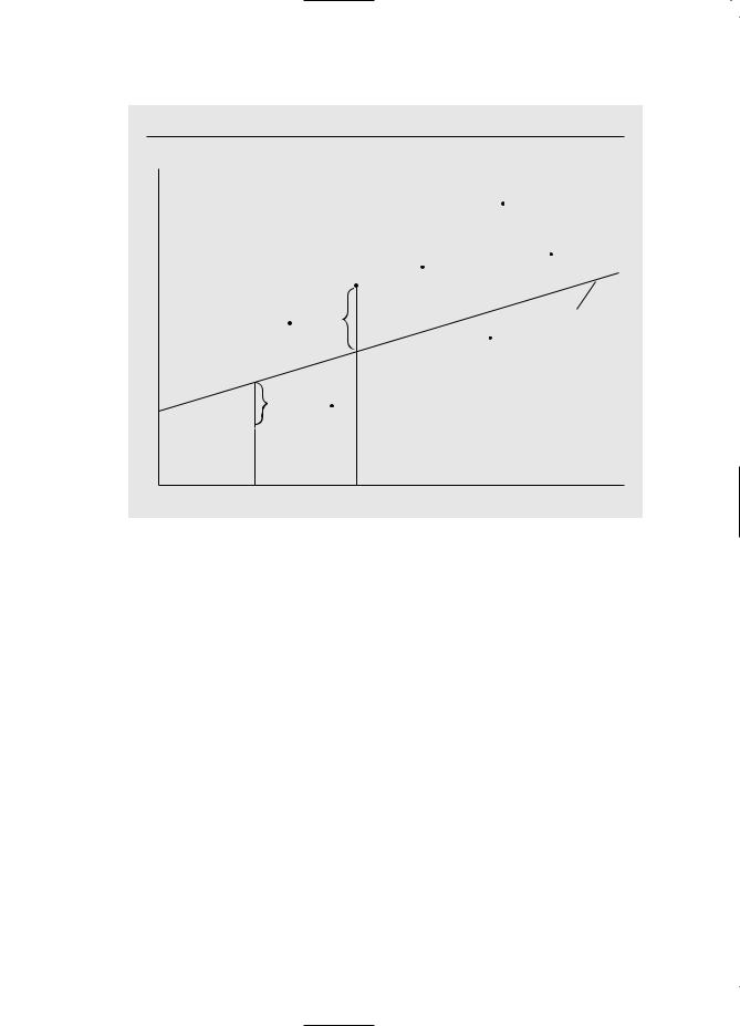
The relationship (2.48) can be plotted for a particular outcome of data as shown in Figure 2.7.

In order to obtain unbiased estimators of 0 and 1, we need to impose the zero conditional mean assumption that we discussed in some detail in Section 2.1. We now explicitly add it to our list of assumptions.

A S S U M P T I O N S L R . 3 ( Z E R O C O N D I T I O N A L M E A N )

E(u x) 0.

47

Part 1 Regression Analysis with Cross-Sectional Data

F i g u r e 2 . 7

Graph of yi 0 1xi ui.

y

u1

y1

For a random sample, this assumption implies that E(ui xi) 0, for all i 1,2,…,n. In addition to restricting the relationship between u and x in the population, the zero

conditional mean assumption—coupled with the random sampling assumption— allows for a convenient technical simplification. In particular, we can derive the statistical properties of the OLS estimators as conditional on the values of the xi in our sample. Technically, in statistical derivations, conditioning on the sample values of the independent variable is the same as treating the xi as fixed in repeated samples. This process involves several steps. We first choose n sample values for x1, x2, …, xn (These can be repeated.). Given these values, we then obtain a sample on y (effectively by obtaining a random sample of the ui). Next another sample of y is obtained, using the same values for x1, …, xn. Then another sample of y is obtained, again using the same xi. And so on.

The fixed in repeated samples scenario is not very realistic in nonexperimental contexts. For instance, in sampling individuals for the wage-education example, it makes little sense to think of choosing the values of educ ahead of time and then sampling individuals with those particular levels of education. Random sampling, where individuals are chosen randomly and their wage and education are both recorded, is representative of how most data sets are obtained for empirical analysis in the social sciences. Once we assume that E(u x) 0, and we have random sampling, nothing is lost in derivations by treating the xi as nonrandom. The danger is that the fixed in repeated samples assumption always implies that ui and xi are independent. In deciding when

48

simple regression analysis is going to produce unbiased estimators, it is critical to think in terms of Assumption SLR.3.

Once we have agreed to condition on the xi, we need one final assumption for unbiasedness.

In the sample, the independent variables xi, i 1,2,…,n, are not all equal to the same constant. This requires some variation in x in the population.

We encountered Assumption SLR.4 when we derived the formulas for the OLS esti-

n

mators; it is equivalent to (xi x¯)2 0. Of the four assumptions made, this is the

i 1

least important because it essentially never fails in interesting applications. If Assumption SLR.4 does fail, we cannot compute the OLS estimators, which means statistical analysis is irrelevant.

Because we are now interested in the behavior of ˆ1 across all possible samples, ˆ1 is properly viewed as a random variable.

We can write ˆ1 in terms of the population coefficients and errors by substituting the right hand side of (2.48) into (2.49). We have

n

where we have defined the total variation in xi as sx2 (xi x¯)2 in order to simplify

i 1

the notation. (This is not quite the sample variance of the xi because we do not divide by n 1.) Using the algebra of the summation operator, write the numerator of ˆ1 as

49

where di xi x¯. We now see that the estimator ˆ1 equals the population slope 1, plus a term that is a linear combination in the errors {u1,u2,…,un}. Conditional on the values of xi, the randomness in ˆ1 is due entirely to the errors in the sample. The fact that these errors are generally different from zero is what causes ˆ1 to differ from 1.

Using the representation in (2.52), we can prove the first important statistical property of OLS.

T H E O R E M 2 . 1 ( U N B I A S E D N E S S O F O L S )

Using Assumptions SLR.1 through SLR.4,

P R O O F : In this proof, the expected values are conditional on the sample values of the independent variable. Since sx2 and di are functions only of the xi, they are nonrandom in the conditioning. Therefore, from (2.53),

where we have used the fact that the expected value of each ui (conditional on {x1,x2,...,xn}) is zero under Assumptions SLR.2 and SLR.3.

The proof for ˆ is now straightforward. Average (2.48) across i to get y¯ x¯

0 0 1

u¯, and plug this into the formula for ˆ :

0

implies that E[( 1 1)] 0. Thus, E( 0) 0. Both of these arguments are valid for any values of 0 and 1, and so we have established unbiasedness.

50