Wooldridge_-_Introductory_Econometrics_2nd_Ed

n 526, R2 .186.

This is only the result from a single sample, so we cannot say that .083 is greater than 1; the true return to education could be lower or higher than 8.3 percent (and we will never know for sure). Nevertheless, we know that the average of the estimates across all random samples would be too large.

As a second example, suppose that, at the elementary school level, the average score for students on a standardized exam is determined by

avgscore 0 1expend 2povrate u,

where expend is expenditure per student and povrate is the poverty rate of the children in the school. Using school district data, we only have observations on the percent of students with a passing grade and per student expenditures; we do not have information on poverty rates. Thus, we estimate 1 from the simple regression of avgscore on expend.

We can again obtain the likely bias in ˜1. First, 2 is probably negative: there is ample evidence that children living in poverty score lower, on average, on standardized tests. Second, the average expenditure per student is probably negatively correlated with the poverty rate: the higher the poverty rate, the lower the average per-student spending, so that Corr(x1,x2) 0. From Table 3.2, ˜1 will have a positive bias. This observation has important implications. It could be that the true effect of spending is zero; that is, 1 0. However, the simple regression estimate of 1 will usually be greater than zero, and this could lead us to conclude that expenditures are important when they are not.

When reading and performing empirical work in economics, it is important to master the terminology associated with biased estimators. In the context of omitting a variable from model (3.40), if E( ˜1) 1, then we say that ˜1 has an upward bias. When E( ˜1) 1, ˜1 has a downward bias. These definitions are the same whether 1 is positive or negative. The phrase biased towards zero refers to cases where E( ˜1) is closer to zero than 1. Therefore, if 1 is positive, then ˜1 is biased towards zero if it has a downward bias. On the other hand, if 1 0, then ˜1 is biased towards zero if it has an upward bias.

Omitted Variable Bias: More General Cases

Deriving the sign of omitted variable bias when there are multiple regressors in the estimated model is more difficult. We must remember that correlation between a single explanatory variable and the error generally results in all OLS estimators being biased. For example, suppose the population model

satisfies Assumptions MLR.1 through MLR.4. But we omit x3 and estimate the model as

91

Part 1 Regression Analysis with Cross-Sectional Data

Now, suppose that x2 and x3 are uncorrelated, but that x1 is correlated with x3. In other words, x1 is correlated with the omitted variable, but x2 is not. It is tempting to think that, while ˜1 is probably biased based on the derivation in the previous subsection, ˜2 is unbiased because x2 is uncorrelated with x3. Unfortunately, this is not generally the case: both ˜1 and ˜2 will normally be biased. The only exception to this is when x1 and x2 are also uncorrelated.

Even in the fairly simple model above, it is difficult to obtain the direction of the bias in ˜1 and ˜2. This is because x1, x2, and x3 can all be pairwise correlated. Nevertheless, an approximation is often practically useful. If we assume that x1 and x2 are uncorrelated, then we can study the bias in ˜1 as if x2 were absent from both the population and the estimated models. In fact, when x1 and x2 are uncorrelated, it can be shown that

i 1

This is just like equation (3.46), but 3 replaces 2 and x3 replaces x2. Therefore, the bias

As an example, suppose we add exper to the wage model:

wage 0 1educ 2exper 3abil u.

If abil is omitted from the model, the estimators of both 1 and 2 are biased, even if we assume exper is uncorrelated with abil. We are mostly interested in the return to education, so it would be nice if we could conclude that ˜1 has an upward or downward bias due to omitted ability. This conclusion is not possible without further assumptions. As an approximation, let us suppose that, in addition to exper and abil being uncorrelated, educ and exper are also uncorrelated. (In reality, they are somewhat negatively correlated.) Since 3 0 and educ and abil are positively correlated, ˜1 would have an upward bias, just as if exper were not in the model.

The reasoning used in the previous example is often followed as a rough guide for obtaining the likely bias in estimators in more complicated models. Usually, the focus is on the relationship between a particular explanatory variable, say x1, and the key omitted factor. Strictly speaking, ignoring all other explanatory variables is a valid practice only when each one is uncorrelated with x1, but it is still a useful guide.

3.4 THE VARIANCE OF THE OLS ESTIMATORS

We now obtain the variance of the OLS estimators so that, in addition to knowing the central tendencies of ˆj, we also have a measure of the spread in its sampling distribution. Before finding the variances, we add a homoskedasticity assumption, as in Chapter 2. We do this for two reasons. First, the formulas are simplified by imposing the con-

92

stant error variance assumption. Second, in Section 3.5, we will see that OLS has an important efficiency property if we add the homoskedasticity assumption.

In the multiple regression framework, homoskedasticity is stated as follows:

A S S U M P T I O N M L R . 5 ( H O M O S K E D A S T I C I T Y )

Var(u x1,…, xk) 2.

Assumption MLR.5 means that the variance in the error term, u, conditional on the explanatory variables, is the same for all combinations of outcomes of the explanatory variables. If this assumption fails, then the model exhibits heteroskedasticity, just as in the two-variable case.

In the equation

wage 0 1educ 2exper 3tenure u,

homoskedasticity requires that the variance of the unobserved error u does not depend on the levels of education, experience, or tenure. That is,

Var(u educ, exper, tenure) 2.

If this variance changes with any of the three explanatory variables, then heteroskedasticity is present.

Assumptions MLR.1 through MLR.5 are collectively known as the Gauss-Markov assumptions (for cross-sectional regression). So far, our statements of the assumptions are suitable only when applied to cross-sectional analysis with random sampling. As we will see, the Gauss-Markov assumptions for time series analysis, and for other situations such as panel data analysis, are more difficult to state, although there are many similarities.

In the discussion that follows, we will use the symbol x to denote the set of all independent variables, (x1, …, xk). Thus, in the wage regression with educ, exper, and tenure as independent variables, x (educ, exper, tenure). Now we can write Assumption MLR.3 as

E(y x) 0 1x1 2x2 … kxk,

and Assumption MLR.5 is the same as Var(y x) 2. Stating the two assumptions in this way clearly illustrates how Assumption MLR.5 differs greatly from Assumption MLR.3. Assumption MLR.3 says that the expected value of y, given x, is linear in the parameters, but it certainly depends on x1, x2, …, xk. Assumption MLR.5 says that the variance of y, given x, does not depend on the values of the independent variables.

We can now obtain the variances of the ˆj, where we again condition on the sample values of the independent variables. The proof is in the appendix to this chapter.

T H E O R E M 3 . 2 ( S A M P L I N G V A R I A N C E S O F T H E O L S S L O P E E S T I M A T O R S )

Under Assumptions MLR.1 through MLR.5, conditional on the sample values of the independent variables,

93

Part 1 Regression Analysis with Cross-Sectional Data

n

for j 1,2,…,k, where SSTj (xij x¯j)2 is the total sample variation in xj, and R2j is

i 1

the R-squared from regressing xj on all other independent variables (and including an intercept).

Before we study equation (3.51) in more detail, it is important to know that all of the Gauss-Markov assumptions are used in obtaining this formula. While we did not need the homoskedasticity assumption to conclude that OLS is unbiased, we do need it to validate equation (3.51).

The size of Var( ˆj) is practically important. A larger variance means a less precise estimator, and this translates into larger confidence intervals and less accurate hypotheses tests (as we will see in Chapter 4). In the next subsection, we discuss the elements comprising (3.51).

The Components of the OLS Variances: Multicollinearity

Equation (3.51) shows that the variance of ˆj depends on three factors: 2, SSTj, and Rj2. Remember that the index j simply denotes any one of the independent variables (such as education or poverty rate). We now consider each of the factors affecting Var( ˆj) in turn.

THE ERROR VARIANCE, 2. From equation (3.51), a larger 2 means larger variances for the OLS estimators. This is not at all surprising: more “noise” in the equation (a larger 2) makes it more difficult to estimate the partial effect of any of the independent variables on y, and this is reflected in higher variances for the OLS slope estimators. Since 2 is a feature of the population, it has nothing to do with the sample size. It is the one component of (3.51) that is unknown. We will see later how to obtain an unbiased estimator of 2.

For a given dependent variable y, there is really only one way to reduce the error variance, and that is to add more explanatory variables to the equation (take some factors out of the error term). This is not always possible, nor is it always desirable for reasons discussed later in the chapter.

THE TOTAL SAMPLE VARIATION IN xj, SSTj. From equation (3.51), the larger the total variation in xj, the smaller is Var( ˆj). Thus, everything else being equal, for estimating j we prefer to have as much sample variation in xj as possible. We already discovered this in the simple regression case in Chapter 2. While it is rarely possible for us to choose the sample values of the independent variables, there is a way to increase the sample variation in each of the independent variables: increase the sample size. In fact, when sampling randomly from a population, SSTj increases without bound as the sample size gets larger and larger. This is the component of the variance that systematically depends on the sample size.

94

When SSTj is small, Var( ˆj) can get very large, but a small SSTj is not a violation of Assumption MLR.4. Technically, as SSTj goes to zero, Var( ˆj) approaches infinity. The extreme case of no sample variation in xj, SSTj 0, is not allowed by Assumption MLR.4.

THE LINEAR RELATIONSHIPS AMONG THE INDEPENDENT VARIABLES, Rj2. The term Rj2 in equation (3.51) is the most difficult of the three components to understand. This term does not appear in simple regression analysis because there is only one independent variable in such cases. It is important to see that this R-squared is distinct from the R-squared in the regression of y on x1, x2, …, xk: Rj2 is obtained from a regression involving only the independent variables in the original model, where xj plays the role of a dependent variable.

Consider first the k 2 case: y 0 1x1 2x2 u. Then Var( ˆ1)2/[SST1(1 R12)], where R12 is the R-squared from the simple regression of x1 on x2

(and an intercept, as always). Since the R-squared measures goodness-of-fit, a value of R12 close to one indicates that x2 explains much of the variation in x1 in the sample. This means that x1 and x2 are highly correlated.

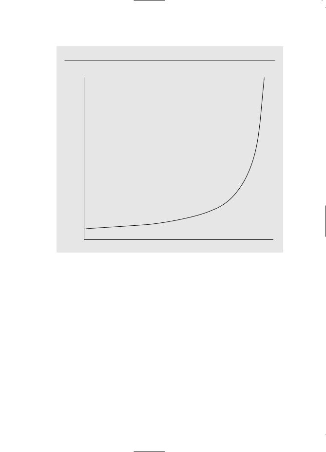
As R12 increases to one, Var( ˆ1) gets larger and larger. Thus, a high degree of linear relationship between x1 and x2 can lead to large variances for the OLS slope estimators. (A similar argument applies to ˆ2.) See Figure 3.1 for the relationship between Var( ˆ1) and the R-squared from the regression of x1 on x2.

In the general case, Rj2 is the proportion of the total variation in xj that can be explained by the other independent variables appearing in the equation. For a given 2 and SSTj, the smallest Var( ˆj) is obtained when Rj2 0, which happens if, and only if, xj has zero sample correlation with every other independent variable. This is the best case for estimating j, but it is rarely encountered.

The other extreme case, Rj2 1, is ruled out by Assumption MLR.4, because Rj2 1 means that, in the sample, xj is a perfect linear combination of some of the other independent variables in the regression. A more relevant case is when Rj2 is “close” to one. From equation (3.51) and Figure 3.1, we see that this can cause Var( ˆj) to be large: Var( ˆj) * as Rj2 * 1. High (but not perfect) correlation between two or more of the independent variables is called multicollinearity.

Before we discuss the multicollinearity issue further, it is important to be very clear on one thing: a case where Rj2 is close to one is not a violation of Assumption MLR.4.

Since multicollinearity violates none of our assumptions, the “problem” of multicollinearity is not really well-defined. When we say that multicollinearity arises for estimating j when Rj2 is “close” to one, we put “close” in quotation marks because there is no absolute number that we can cite to conclude that multicollinearity is a problem. For example, Rj2 .9 means that 90 percent of the sample variation in xj can be explained by the other independent variables in the regression model. Unquestionably, this means that xj has a strong linear relationship to the other independent variables. But whether this translates into a Var( ˆj) that is too large to be useful depends on the sizes of 2 and SSTj. As we will see in Chapter 4, for statistical inference, what ultimately matters is how big ˆj is in relation to its standard deviation.

Just as a large value of Rj2 can cause large Var( ˆj), so can a small value of SSTj. Therefore, a small sample size can lead to large sampling variances, too. Worrying

95

Part 1 Regression Analysis with Cross-Sectional Data

F i g u r e 3 . 1

Var ( ˆ1) as a function of R12.

Var ( ˆ 1)

about high degrees of correlation among the independent variables in the sample is really no different from worrying about a small sample size: both work to increase Var( ˆj). The famous University of Wisconsin econometrician Arthur Goldberger, reacting to econometricians’ obsession with multicollinearity, has [tongue-in-cheek] coined the term micronumerosity, which he defines as the “problem of small sample size.” [For an engaging discussion of multicollinearity and micronumerosity, see Goldberger (1991).]

Although the problem of multicollinearity cannot be clearly defined, one thing is clear: everything else being equal, for estimating j it is better to have less correlation between xj and the other independent variables. This observation often leads to a discussion of how to “solve” the multicollinearity problem. In the social sciences, where we are usually passive collectors of data, there is no good way to reduce variances of unbiased estimators other than to collect more data. For a given data set, we can try dropping other independent variables from the model in an effort to reduce multicollinearity. Unfortunately, dropping a variable that belongs in the population model can lead to bias, as we saw in Section 3.3.

Perhaps an example at this point will help clarify some of the issues raised concerning multicollinearity. Suppose we are interested in estimating the effect of various

96

school expenditure categories on student performance. It is likely that expenditures on teacher salaries, instructional materials, athletics, and so on, are highly correlated: wealthier schools tend to spend more on everything, and poorer schools spend less on everything. Not surprisingly, it can be difficult to estimate the effect of any particular expenditure category on student performance when there is little variation in one category that cannot largely be explained by variations in the other expenditure categories (this leads to high Rj2 for each of the expenditure variables). Such multicollinearity problems can be mitigated by collecting more data, but in a sense we have imposed the problem on ourselves: we are asking questions that may be too subtle for the available data to answer with any precision. We can probably do much better by changing the scope of the analysis and lumping all expenditure categories together, since we would no longer be trying to estimate the partial effect of each separate category.

Another important point is that a high degree of correlation between certain independent variables can be irrelevant as to how well we can estimate other parameters in the model. For example, consider a model with three independent variables:

y 0 1x1 2x2 3x3 u,

where x2 and x3 are highly correlated. Then Var( ˆ2) and Var( ˆ3) may be large. But the amount of correlation between x2 and x3 has no direct effect on Var( ˆ1). In fact, if x1 is uncorrelated with x2 and x3, then R12 0 and Var( ˆ1) 2/SST1, regardless of how much correlation there is between x2 and x3. If 1 is the parameter of interest, we do not really care about the amount of correlation

between x2 and x3.

The previous observation is important because economists often include many controls in order to isolate the causal effect of a particular variable. For example, in looking at the relationship between loan approval rates and percent of minorities in a neighborhood, we might include variables like average income, average housing value, measures of creditworthiness,

and so on, because these factors need to be accounted for in order to draw causal conclusions about discrimination. Income, housing prices, and creditworthiness are generally highly correlated with each other. But high correlations among these variables do not make it more difficult to determine the effects of discrimination.

Variances in Misspecified Models

The choice of whether or not to include a particular variable in a regression model can be made by analyzing the tradeoff between bias and variance. In Section 3.3, we derived the bias induced by leaving out a relevant variable when the true model contains two explanatory variables. We continue the analysis of this model by comparing the variances of the OLS estimators.

Write the true population model, which satisfies the Gauss-Markov assumptions, as

y 0 1x1 2x2 u.

97

We consider two estimators of 1. The estimator ˆ1 comes from the multiple regression

In other words, we include x2, along with x1, in the regression model. The estimator ˜1 is obtained by omitting x2 from the model and running a simple regression of y on x1:

When 2 0, equation (3.53) excludes a relevant variable from the model and, as we saw in Section 3.3, this induces a bias in ˜1 unless x1 and x2 are uncorrelated. On the other hand, ˆ1 is unbiased for 1 for any value of 2, including 2 0. It follows that, if bias is used as the only criterion, ˆ1 is preferred to ˜1.

The conclusion that ˆ1 is always preferred to ˜1 does not carry over when we bring variance into the picture. Conditioning on the values of x1 and x2 in the sample, we have, from (3.51),

where SST1 is the total variation in x1, and R12 is the R-squared from the regression of x1 on x2. Further, a simple modification of the proof in Chapter 2 for two-variable regression shows that

Comparing (3.55) to (3.54) shows that Var( ˜1) is always smaller than Var( ˆ1), unless x1 and x2 are uncorrelated in the sample, in which case the two estimators ˜1 and ˆ1 are the same. Assuming that x1 and x2 are not uncorrelated, we can draw the following conclusions:

1.When 2 0, ˜1 is biased, ˆ1 is unbiased, and Var( ˜1) Var( ˆ1).

2.When 2 0, ˜1 and ˆ1 are both unbiased, and Var( ˜1) Var( ˆ1).

From the second conclusion, it is clear that ˜1 is preferred if 2 0. Intuitively, if x2 does not have a partial effect on y, then including it in the model can only exacerbate the multicollinearity problem, which leads to a less efficient estimator of 1. A higher variance for the estimator of 1 is the cost of including an irrelevant variable in a model.

The case where 2 0 is more difficult. Leaving x2 out of the model results in a biased estimator of 1. Traditionally, econometricians have suggested comparing the likely size of the bias due to omitting x2 with the reduction in the variance—summa- rized in the size of R12—to decide whether x2 should be included. However, when2 0, there are two favorable reasons for including x2 in the model. The most important of these is that any bias in ˜1 does not shrink as the sample size grows; in fact, the bias does not necessarily follow any pattern. Therefore, we can usefully think of the bias as being roughly the same for any sample size. On the other hand, Var( ˜1) and Var( ˆ1) both shrink to zero as n gets large, which means that the multicollinearity induced by adding x2 becomes less important as the sample size grows. In large samples, we would prefer ˆ1.

98

The other reason for favoring ˆ1 is more subtle. The variance formula in (3.55) is conditional on the values of xi1 and xi2 in the sample, which provides the best scenario for ˜1. When 2 0, the variance of ˜1 conditional only on x1 is larger than that presented in (3.55). Intuitively, when 2 0 and x2 is excluded from the model, the error variance increases because the error effectively contains part of x2. But formula (3.55) ignores the error variance increase because it treats both regressors as nonrandom. A full discussion of which independent variables to condition on would lead us too far astray. It is sufficient to say that (3.55) is too generous when it comes to measuring the precision in ˜1.

Estimating 2: Standard Errors of the OLS Estimators

We now show how to choose an unbiased estimator of 2, which then allows us to obtain unbiased estimators of Var( ˆj).

Since 2 E(u2), an unbiased “estimator” of 2 is the sample average of the

n

squared errors: n-1 u2i . Unfortunately, this is not a true estimator because we do not

i 1

observe the ui. Nevertheless, recall that the errors can be written as ui yi 0 1xi1

2xi2 … kxik, and so the reason we do not observe the ui is that we do not know the j. When we replace each j with its OLS estimator, we get the OLS residuals:

uˆi yi ˆ0 ˆ1xi1 ˆ2xi2 … ˆkxik.

It seems natural to estimate 2 by replacing ui with the uˆi. In the simple regression case, we saw that this leads to a biased estimator. The unbiased estimator of 2 in the general multiple regression case is

We already encountered this estimator in the k 1 case in simple regression.

The term n k 1 in (3.56) is the degrees of freedom (df ) for the general OLS problem with n observations and k independent variables. Since there are k 1 parameters in a regression model with k independent variables and an intercept, we can write

df n (k 1)

This is the easiest way to compute the degrees of freedom in a particular application: count the number of parameters, including the intercept, and subtract this amount from the number of observations. (In the rare case that an intercept is not estimated, the number of parameters decreases by one.)

Technically, the division by n k 1 in (3.56) comes from the fact that the expected value of the sum of squared residuals is E(SSR) (n k 1) 2. Intuitively,

we can figure out why the degrees of freedom adjustment is necessary by returning to

n

the first order conditions for the OLS estimators. These can be written as uˆi 0 and

i 1

99

n

xijuˆi 0, where j 1,2, …, k. Thus, in obtaining the OLS estimates, k 1 restric-

i 1

tions are imposed on the OLS residuals. This means that, given n (k 1) of the residuals, the remaining k 1 residuals are known: there are only n (k 1) degrees of freedom in the residuals. (This can be contrasted with the errors ui, which have n degrees of freedom in the sample.)

For reference, we summarize this discussion with Theorem 3.3. We proved this theorem for the case of simple regression analysis in Chapter 2 (see Theorem 2.3). (A general proof that requires matrix algebra is provided in Appendix E.)

T H E O R E M 3 . 3 ( U N B I A S E D E S T I M A T I O N O F 2 )

Under the Gauss-Markov Assumptions MLR.1 through MLR.5, E( ˆ 2) 2.

The positive square root of ˆ 2, denoted ˆ, is called the standard error of the regression or SER. The SER is an estimator of the standard deviation of the error term. This estimate is usually reported by regression packages, although it is called different things by different packages. (In addition to ser, ˆ is also called the standard error of the estimate and the root mean squared error.)

Note that ˆ can either decrease or increase when another independent variable is added to a regression (for a given sample). This is because, while SSR must fall when another explanatory variable is added, the degrees of freedom also falls by one. Because SSR is in the numerator and df is in the denominator, we cannot tell beforehand which effect will dominate.

For constructing confidence intervals and conducting tests in Chapter 4, we need to estimate the standard deviation of ˆj, which is just the square root of the variance:

sd( ˆj) /[SSTj(1 Rj2)]1/2.

Since is unknown, we replace it with its estimator, ˆ . This gives us the standard error of ˆj:

Just as the OLS estimates can be obtained for any given sample, so can the standard errors. Since se( ˆj) depends on ˆ , the standard error has a sampling distribution, which will play a role in Chapter 4.

We should emphasize one thing about standard errors. Because (3.58) is obtained directly from the variance formula in (3.51), and because (3.51) relies on the homoskedasticity Assumption MLR.5, it follows that the standard error formula in (3.58) is not a valid estimator of sd( ˆj) if the errors exhibit heteroskedasticity. Thus, while the presence of heteroskedasticity does not cause bias in the ˆj, it does lead to bias in the usual formula for Var( ˆj), which then invalidates the standard errors. This is important because any regression package computes (3.58) as the default standard error for each coefficient (with a somewhat different representation for the intercept). If we suspect heteroskedasticity, then the “usual” OLS standard errors are invalid and some corrective action should be taken. We will see in Chapter 8 what methods are available for dealing with heteroskedasticity.

100