Wooldridge_-_Introductory_Econometrics_2nd_Ed

strength for Candidate A (the percent of the most recent presidential vote that went to A’s party).

(i)What is the interpretation of 1?

(ii)In terms of the parameters, state the null hypothesis that a 1% increase in A’s expenditures is offset by a 1% increase in B’s expenditures.

(iii)Estimate the model above using the data in VOTE1.RAW and report the results in usual form. Do A’s expenditures affect the outcome? What about B’s expenditures? Can you use these results to test the hypothesis in part (ii)?

(iv)Estimate a model that directly gives the t statistic for testing the hypothesis in part (ii). What do you conclude? (Use a two-sided alternative.)

4.13Use the data in LAWSCH85.RAW for this exercise.

(i)Using the same model as Problem 3.4, state and test the null hypothesis that the rank of law schools has no ceteris paribus effect on median starting salary.

(ii)Are features of the incoming class of students—namely, LSAT and GPA—individually or jointly significant for explaining salary?

(iii)Test whether the size of the entering class (clsize) or the size of the faculty ( faculty) need to be added to this equation; carry out a single test. (Be careful to account for missing data on clsize and faculty.)

(iv)What factors might influence the rank of the law school that are not included in the salary regression?

4.14Refer to Problem 3.14. Now, use the log of the housing price as the dependent variable:

log(price) 0 1sqrft 2bdrms u.

(i)You are interested in estimating and obtaining a confidence interval for the percentage change in price when a 150-square-foot bedroom is

added to a house. In decimal form, this is 1 150 1 2. Use the data in HPRICE1.RAW to estimate 1.

(ii)Write 2 in terms of 1 and 1 and plug this into the log(price) equation.

(iii)Use part (ii) to obtain a standard error for ˆ1 and use this standard error to construct a 95% confidence interval.

4.15In Example 4.9, the restricted version of the model can be estimated using all 1,388 observations in the sample. Compute the R-squared from the regression of bwght on cigs, parity, and faminc using all observations. Compare this to the R-squared reported for the restricted model in Example 4.9.

4.16Use the data in MLB1.RAW for this exercise.

(i)Use the model estimated in equation (4.31) and drop the variable rbisyr. What happens to the statistical significance of hrunsyr? What about the size of the coefficient on hrunsyr?

(ii)Add the variables runsyr, fldperc, and sbasesyr to the model from part

(i). Which of these factors are individually significant?

(iii)In the model from part (ii), test the joint significance of bavg, fldperc, and sbasesyr.

160

4.17Use the data in WAGE2.RAW for this exercise.

(i)Consider the standard wage equation

log(wage) 0 1educ 2exper 3tenure u.

State the null hypothesis that another year of general workforce experience has the same effect on log(wage) as another year of tenure with the current employer.

(ii)Test the null hypothesis in part (i) against a two-sided alternative, at the 5% significance level, by constructing a 95% confidence interval. What do you conclude?

161

C h a p t e r Five

Multiple Regression Analysis:

OLS Asymptotics

In Chapters 3 and 4, we covered what are called finite sample, small sample, or exact properties of the OLS estimators in the population model

For example, the unbiasedness of OLS (derived in Chapter 3) under the first four GaussMarkov assumptions is a finite sample property because it holds for any sample size n (subject to the mild restriction that n must be at least as large as the total number of parameters in the regression model, k 1). Similarly, the fact that OLS is the best linear unbiased estimator under the full set of Gauss-Markov assumptions (MLR.1 through MLR.5) is a finite sample property.

In Chapter 4, we added the classical linear model Assumption MLR.6, which states that the error term u is normally distributed and independent of the explanatory variables. This allowed us to derive the exact sampling distributions of the OLS estimators (conditional on the explanatory variables in the sample). In particular, Theorem 4.1 showed that the OLS estimators have normal sampling distributions, which led directly to the t and F distributions for t and F statistics. If the error is not normally distributed, the distribution of a t statistic is not exactly t, and an F statistic does not have an exact F distribution for any sample size.

In addition to finite sample properties, it is important to know the asymptotic properties or large sample properties of estimators and test statistics. These properties are not defined for a particular sample size; rather, they are defined as the sample size grows without bound. Fortunately, under the assumptions we have made, OLS has satisfactory large sample properties. One practically important finding is that even without the normality assumption (Assumption MLR.6), t and F statistics have approximately t and F distributions, at least in large sample sizes. We discuss this in more detail in Section 5.2, after we cover consistency of OLS in Section 5.1.

5.1 CONSISTENCY

Unbiasedness of estimators, while important, cannot always be achieved. For example, as we discussed in Chapter 3, the standard error of the regression, ˆ, is not an unbiased

162

estimator for , the standard deviation of the error u in a multiple regression model. While the OLS estimators are unbiased under MLR.1 through MLR.4, in Chapter 11 we will find that there are time series regressions where the OLS estimators are not unbiased. Further, in Part 3 of the text, we encounter several other estimators that are biased.

While not all useful estimators are unbiased, virtually all economists agree that consistency is a minimal requirement for an estimator. The famous econometrician Clive W.J. Granger once remarked: “If you can’t get it right as n goes to infinity, you shouldn’t be in this business.” The implication is that, if your estimator of a particular population parameter is not consistent, then you are wasting your time.

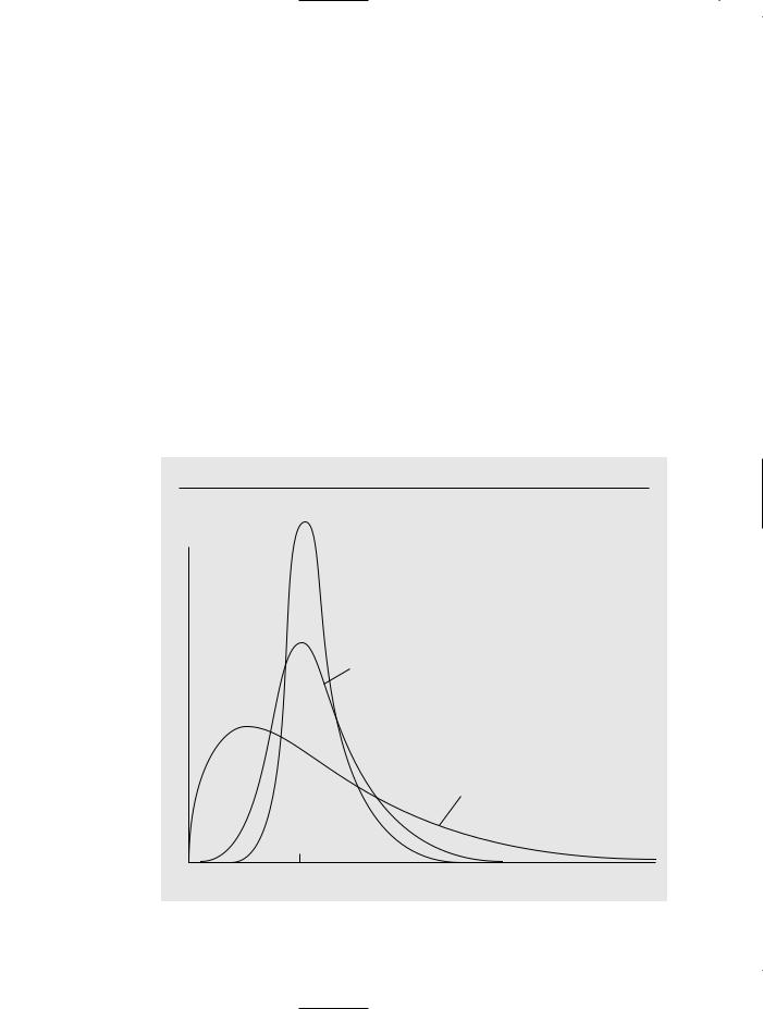
There are a few different ways to describe consistency. Formal definitions and results are given in Appendix C; here we focus on an intuitive understanding. For concreteness, let ˆj be the OLS estimator of j for some j. For each n, ˆj has a probability distribution (representing its possible values in different random samples of size n). Because ˆj is unbiased under assumptions MLR.1 through MLR.4, this distribution has mean value j. If this estimator is consistent, then the distribution of ˆj becomes more and more tightly distributed around j as the sample size grows. As n tends to infinity, the distribution of ˆj collapses to the single point j. In effect, this means that we can make our estimator arbitrarily close to j if we can collect as much data as we want. This convergence is illustrated in Figure 5.1.

F i g u r e 5 . 1

Sampling distributions of ˆ1 for sample sizes n1 n2 n3.

n3 fˆ 1

n2

n1

163

Naturally, for any application we have a fixed sample size, which is the reason an asymptotic property such as consistency can be difficult to grasp. Consistency involves a thought experiment about what would happen as the sample size gets large (while at the same time we obtain numerous random samples for each sample size). If obtaining more and more data does not generally get us closer to the parameter value of interest, then we are using a poor estimation procedure.

Conveniently, the same set of assumptions imply both unbiasedness and consistency of OLS. We summarize with a theorem.

T H E O R E M 5 . 1 ( C O N S I S T E N C Y O F O L S )

Under assumptions MLR.1 through MLR.4, the OLS estimator ˆj is consistent for j, for all j 0,1, …, k.

A general proof of this result is most easily developed using the matrix algebra methods described in Appendices D and E. But we can prove Theorem 5.1 without difficulty in the case of the simple regression model. We focus on the slope estimator, ˆ1.

The proof starts out the same as the proof of unbiasedness: we write down the formula for ˆ1, and then plug in yi 0 1xi1 ui:

We can apply the law of large numbers to the numerator and denominator, which converge in probability to the population quantities, Cov(x1,u) and Var(x1), respectively. Provided that Var(x1) 0—which is assumed in MLR.4—we can use the properties of probability limits (see Appendix C) to get

plim ˆ1 1 Cov(x1,u)/Var(x1)

1, because Cov(x1,u) 0.

(5.3)

We have used the fact, discussed in Chapters 2 and 3, that E(u x1) 0 implies that x1 and u are uncorrelated (have zero covariance).

As a technical matter, to ensure that the probability limits exist, we should assume that Var(x1) and Var(u) (which means that their probability distributions are not too spread out), but we will not worry about cases where these assumptions might fail.

The previous arguments, and equation (5.3) in particular, show that OLS is consistent in the simple regression case if we assume only zero correlation. This is also true in the general case. We now state this as an assumption.

A S S U M P T I O N M L R . 3 ( Z E R O M E A N A N D Z E R O

C O R R E L A T I O N )

E(u) 0 and Cov(xj,u) 0, for j 1,2, …, k.

164

In Chapter 3, we discussed why assumption MLR.3 implies MLR.3 , but not vice versa. The fact that OLS is consistent under the weaker assumption MLR.3 turns out to be useful in Chapter 15 and in other situations. Interestingly, while OLS is unbiased under MLR.3, this is not the case under Assumption MLR.3 . (This was the leading reason we have assumed MLR.3.)

Deriving the Inconsistency in OLS

Just as failure of E(u x1, …, xk) 0 causes bias in the OLS estimators, correlation between u and any of x1, x2, …, xk generally causes all of the OLS estimators to be inconsistent. This simple but important observation is often summarized as: if the error is correlated with any of the independent variables, then OLS is biased and inconsistent. This is very unfortunate because it means that any bias persists as the sample size grows.

In the simple regression case, we can obtain the inconsistency from equation (5.3), which holds whether or not u and x1 are uncorrelated. The inconsistency in ˆ1 (sometimes loosely called the asymptotic bias) is

Because Var(x1) 0, the inconsistency in ˆ1 is positive if x1 and u are positively correlated, and the inconsistency is negative if x1 and u are negatively correlated. If the covariance between x1 and u is small relative to the variance in x1, the inconsistency can be negligible; unfortunately, we cannot even estimate how big the covariance is because u is unobserved.

We can use (5.4) to derive the asymptotic analog of the omitted variable bias (see Table 3.2 in Chapter 3). Suppose the true model,

y 0 1x1 2x2 v,

satisfies the first four Gauss-Markov assumptions. Then v has a zero mean and is uncorrelated with x1 and x2. If ˆ0, ˆ1, and ˆ2 denote the OLS estimators from the regression of y on x1 and x2, then Theorem 5.1 implies that these estimators are consistent. If we omit x2 from the regression and do the simple regression of y on x1, then u 2x2 v. Let ˜1 denote the simple regression slope estimator. Then

Thus, for practical purposes, we can view the inconsistency as being the same as the bias. The difference is that the inconsistency is expressed in terms of the population variance of x1 and the population covariance between x1 and x2, while the bias is based on their sample counterparts (because we condition on the values of x1 and x2 in the sample).

165

If x1 and x2 are uncorrelated (in the population), then 1 0, and ˜1 is a consistent estimator of 1 (although not necessarily unbiased). If x2 has a positive partial effect on y, so that 2 0, and x1 and x2 are positively correlated, so that 1 0, then the inconsistency in ˜1 is positive. And so on. We can obtain the direction of the inconsistency or asymptotic bias from Table 3.2. If the covariance between x1 and x2 is small relative to the variance of x1, the inconsistency can be small.

Let y denote the price of a house (price), let x1 denote the distance from the house to a new trash incinerator (distance), and let x2 denote the “quality” of the house (quality). The variable quality is left vague so that it can include things like size of the house and lot, number of bedrooms and bathrooms, and intangibles such as attractiveness of the neighborhood. If the incinerator depresses house prices, then 1 should be positive: everything else being equal, a house that is farther away from the incinerator is worth more. By definition,2 is positive since higher quality houses sell for more, other factors being equal. If the incinerator was built farther away, on average, from better homes, then distance and quality are positively correlated, and so 1 0. A simple regression of price on distance [or log(price) on log(distance)] will tend to overestimate the effect of the incinerator: 1 2 1 1.

An important point about inconsistency in OLS estimators is that, by definition, the problem does not go away by adding more observations to the sample. If anything, the problem gets worse with more data: the OLS estimator gets closer and closer to

Q U E S T I O N 5 . 1 1 2 1 as the sample size grows. Deriving the sign and magnitude of the

inconsistency in the general k regressor case is much harder, just as deriving the bias is very difficult. We need to remember that if we have the model in equation (5.1) where, say, x1 is correlated with u but the other independent variables are uncorrelated with u, all of the OLS estimators are

generally inconsistent. For example, in the k 2 case,

y 0 1x1 2x2 u,

suppose that x2 and u are uncorrelated but x1 and u are correlated. Then the OLS estimators ˆ1 and ˆ2 will generally both be inconsistent. (The intercept will also be inconsistent.) The inconsistency in ˆ2 arises when x1 and x2 are correlated, as is usually the case. If x1 and x2 are uncorrelated, then any correlation between x1 and u does not result in the inconsistency of ˆ2: plim ˆ2 2. Further, the inconsistency in ˆ1 is the same as in (5.4). The same statement holds in the general case: if x1 is correlated with u, but x1 and u are uncorrelated with the other independent variables, then only ˆ1 is inconsistent, and the inconsistency is given by (5.4).

166

5.2 ASYMPTOTIC NORMALITY AND LARGE SAMPLE INFERENCE

Consistency of an estimator is an important property, but it alone does not allow us to perform statistical inference. Simply knowing that the estimator is getting closer to the population value as the sample size grows does not allow us to test hypotheses about the parameters. For testing, we need the sampling distribution of the OLS estimators. Under the classical linear model assumptions MLR.1 through MLR.6, Theorem 4.1 shows that the sampling distributions are normal. This result is the basis for deriving the t and F distributions that we use so often in applied econometrics.

The exact normality of the OLS estimators hinges crucially on the normality of the distribution of the error, u, in the population. If the errors u1, u2, …, un are random draws from some distribution other than the normal, the ˆj will not be normally distributed, which means that the t statistics will not have t distributions and the F statistics will not have F distributions. This is a potentially serious problem because our inference hinges on being able to obtain critical values or p-values from the t or F distributions.

Recall that Assumption MLR.6 is equivalent to saying that the distribution of y given x1, x2, …, xk is normal. Since y is observed and u is not, in a particular application, it is much easier to think about whether the distribution of y is likely to be normal. In fact, we have already seen a few examples where y definitely cannot have a normal distribution. A normally distributed random variable is symmetrically distributed about its mean, it can take on any positive or negative value (but with zero probability), and more than 95% of the area under the distribution is within two standard deviations.

In Example 3.4, we estimated a model explaining the number of arrests of young men during a particular year (narr86). In the population, most men are not arrested during the year, and the vast majority are arrested one time at the most. (In the sample of 2,725 men in the data set CRIME1.RAW, fewer than 8% were arrested more than once during 1986.) Because narr86 takes on only two values for 92% of the sample, it cannot be close to being normally distributed in the population.

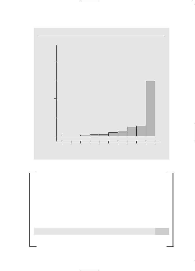
In Example 4.6, we estimated a model explaining participation percentages (prate) in 401(k) pension plans. The frequency distribution (also called a histogram) in Figure 5.2 shows that the distribution of prate is heavily skewed to the right, rather than being normally distributed. In fact, over 40% of the observations on prate are at the value 100, indicating 100% participation. This violates the normality assumption even conditional on the explanatory variables.

We know that normality plays no role in the unbiasedness of OLS, nor does it affect the conclusion that OLS is the best linear unbiased estimator under the GaussMarkov assumptions. But exact inference based on t and F statistics requires MLR.6. Does this mean that, in our analysis of prate in Example 4.6, we must abandon the t statistics for determining which variables are statistically significant? Fortunately, the answer to this question is no. Even though the yi are not from a normal distribution, we can use the central limit theorem from Appendix C to conclude that the OLS estimators are approximately normally distributed, at least in large sample sizes.

167

Part 1 Regression Analysis with Cross-Sectional Data

F i g u r e 5 . 2

Histogram of prate using the data in 401K.RAW.

.8

T H E O R E M 5 . 2 ( A S Y M P T O T I C N O R M A L I T Y

O F O L S )

Under the Gauss-Markov assumptions MLR.1 through MLR.5,

(i) n ( ˆj j) ~ª Normal(0, 2/a2j ), where 2/a2j 0 is the asymptotic variance of

n ( ˆj j); for the slope coefficients, a2j plim n 1 n rˆij2 , where the rˆij are the resid-

i 1

uals from regressing xj on the other independent variables. We say that ˆj is asymptotically normally distributed (see Appendix C);

(ii)ˆ 2 is a consistent estimator of 2 Var(u);

(iii)For each j,

where se( ˆj) is the usual OLS standard error.

168