Добавил:
Upload Опубликованный материал нарушает ваши авторские права? Сообщите нам.
Вуз: Предмет: Файл:
DeBerg_-_Computational_Geometry_-_Algorithms_and_Applications_2e.pdf
Скачиваний:
50
Добавлен:
11.03.2016
Размер:
3 Mб
Скачать

15 Visibility Graphs

Finding the Shortest Route

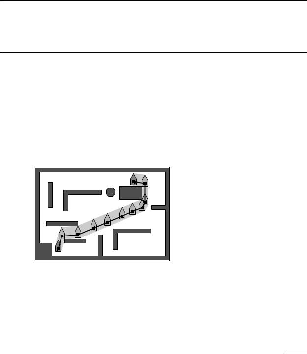
In Chapter 13 we saw how to plan a path for a robot from a given start position to a given goal position. The algorithm we gave always finds a path if it exists, but we made no claims about the quality of the path: it could make a large detour, or make lots of unnecessary turns. In practical situations we would prefer to find not just any path, but a good path.

Figure 15.1

A shortest path

What constitutes a good path depends on the robot. In general, the longer a


path, the more time it will take the robot to reach its goal position. For a mobile


robot on a factory floor this means it can transport less goods per time unit,


resulting in a loss of productivity. Therefore we would prefer a short path. Often


there are other issues that play a role as well. For example, some robots can only


move in a straight line; they have to slow down, stop, and rotate, before they


can start moving into a different direction, so any turn along the path causes


some delay. For this type of robot not only the path length but also the number


of turns on the path has to be taken into account. In this chapter we ignore


this aspect; we only show how to compute the Euclidean shortest path for a


translating planar robot.

323

Chapter 15

VISIBILITY GRAPHS

Figure 15.2

The shortest path does not follow the road map

324

15.1Shortest Paths for a Point Robot

As in Chapter 13 we first consider the case of a point robot moving among a set S of disjoint simple polygons in the plane. The polygons in S are called obstacles, and their total number of edges is denoted by n. Obstacles are open sets, so the robot is allowed to touch them. We are given a start position pstart and a goal position pgoal, which we assume are in the free space. Our goal is to compute a shortest collision-free path from pstart to pgoal, that is, a shortest path that does not intersect the interior of any of the obstacles. Notice that we cannot say the shortest path, because it need not be unique. For a shortest path to exist, it is important that obstacles are open sets; if they were closed, then (unless the robot can move to its goal in a straight line) a shortest path would not exist, as it would always be possible to shorten a path by moving closer to an obstacle.

Let’s quickly review the method from Chapter 13. We computed a trapezoidal map T(Cfree) of the free configuration space Cfree. For a point robot, Cfree was simply the empty space between the obstacles, so this was rather easy. The key idea was then to replace the continuous work space, where there are infinitely many paths, by a discrete road map Groad, where there are only finitely many paths. The road map we used was a plane graph with nodes in the centers of the trapezoids of T(Cfree) and in the middle of the vertical extensions that separate adjacent trapezoids. The nodes in the center of each trapezoid were connected to the nodes on its boundary. After finding the trapezoids containing the start and goal position of the robot, we found a path in the road map between the nodes in the centers of these trapezoids by breadth-first search.

real shortest path

pstart

pgoal

shortest path in road map

Because we used breadth-first search, the path that is found uses a minimum number of arcs in Groad. This is not necessarily a short path, because some arcs are between nodes that are far apart, whereas others are between nodes that are close to each other. An obvious improvement would be to give each arc a weight corresponding to the Euclidean length of the segment connecting its incident nodes, and to use a graph search algorithm that finds a shortest path in a weighted graph, such as Dijkstra’s algorithm. Although this may improve the path length, we still do not get the shortest path. This is illustrated in Figure 15.2:

the shortest path from pstart to pgoal following the road map passes below the triangle, but the real shortest path passes above it. What we need is a different road map, one which guarantees that the shortest path following the road map is the real shortest path.

Let’s see what we can say about the shape of a shortest path. Consider some path from pstart to pgoal. Think of this path as an elastic rubber band, whose endpoints we fix at the start and goal position and which we force to take the shape of the path. At the moment we release the rubber band, it will try to contract and become as short as possible, but it will be stopped by the obstacles. The new path will follow parts of the obstacle boundaries and straight line segments through open space. The next lemma formulates this observation more precisely. It uses the notion of an inner vertex of a polygonal path, which is a vertex that is not the beginor endpoint of the path.

Lemma 15.1 Any shortest path between pstart and pgoal among a set S of disjoint polygonal obstacles is a polygonal path whose inner vertices are vertices of S.

Proof. Suppose for a contradiction that a shortest path τ is not polygonal. Since the obstacles are polygonal, this means there is a point p on τ that lies in the interior of the free space with the property that no line segment containing p is contained in τ . Since p is in the interior of the free space, there is a disc of positive radius centered at p that is completely contained in the free space. But then the part of τ inside the disc, which is not a straight line segment, can be shortened by replacing it with the segment connecting the point where it enters the disc to the point where it leaves the disc. This contradicts the optimality of τ , since any shortest path must be locally shortest, that is, any subpath connecting points q and r on the path must be the shortest path from q to r.

Now consider a vertex v of τ . It cannot lie in the interior of the free space: then there would be a disc centered at p that is completely in the free space, and we could replace the subpath of τ inside the disc— which turns at v—by a straight line segment which is shorter. Similarly, v cannot lie in the relative interior of an obstacle edge: then there would be a disc centered at v such that half of the disc is contained in the free space, which again implies that we can replace the subpath inside the disc with a straight line segment. The only possibility left is that v is an obstacle vertex.

With this characterization of the shortest path, we can construct a road map that allows us to find the shortest path. This road map is the visibility graph of S, which we denote by Gvis(S). Its nodes are the vertices of S, and there is an arc between vertices v and w if they can see each other, that is, if the segment vw does not intersect the interior of any obstacle in S. Two vertices that can see each other are called (mutually) visible, and the segment connecting them is called a visibility edge. Note that endpoints of the same obstacle edge always see each other. Hence, the obstacle edges form a subset of the arcs of Gvis(S).

By Lemma 15.1 the segments on a shortest path are visibility edges, except for the first and last segment. To make them visibility edges as well, we add the start and goal position as vertices to S, that is, we consider the visibility

Section 15.1

SHORTEST PATHS FOR A POINT ROBOT

pgoal

pstart

short cut

p

325

Chapter 15

VISIBILITY GRAPHS

shortest path

pgoal

pstart

graph of the set S := S {pstart, pgoal}. By definition, the arcs of Gvis(S ) are between vertices—which now include pstart and pgoal—that can see each other. We get the following corollary.

Corollary 15.2 The shortest path between pstart and pgoal among a set S of disjoint polygonal obstacles consists of arcs of the visibility graph Gvis(S ),

where S := S {pstart, pgoal}.

We get the following algorithm to compute a shortest path from pstart to pgoal.

Algorithm SHORTESTPATH(S, pstart, pgoal)

Input. A set S of disjoint polygonal obstacles, and two points pstart and pgoal in the free space.

Output. The shortest collision-free path connecting pstart and pgoal.

1.Gvis VISIBILITYGRAPH(S {pstart, pgoal})

2.Assign each arc (v, w) in Gvis a weight, which is the Euclidean length of the segment vw.

3.Use Dijkstra’s algorithm to compute a shortest path between pstart and

pgoal in Gvis.

In the next section we show how to compute the visibility graph in O(n2 log n) time, where n is the total number of obstacle edges. The number of arcs of

Gvis is of course bounded by n+2 . Hence, line 2 of the algorithm takes O(n2)

2

time. Dijkstra’s algorithm computes the shortest path between two nodes in graph with k arcs, each having a non-negative weight, in O(n log n + k) time. Since k = O(n2), we conclude that the total running time of SHORTESTPATH is O(n2 log n), leading to the following theorem.

Theorem 15.3 A shortest path between two points among a set of polygonal obstacles with n edges in total can be computed in O(n2 log n) time.

15.2 Computing the Visibility Graph


Let S be a set of disjoint polygonal obstacles in the plane with n edges in


total. (Algorithm SHORTESTPATH of the previous section needs to compute the


visibility graph of the set S , which includes the start and goal position. The


presence of these ‘isolated vertices’ does not cause any problems and therefore


we do not explicitly deal with them in this section.) To compute the visibility


graph of S, we have to find the pairs of vertices that can see each other. This


means that for every pair we have to test whether the line segment connecting


them intersects any obstacle. Such a test would cost O(n) time when done


naively, leading to an O(n3) running time. We will see shortly that the test can


be done more efficiently if we don’t consider the pairs in arbitrary order, but


concentrate on one vertex at a time and identify all vertices visible from it, as in

326

the following algorithm.

Algorithm VISIBILITYGRAPH(S)

Input. A set S of disjoint polygonal obstacles.

Output. The visibility graph Gvis(S).

1.Initialize a graph G = (V, E) where V is the set of all vertices of the polygons in S and E = 0/.

2.for all vertices v V

3.do W ← VISIBLEVERTICES(v, S)

4.For every vertex w W , add the arc (v, w) to E.

5.return G

The procedure VISIBLEVERTICES has as input a set S of polygonal obstacles and a point p in the plane; in our case p is a vertex of S, but that is not required. It should return all obstacle vertices visible from p.

If we just want to test whether one specific vertex w is visible from p, there is not much we can do: we have to check the segment pw against all obstacles. But there is hope if we want to test all vertices of S: we might be able to use the information we get when we test one vertex to speed up the test for other vertices. Now consider the set of all segments pw. What would be a good order to treat them, so that we can use the information from one vertex when we treat the next one? The logical choice is the cyclic order around p. So what we will do is treat the vertices in cyclic order, meanwhile maintaining information that will help us to decide on the visibility of the next vertex to be treated.

A vertex w is visible from p if the segment pw does not intersect the interior of any obstacle. Consider the half-line ρ starting at p and passing through w. If w is not visible, then ρ must hit an obstacle edge before it reaches w. To check this we perform a binary search with the vertex w on the obstacle edges intersected by ρ . This way we can find out whether w lies behind any of these edges, as seen from p. (If p itself is also an obstacle vertex, then there is another case where w is not visible, namely when p and w are vertices of the same obstacle and pw is contained in the interior of that obstacle. This case can be checked by looking at the edges incident to w, to see whether ρ is in the interior of the obstacle before it reaches w. For the moment we ignore degenerate cases, where one of the incident edges of w is contained in pw.)

Section 15.2

COMPUTING THE VISIBILITY GRAPH

p

ρ

w

p

e4

e6


e4


e3

e5


e2


e5

e2


e1

e3

e5

e6

e1


e1

e2

e3

e4


While treating the vertices in cyclic order around p we therefore maintain the obstacle edges intersected by ρ in a balanced search tree T. (As we will see later, edges that are contained in ρ need not be stored in T.) The leaves of T store the intersected edges in order: the leftmost leaf stores the first segment

Figure 15.3

The search tree on the intersected edges

327

Chapter 15 intersected by ρ , the next leaf stores the segment that is intersected next, and VISIBILITY GRAPHS so on. The interior nodes, which guide the search in T, also store edges. More precisely, an interior node ν stores the rightmost edge in its left subtree, so that all edges in its right subtree are greater (with respect to the order along ρ ) than this segment eν , and all segments in its left subtree are smaller than or equal

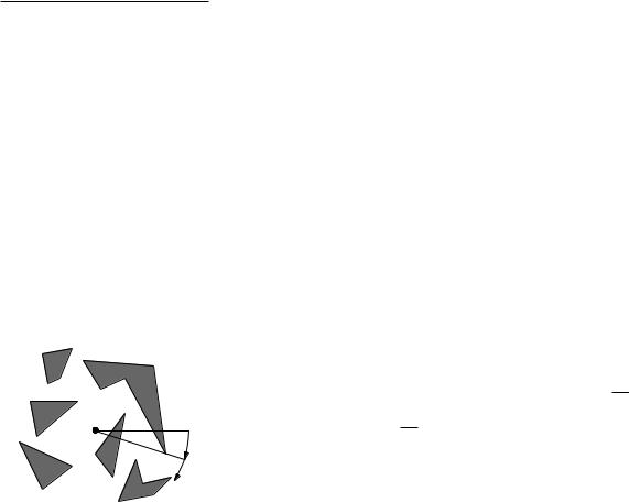
to eν (with respect to the order along ρ ). Figure 15.3 shows an example. Treating the vertices in cyclic order effectively means that we rotate the

half-line ρ around p. So our approach is similar to the plane sweep paradigm we used at various other places; the difference is that instead of using a horizontal line moving downward to sweep the plane, we use a rotating half-line.

The status of our rotational plane sweep is the ordered sequence of obstacle edges intersected by ρ . It is maintained in T. The events in the sweep are the vertices of S. To deal with a vertex w we have to decide whether w is visible from p by searching in the status structure T, and we have to update T by inserting and/or deleting the obstacle edges incident to w.

Algorithm VISIBLEVERTICES summarizes our rotational plane sweep. The sweep is started with the half-line ρ pointing into the positive x-direction and proceeds in clockwise direction. So the algorithm first sorts the vertices by the clockwise angle that the segment from p to each vertex makes with the positive x-axis. What do we do if this angle is equal for two or more vertices? To be able to decide on the visibility of a vertex w, we need to know whether pw intersects

ρthe interior of any obstacle. Hence, the obvious choice is to treat any vertices

that may lie in the interior of pw before we treat w. In other words, vertices for which the angle is the same are treated in order of increasing distance to p. The algorithm now becomes as follows:


Algorithm VISIBLEVERTICES(p, S)


Input. A set S of polygonal obstacles and a point p that does not lie in the


interior of any obstacle.


Output. The set of all obstacle vertices visible from p.


1.

Sort the obstacle vertices according to the clockwise angle that the half-


line from p to each vertex makes with the positive x-axis. In case of


ties, vertices closer to p should come before vertices farther from p. Let


w1, . . . , wn be the sorted list.


2.

Let ρ be the half-line parallel to the positive x-axis starting at p. Find


the obstacle edges that are properly intersected by ρ , and store them in a


balanced search tree T in the order in which they are intersected by ρ .


3.

W ← 0/


4.

for i ← 1 to n


5.

do if VISIBLE(wi) then Add wi to W .


6.

Insert into T the obstacle edges incident to wi that lie on the clock-


wise side of the half-line from p to wi.


7.

Delete from T the obstacle edges incident to wi that lie on the


counterclockwise side of the half-line from p to wi.


328

8.

return W

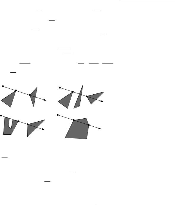
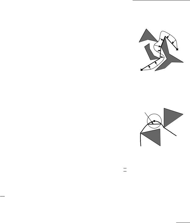
The subroutine VISIBLE must decide whether a vertex wi is visible. Normally, this only involves searching in T to see if the edge closest to p, which is stored in the leftmost leaf, intersects pwi. But we have to be careful when pwi contains other vertices. Is wi visible or not in such a case? That depends. See Figure 15.4 for some of the cases that can occur. pwi may or may not intersect the interior of the obstacles incident to these vertices. It seems that we have to inspect all edges with a vertex on pwi to decide if wi is visible. Fortunately we have already inspected them while treating the preceding vertices that lie on pwi. We can therefore decide on the visibility of wi as follows. If wi−1 is not visible then wi is not visible either. If wi−1 is visible then there are two ways in which wi can be invisible. Either the whole segment wi−1wi lies in an obstacle of which both wi−1 and wi are vertices, or the segment wi−1wi is intersected by an edge in T. (Because in the latter case this edge lies between wi−1 and wi, it must properly intersect wi−1wi.) This test is correct because pwi = pwi−1 wi−1wi. (If i = 1, then there is no vertex in between p and wi, so we only have to look at the segment pwi.) We get the following subroutine:

Section 15.2

COMPUTING THE VISIBILITY GRAPH

p


p


wi−1


wi 1


wi

wi


p


p

Figure 15.4

wi 1


wi−1


wi

Some examples where ρ contains


wi

multiple vertices. In all these cases


wi−1 is visible. In the left two cases wi


is also visible and in the right two cases


wi is not visible.

VISIBLE(wi)

1.if pwi intersects the interior of the obstacle of which wi is a vertex, locally at wi

2.then return false

3.else if i = 1 or wi−1 is not on the segment pwi

4.then Search in T for the edge e in the leftmost leaf.

5.

if e exists and

pwi

intersects e

6.

then return false

7.

else return true

8.else if wi−1 is not visible

9.

then return false


10.

else Search in T for an edge e that intersects

wi−1wi

.


11.

if e exists


12.

then return false


13.

else return true

329

Chapter 15

VISIBILITY GRAPHS

This finishes the description of the algorithm VISIBLEVERTICES to compute the vertices visible from a given point p.

What is the running time of VISIBLEVERTICES? The time we spent before line 4 is dominated by the time to sort the vertices in cyclic order around p, which is O(n log n). Each execution of the loop involves a constant number of operations on the balanced search tree T, which take O(log n) time, plus a constant number of geometric tests that take constant time. Hence, one execution takes O(log n) time, leading to an overall running time of O(n log n).

Recall that we have to apply VISIBLEVERTICES to each of the n vertices of S in order to compute the entire visibility graph. We get the following theorem:

Theorem 15.4 The visibility graph of a set S of disjoint polygonal obstacles with n edges in total can be computed in O(n2 log n) time.

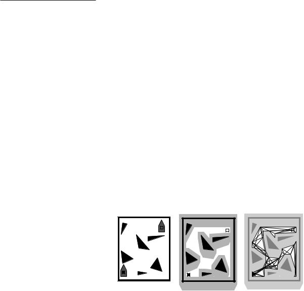
15.3Shortest Paths for a Translating Polygonal Robot

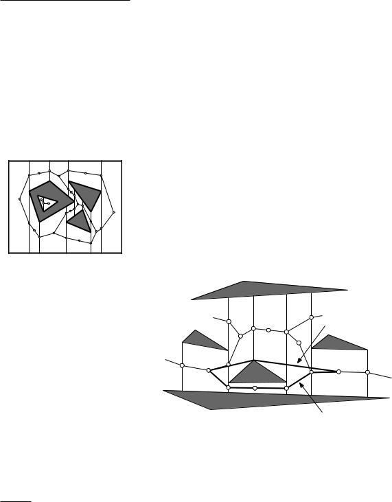
In Chapter 13 we have seen that we can reduce the motion planning problem for a translating, convex, polygonal robot R to the case of a point robot by computing the free configuration space Cfree. The reduction involves computing the Minkowski sum of R, a reflected copy of R, with each of the obstacles, and taking the union of the resulting configuration-space obstacles. This gives us a

work space


configuration space


visibility graph


Figure 15.5

Computing a shortest path for a polygonal robot


set of disjoint polygons, whose union is the forbidden configuration space. We


can then compute a shortest path with the method we used for a point robot: we


extend the set of polygons with the points in configuration space that correspond


to the start and goal placement, compute the visibility graph of the polygons,


assign each arc a weight which is the Euclidean length of the corresponding


visibility edge, and find a shortest path in the visibility graph using Dijkstra’s


algorithm.


To what running time does this approach lead? Lemma 13.13 states that


the forbidden space can be computed in O(n log2 n) time. Furthermore, the

330

complexity of the forbidden space is O(n) by Theorem 13.12, so from the

previous section we know that the visibility graph of the forbidden space can be computed in O(n2 log n) time.

This leads to the following result:

Theorem 15.5 Let R be a convex, constant-complexity robot that can translate among a set of polygonal obstacles with n edges in total. A shortest collisionfree path for R from a given start placement to a given goal placement can be computed in O(n2 log n) time.

Section 15.4

NOTES AND COMMENTS

15.4 Notes and Comments

The problem of computing the shortest path in a weighted graph has been studied extensively. Dijkstra’s algorithm and other solutions are described in most books on graph algorithms and in many books on algorithms and data structures. In Section 15.1 we stated that Dijkstra’s algorithm runs in O(n log n + k) time. To achieve this time bound, one has to use Fibonacci heaps in the implementation. In our application an O((n + k) log n) algorithm would also do fine, since the rest of the algorithm needs that much time anyway.

The geometric version of the shortest path problem has also received consid-


erable attention. The algorithm given here is due to Lee [247]. More efficient


algorithms based on arrangements have been proposed; they run in O(n2)


time [23, 158, 383].


Any algorithm that computes a shortest path by first constructing the entire


visibility graph is doomed to have at least quadratic running time in the worst


case, because the visibility graph can have a quadratic number of edges. For a


long time no approaches were known with a subquadratic worst-case running


time. Mitchell [281] was the first to break the quadratic barrier: he showed that


the shortest path for a point robot can be computed in O(n5/3+ε ) time. Later he


improved the running time of his algorithm to O(n3/2+ε ) [282]. In the mean


time, however, Hershberger and Suri [210, 212] succeeded in developing an


optimal O(n log n) time algorithm.


In the special case where the free space of the robot is a polygon without


holes, a shortest path can be computed in linear time by combining the linear-


time triangulation algorithm of Chazelle [94] with the shortest path method of


Guibas et al. [195].


The 3-dimensional version of the Euclidean shortest path problem is much


harder. This is due to the fact that there is no easy way to discretize the problem:


the inflection points of the shortest path are not restricted to a finite set of points,


but they can lie anywhere on the obstacle edges. Canny [80] proved that the


problem of computing a shortest path connecting two points among polyhedral


obstacles in 3-dimensional space is NP-hard. Reif and Storer [327] gave a single-


exponential algorithm for the problem, by reducing it to a decision problem


in the theory of real numbers. There are also several papers that approximate


the shortest path in polynomial time, for example, by adding points on obstacle


edges and searching a graph with these points as nodes [13, 125, 126, 260, 316].

331

Chapter 15

VISIBILITY GRAPHS

In this chapter we concentrated on the Euclidean metric. Various papers deal with shortest paths under a different metric. Because the number of settings is quite large, we mention only a few, and we give only a few references for each setting. An interesting metric that has been studied is the link metric, where the length of a polygonal path is the number of links it consists of [20, 122, 284, 367]. Another case that has been studied extensively is that of rectilinear paths. Such paths play an important role in VLSI design, for instance. Lee et al. [253] give a survey of rectilinear path problems. An interesting metric that has been studied for rectilinear paths is the combined metric, which is a linear combination of the Euclidean metric and the link metric [56]. Finally, there are papers that consider paths in a subdivision where each region has a weight associated with it. The cost of a path through a region is then its Euclidean length times the weight of the region. Obstacles can be modeled by regions with infinite weight [113, 283].

While there are many obvious metrics for translating robots—in particular, the Euclidean metric immediately comes to mind—it is not so easy to give a good definition of a shortest path for a robot that can rotate as well as translate. Some results have been obtained for the case where the robot is a line segment [24, 114, 218].

The visibility graph was introduced for planning motions by Nilson [295]. The O(n2 log n) time algorithm that we described to compute it is due to Lee [247]. A number of faster algorithms are known [23, 383], including an optimal algorithm by Ghosh and Mount [190], which runs in O(n log n + k) time, where k is the number of arcs of the visibility graph.

To compute a shortest path for a point robot among a set of convex polygonal obstacles, one does not need all the visibility edges. One only needs the visibility edges that define a common tangent. Rohnert [329] gave an algorithm that computes this reduced visibility graph in time O(n + c2 log n), where c is the number of obstacles, and n is their total number of edges.

The visibility complex, introduced by Vegter and Pocchiola [319, 320, 376] is a structure that has the same complexity as the visibility graph, but contains more information. It is defined on a set of convex (not necessarily polygonal) objects in the plane, and can be used for shortest path problems and ray shooting. It can be computed in O(n log n + k) time. Wein et al. [382] introduced an interesting variant of this, the visibility–Voronoi complex, which combines the visibility complex with the Voronoi diagram of the obstacles. This allows one to find short paths that do not come too close to the obstacles.

15.5

Exercises


15.1 Let S be a set of disjoint simple polygons in the plane with n edges in


total. Prove that for any start and goal position the number of segments


on the shortest path is bounded by O(n). Give an example where it

332


is Θ(n).

15.2Algorithm VISIBILITYGRAPH calls algorithm VISIBLEVERTICES with each obstacle vertex. VISIBLEVERTICES sorts all vertices around its

input point. This means that n cyclic sortings are done, one around each obstacle vertex. In this chapter we simply did every sort in O(n log n) time, leading to O(n2 log n) time for all sortings. Show that this can be improved to O(n2) time using dualization (see Chapter 8). Does this improve the running time of VISIBILITYGRAPH?

15.3The algorithm for finding the shortest path can be extended to objects other than polygons. Let S be a set of n disjoint disc-shaped obstacles, not necessarily of equal radius.

a.Prove that in this case the shortest path between two points not seeing each other consists of parts of boundaries of the discs, and/or common tangents of discs, and/or tangents from the start or goal point to the discs.

b.Adapt the notion of a visibility graph for this situation.

c.Adapt the shortest path algorithm to find the shortest path between two points among the discs in S.

15.4What is the maximal number of shortest paths connecting two fixed points among a set of n triangles in the plane?

15.5Let S be a set of disjoint polygons and let a starting point pstart be given. We want to preprocess the set S (and pstart) such that for different goal

points we can efficiently find the shortest path from pstart to the goal. Describe how the preprocessing can be done in time O(n2 log n) such

that for any given goal point pgoal we can compute the shortest path from pstart to pgoal in time O(n log n).

15.6Design an algorithm to find a shortest paths between two points inside a simple polygon. Your algorithm should run in subquadratic time.

15.7When all obstacles are convex polygons we can improve the shortest path algorithm by only considering common tangents rather than all visibility edges.

a.Prove that the only visibility edges that are required in the shortest path algorithm are the common tangents of the polygons.

b.Give a fast algorithm to find the common tangents of two disjoint convex polygons.

c.Give an algorithm to compute those common tangents that are also visibility edges among a set of convex polygons.

15.8* If you are familiar with homogeneous coordinates, it is interesting to see that the rotational sweep that we used in this chapter can be transformed into a normal plane sweep using a horizontal line that translates over the plane. Show that this is the case using a projective transformation that moves the center of the sweep to a point at infinity.

Section 15.5

EXERCISES

333