

- •Preface
- •Contents
- •1 Computational Geometry
- •2 Line Segment Intersection
- •3 Polygon Triangulation
- •4 Linear Programming
- •5 Orthogonal Range Searching
- •6 Point Location
- •7 Voronoi Diagrams
- •8 Arrangements and Duality
- •9 Delaunay Triangulations
- •10 More Geometric Data Structures
- •11 Convex Hulls
- •12 Binary Space Partitions
- •13 Robot Motion Planning
- •14 Quadtrees
- •15 Visibility Graphs
- •16 Simplex Range Searching
- •Bibliography
- •Index

12 Binary Space Partitions
The Painter’s Algorithm
These days pilots no longer have their first flying experience in the air, but on the ground in a flight simulator. This is cheaper for the air company, safer for the pilot, and better for the environment. Only after spending many hours in the simulator are pilots allowed to operate the control stick of a real airplane. Flight simulators must perform many different tasks to make the pilot forget that she is sitting in a simulator. An important task is visualization: pilots must be able to see the landscape above which they are flying, or the runway on which they are landing. This involves both modeling landscapes and rendering the models. To render a scene we must determine for each pixel on the screen the object that is visible at that pixel; this is called hidden surface removal. We must also perform shading calculations, that is, we must compute the intensity of the light that the visible object emits in the direction of the view point. The latter task is very time-consuming if highly realistic images are desired: we must compute how much light reaches the object—either directly from light sources or indirectly via reflections on other objects—and consider the interaction of the light with the surface of the object to see how much of it is reflected in the direction of the view point. In flight simulators rendering must be performed in real-time, so there is no time for accurate shading calculations. Therefore a fast and simple shading technique is employed and hidden surface removal becomes an important factor in the rendering time.
The z-buffer algorithm is a very simple method for hidden surface removal. |
|
This method works as follows. First, the scene is transformed such that the |
|
viewing direction is the positive z-direction. Then the objects in the scene |
|
are scan-converted in arbitrary order. Scan-converting an object amounts to |
|
determining which pixels it covers in the projection; these are the pixels where |
|
the object is potentially visible. The algorithm maintains information about the |
|
already processed objects in two buffers: a frame buffer and a z-buffer. The |
|
frame buffer stores for each pixel the intensity of the currently visible object, |
|
that is, the object that is visible among those already processed. The z-buffer |
|
stores for each pixel the z-coordinate of the currently visible object. (More |
|
precisely, it stores the z-coordinate of the point on the object that is visible at |
|
the pixel.) Now suppose that we select a pixel when scan-converting an object. |
259 |
Chapter 12
BINARY SPACE PARTITIONS
If the z-coordinate of the object at that pixel is smaller than the z-coordinate stored in the z-buffer, then the new object lies in front of the currently visible object. So we write the intensity of the new object to the frame buffer, and its z-coordinate to the z-buffer. If the z-coordinate of the object at that pixel is larger than the z-coordinate stored in the z-buffer, then the new object is not visible, and the frame buffer and z-buffer remain unchanged. The z-buffer algorithm is easily implemented in hardware and quite fast in practice. Hence, this is the most popular hidden surface removal method. Nevertheless, the algorithm has
|
Figure 12.1 |
2 |
3 |
|
|
|
|
|
|
|
|||
|
|
|
|
|||
|
|
|
|
|||
|
|
|
|
|||
|
|
|
|
|||
|
|
|
|
|||
|
|
|
|
|||
|
|
|
||||
|
|
|
|
|
|
|
|
|
|
|
|
|
|
|
|
|
|
|
|
|
|
|
|
|
|
|
|
|
|
|
|
|
|
|
|
|
|
|
|
||
|
|
|
|
|
||
|
|
|
|
|
||
The painter’s algorithm in action |
|
|
|
|
|
|
|
|
|
|
|
||
|
|
|
|
|
||
|
|
some disadvantages: a large amount of extra storage is needed for the z-buffer, |
||||
|
|
and an extra test on the z-coordinate is required for every pixel covered by an |
||||
|
|
object. The painter’s algorithm avoids these extra costs by first sorting the |
||||
|
|
objects according to their distance to the view point. Then the objects are scan- |
||||
|
|
converted in this so-called depth order, starting with the object farthest from |
||||
|
|
the view point. When an object is scan-converted we do not need to perform |
||||
|
|
any test on its z-coordinate, we always write its intensity to the frame buffer. |
||||
|
|
Entries in the frame buffer that have been filled before are simply overwritten. |
||||
|
|
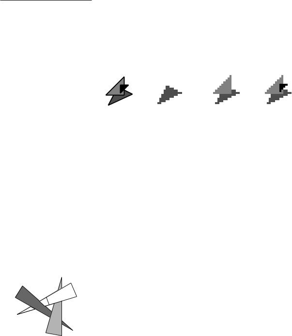
Figure 12.1 illustrates the algorithm on a scene consisting of three triangles. |
||||
|
|
On the left, the triangles are shown with numbers corresponding to the order |
||||
|
|
in which they are scan-converted. The images after the first, second, and third |
||||
|
|
triangle have been scan-converted are shown as well. This approach is correct |
||||
|
|
because we scan-convert the objects in back-to-front order: for each pixel the |
||||
|
|
last object written to the corresponding entry in the frame buffer will be the one |
||||
|
|
closest to the viewpoint, resulting in a correct view of the scene. The process |
||||
|
|
resembles the way painters work when they put layers of paint on top of each |
||||
|
|
other, hence the name of the algorithm. |
||||
|
|
To apply this method successfully we must be able to sort the objects quickly. |
||||
|
|
Unfortunately this is not so easy. Even worse, a depth order may not always |
||||
|
|
exist: the in-front-of relation among the objects can contain cycles. When such |
||||
|
|
a cyclic overlap occurs, no ordering will produce a correct view of this scene. In |
||||
|
|
this case we must break the cycles by splitting one or more of the objects, and |
||||
|
|
hope that a depth order exists for the pieces that result from the splitting. When |
||||
|
|
there is a cycle of three triangles, for instance, we can always split one of them |
||||
|
|
into a triangular piece and a quadrilateral piece, such that a correct displaying |
||||
|
|
order exists for the resulting set of four objects. Computing which objects to |
||||
|
|
split, where to split them, and then sorting the object fragments is an expensive |
||||
|
|
process. Because the order depends on the position of the view point, we must |
||||
|
|
recompute the order every time the view point moves. If we want to use the |
||||
|
|
painter’s algorithm in a real-time environment such as flight simulation, we |
||||
260 |
|
should preprocess the scene such that a correct displaying order can be found |
||||
quickly for any view point. An elegant data structure that makes this possible is |
Section 12.1 |
the binary space partition tree, or BSP tree for short. |
THE DEFINITION OF BSP TREES |
12.1The Definition of BSP Trees
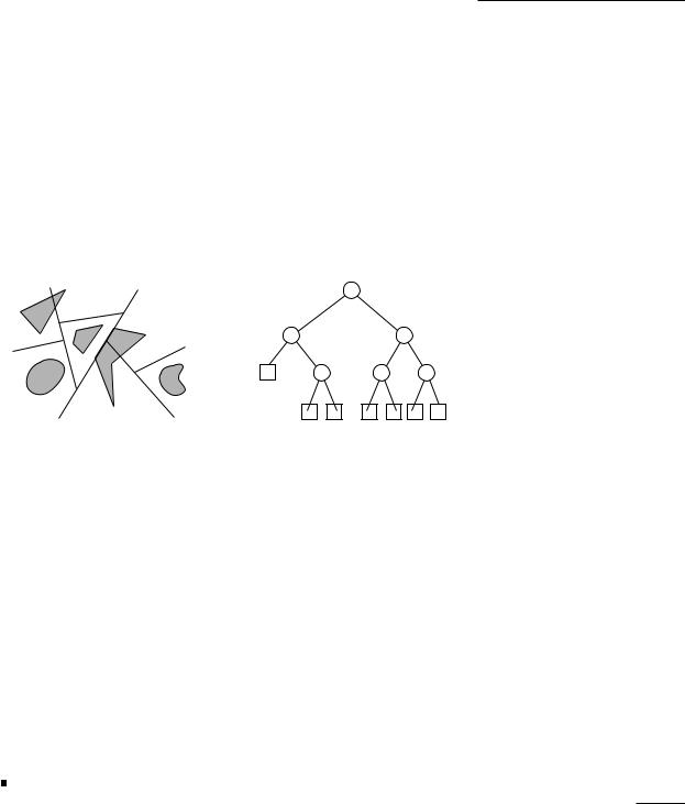
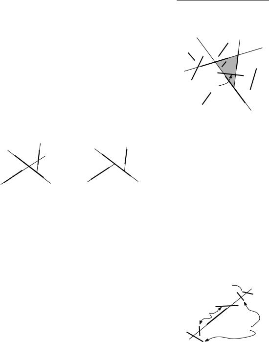
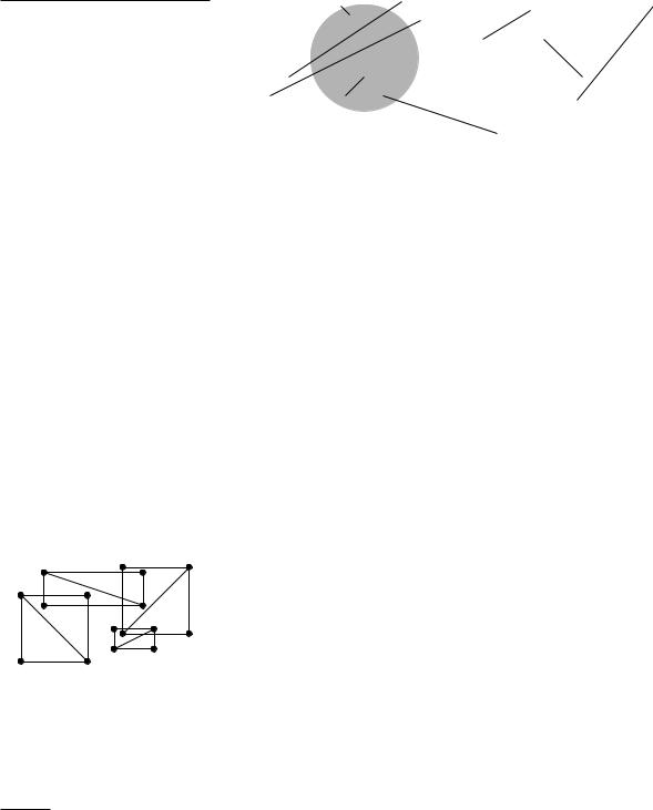
To get a feeling for what a BSP tree is, take a look at Figure 12.2. This figure shows a binary space partition (BSP) for a set of objects in the plane, together with the tree that corresponds to the BSP. As you can see, the binary space partition is obtained by recursively splitting the plane with a line: first we split the entire plane with 1, then we split the half-plane above 1 with 2 and the half-plane below 1 with 3, and so on. The splitting lines not only partition the plane, they may also cut objects into fragments. The splitting continues until there is only one fragment left in the interior of each region. This process is
2 |
1 |
o1 4
|
5 |
o3 |
o4 |
|
6 |
3 |
|
|
|
|
|
||
|
o |
2 |
|
o5 |
o4 |
|
|
|
|
|
6 |
1 |
2 |
5 |
4 |
3 |
o5 |
|
o4 |
|
o2 |
|
o1 |
|
o1 |
o3 |
|
|
|
|
|
|
|
|
|
|
Figure 12.2
A binary space partition and the corresponding tree
naturally modeled as a binary tree. Each leaf of this tree corresponds to a face of the final subdivision; the object fragment that lies in the face is stored at the leaf. Each internal node corresponds to a splitting line; this line is stored at the node. When there are 1-dimensional objects (line segments) in the scene then objects could be contained in a splitting line; in that case the corresponding internal node stores these objects in a list.
For a hyperplane h : a1x1 + a2x2 + ···+ ad xd + ad+1 = 0, we let h+ be the open positive half-space bounded by h and we let h− be the open negative half-space:
h+ := {(x1, x2, . . . , xd ) : a1x1 + a2x2 + ···+ ad xd + ad+1 > 0} |
|
and |
|
h− := {(x1, x2, . . . , xd ) : a1x1 + a2x2 + ···+ ad xd + ad+1 < 0}. |
|
A binary space partition tree, or BSP tree, for a set S of objects in d-dimensional |
|
space is now defined as a binary tree T with the following properties: |
|
If card(S) 1 then T is a leaf; the object fragment in S (if it exists) is stored |
|
explicitly at this leaf. If the leaf is denoted by ν , then the (possibly empty) |
|
set stored at the leaf is denoted by S(ν ). |
261 |
Chapter 12
BINARY SPACE PARTITIONS
If card(S) > 1 then the root ν of T stores a hyperplane hν , together with the set S(ν ) of objects that are fully contained in hν . The left child of ν is the root of a BSP tree T− for the set S− := {h−ν ∩s : s S}, and the right child of ν is the root of a BSP tree T+ for the set S+ := {h+ν ∩s : s S}.
The size of a BSP tree is the total size of the sets S(ν ) over all nodes ν of the BSP tree. In other words, the size of a BSP tree is the total number of object fragments that are generated. If the BSP does not contain useless splitting lines—lines that split off an empty subspace—then the number of nodes of the tree is at most linear in the size of the BSP tree. Strictly speaking, the size of the BSP tree does not say anything about the amount of storage needed to store it, because it says nothing about the amount of storage needed for a single fragment. Nevertheless, the size of a BSP tree as we defined it is a good measure to compare the quality of different BSP trees for a given set of objects.
2 |
1 |
|
|
|
1 |
|
3 |
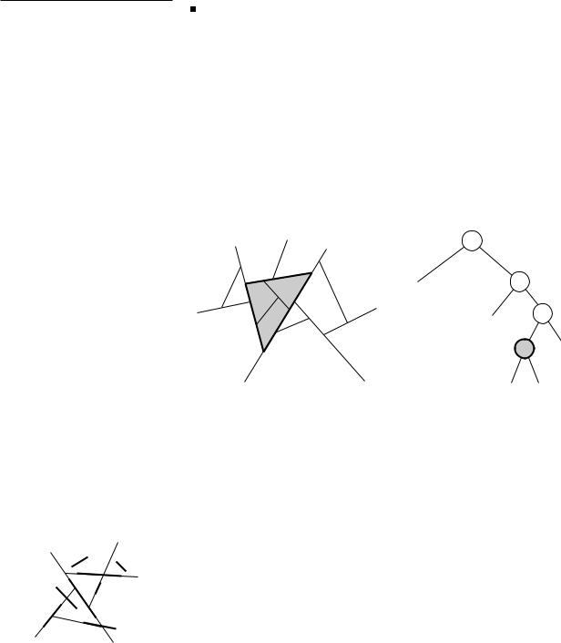
Figure 12.3
The correspondence between nodes and regions
2 |
3 |
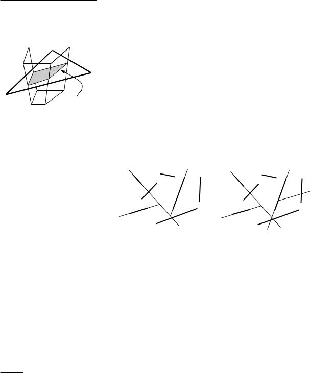
The leaves in a BSP tree represent the faces in the subdivision that the BSP induces. More generally, we can identify a convex region with each node ν in a BSP tree T: this region is the intersection of the half-spaces hµ , where µ is an ancestor of ν and = − when ν is in the left subtree of µ , and = + when it is in the right subtree. The region corresponding to the root of T is the whole space. Figure 12.3 illustrates this: the grey node corresponds to the grey region
|
1+ ∩ 2+ ∩ 3−. |
|
The splitting hyperplanes used in a BSP can be arbitrary. For computational |
|
purposes, however, it can be convenient to restrict the set of allowable splitting |
|
hyperplanes. A usual restriction is the following. Suppose we want to construct |
|
a BSP for a set of line segments in the plane. An obvious set of candidates for |
|
the splitting lines is the set of extensions of the input segments. A BSP that only |
|
uses such splitting lines is called an auto-partition. For a set of planar polygons |
|
in 3-space, an auto-partition is a BSP that only uses planes through the input |
|
polygons as splitting planes. It seems that the restriction to auto-partitions is a |
|
severe one. But, although auto-partitions cannot always produce minimum-size |
262 |
BSP trees, we shall see that they can produce reasonably small ones. |
12.2BSP Trees and the Painter’s Algorithm
Suppose we have built a BSP tree T on a set S of objects in 3-dimensional space. How can we use T to get the depth order we need to display the set S with the painter’s algorithm? Let pview be the view point and suppose that pview lies above the splitting plane stored at the root of T. Then clearly none of the objects below the splitting plane can obscure any of the objects above it. Hence, we can safely display all the objects (more precisely, object fragments) in the subtree T− before displaying those in T+. The order for the object fragments in the two subtrees T+ and T− is obtained recursively in the same way. This is summarized in the following algorithm.
Algorithm PAINTERSALGORITHM(T, pview)
1.Let ν be the root of T.
2.if ν is a leaf
3.then Scan-convert the object fragments in S(ν ).
4.else if pview h+ν
5.then PAINTERSALGORITHM(T−, pview)
6. |
Scan-convert the object fragments in S(ν ). |
7. |
PAINTERSALGORITHM(T+, pview) |
8.else if pview h−ν
9. |
then PAINTERSALGORITHM(T+, pview) |
||
10. |
Scan-convert the object fragments in S(ν ). |
||
11. |
PAINTERSALGORITHM(T−, pview) |
||
12. |
else ( pview hν ) |
+ |
, pview) |
13. |
PAINTERSALGORITHM(T |
|
|
14. |
PAINTERSALGORITHM(T−, pview) |
||
Note that we do not draw the polygons in S(ν ) when pview lies on the splitting plane hν , because polygons are flat 2-dimensional objects and therefore not visible from points that lie in the plane containing them.
The efficiency of this algorithm—indeed, of any algorithm that uses BSP trees— depends largely on the size of the BSP tree. So we must choose the splitting planes in such a way that fragmentation of the objects is kept to a minimum. Before we can develop splitting strategies that produce small BSP trees, we must decide on which types of objects we allow. We became interested in BSP trees because we needed a fast way of doing hidden surface removal for flight simulators. Because speed is our main concern, we should keep the type of objects in the scene simple: we should not use curved surfaces, but represent everything in a polyhedral model. We assume that the facets of the polyhedra have been triangulated. So we want to construct a BSP tree of small size for a given set of triangles in 3-dimensional space.
Section 12.2
BSP TREES AND THE PAINTER’S
ALGORITHM
h+ν
h−ν
hν
263

Chapter 12
BINARY SPACE PARTITIONS
(s)
s
264
12.3Constructing a BSP Tree
When you want to solve a 3-dimensional problem, it is usually not a bad idea to gain some insight by first studying the planar version of the problem. This is also what we do in this section.
Let S be a set of n non-intersecting line segments in the plane. We will restrict our attention to auto-partitions, that is, we only consider lines containing one of the segments in S as candidate splitting lines. The following recursive algorithm for constructing a BSP immediately suggests itself. Let (s) denote the line that contains a segment s.
Algorithm 2DBSP(S)
Input. A set S = {s1, s2, . . . , sn} of segments.
Output. A BSP tree for S.
1.if card(S) 1
2.then Create a tree T consisting of a single leaf node, where the set S is
stored explicitly.
3. |
return T |
) |
|
|
|
|
|
|
|
|
|
4. |
else ( +Use |
(s |
the splitting line. |
) |
+ |
|
|||||
1 |
|
as |
+ |
: s S}; |
|
+ |
←2DBSP(S |
|
|||
5. |
S ← {s ∩ (s1) |
|
T |
|
|
) |
|||||
6. |
S− ← {s ∩ (s1)− : s S}; |
T− ←2DBSP(S−) |
|||||||||
7.Create a BSP tree T with root node ν , left subtree T−, right subtree T+, and with S(ν ) = {s S : s (s1)}.
8.return T
The algorithm clearly constructs a BSP tree for the set S. But is it a small one? Perhaps we should spend a little more effort in choosing the right segment to do the splitting, instead of blindly taking the first segment, s1. One approach that comes to mind is to take the segment s S such that (s) cuts as few segments as possible. But this is too greedy: there are configurations of segments where this approach doesn’t work well. Furthermore, finding this segment would be time consuming. What else can we do? Perhaps you already guessed: as in previous chapters where we had to make a difficult choice, we simply make a random choice. That is to say, we use a random segment to do the splitting. As we shall see later, the resulting BSP is expected to be fairly small.
To implement this, we put the segments in random order before we start the construction:
Algorithm 2DRANDOMBSP(S)
1.Generate a random permutation S = s1, . . . , sn of the set S.
2.T ←2DBSP(S )
3.return T
Before we analyze this randomized algorithm, we note that one simple optimization is possible. Suppose that we have chosen the first few partition lines. These lines induce a subdivision of the plane whose faces correspond to nodes in the BSP tree that we are constructing. Consider one such face f . There can
be segments that cross f completely. Selecting one of these crossing segments to split f will not cause any fragmentation of other segments inside f , while the segment itself can be excluded from further consideration. It would be foolish not to take advantage of such free splits. So our improved strategy is to make free splits whenever possible, and to use random splits otherwise. To implement this optimization, we must be able to tell whether a segment is a free split. To this end we maintain two boolean variables with each segment, which indicate whether the left and right endpoint lie on one of the already added splitting lines. When both variables become true, then the segment is a free split.
We now analyze the performance of algorithm 2DRANDOMBSP. To keep it simple, we will analyze the version without free splits. (In fact, free splits do not make a difference asympotically.)
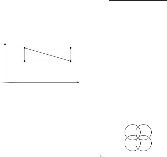
We start by analyzing the size of the BSP tree or, in other words, the number of fragments that are generated. Of course, this number depends heavily on the particular permutation generated in line 1: some permutations may give small BSP trees, while others give very large ones. As an example, consider the
Section 12.3
CONSTRUCTING A BSP TREE
f
free split
(a) |
s3 |
(b) |
|
|
|
s2 |
s1 |
s3 |
|
|
s1 |
s2 |
|
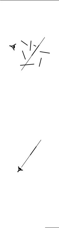
Figure 12.4 |
|
|
Different orders give different BSPs |
||
|
|
|
||
collection of three segments depicted in Figure 12.4. If the segments are treated |
|
|||
as illustrated in part (a) of the figure, then five fragments result. A different |
|
|||
order, however, gives only three fragments, as shown in part (b). Because the |
|
|||
size of the BSP varies with the permutation that is used, we will analyze the |
|
|||
expected size of the BSP tree, that is, the average size over all n! permutations. |
|
|||
Lemma 12.1 The expected number of fragments generated by the algorithm |
|
|||
2DRANDOMBSP is O(n log n). |
|
|
|
|
Proof. Let si be a fixed segment in S. We shall analyze the expected number |
|
|||
of other segments that are cut when (si) is added by the algorithm as the next |
|
|||
splitting line. |
|
|
is cut when (si) |
dist= 2 |
In Figure 12.4 we can see that whether or not a segment s j |
||||
is added—assuming it can be cut at all by (si)—depends on segments that are |
|
|||
also cut by (si) and are ‘in between’ si and s j. In particular, when the line |
|
|||
through such a segment is used before (si), then it shields s j |
from si. This is |
dist= 0 |
||
what happened in Figure 12.4(b): the segment s1 shielded s3 from s2. These |
si |
|||
considerations lead us to define the distance of a segment with respect to the |
dist= 1 |
|||
fixed segment si: |
|
|
|
|
|
|
|
|
the number of segments intersecting |
if (s |
) intersects s |
|
|
distsi (s j) = |
(si) in between si and s j |
i |
|
j |
||
|
|
|
|
|||
|
|
|
otherwise |
265 |
||
|
+∞ |
|||||
Chapter 12
BINARY SPACE PARTITIONS
For any finite distance, there are at most two segments at that distance, one on either side of si.
Let k := distsi (s j), and let s j1 , s j2 , . . . , s jk be the segments in between si and s j. What is the probability that (si) cuts s j when added as a splitting line?
For this to happen, si must come before s j in the random ordering and, moreover, it must come before any of the segments in between si and s j, which shield s j from si. In other words, of the set {i, j, j1, . . . , jk} of indices, i must be the smallest one. Because the order of the segments is random, this implies
1 Pr[ (si) cuts s j] distsi (s j) + 2 .
Notice that there can be segments that are not cut by (si) but whose extension shields s j. This explains why the expression above is not an equality.
We can now bound the expected total number of cuts generated by si:
E[number of cuts generated by si] |
∑ |
|
1 |
|
|
distsi (s j) + 2 |
|||||
|
|
||||
|
j =i |
|
|
||
|
n−2 |
1 |
|
||
|
2 ∑ |
|
|
||
k + 2 |
|||||
|
k=0 |
||||
|
|
|
|||
2 ln n. |
|||||
By linearity of expectation, we can conclude that the expected total number of cuts generated by all segments is at most 2n ln n. Since we start with n segments, the expected total number of fragments is bounded by n + 2n ln n. 


We have shown that the expected size of the BSP that is generated by 2DRANDOMBSP is n + 2n ln n. As a consequence, we have proven that a BSP of size n + 2n ln n exists for any set of n segments. Furthermore, at least half of all permutations lead to a BSP of size n + 4n ln n. We can use this to find a BSP of that size: After running 2DRANDOMBSP we test the size of the tree, and if it exceeds that bound, we simply start the algorithm again with a fresh random
|
permutation. The expected number of trials is two. |
|
We have analyzed the size of the BSP that is produced by 2DRANDOMBSP. |
|
What about the running time? Again, this depends on the random permutation |
|
that is used, so we look at the expected running time. Computing the random |
|
permutation takes linear time. If we ignore the time for the recursive calls, |
|
then the time taken by algorithm 2DBSP is linear in the number of fragments |
|
in S. This number is never larger than n—in fact, it gets smaller with each |
|
recursive call. Finally, the number of recursive calls is obviously bounded by |
|
the total number of generated fragments, which is O(n log n). Hence, the total |
|
construction time is O(n2 log n), and we get the following result. |
|
Theorem 12.2 A BSP of size O(n log n) can be computed in expected time |
266 |
O(n2 log n). |

Although the expected size of the BSP that is constructed by 2DRAN- DOMBSP is fairly good, the running time of the algorithm is somewhat disappointing. In many applications this is not so important, because the construction is done off-line. Moreover, the construction time is only quadratic when the BSP is very unbalanced, which is rather unlikely to occur in practice. Nevertheless, from a theoretical point of view the construction time is disappointing. Using an approach based on segment trees—see Chapter 10—this can be improved: one can construct a BSP of size O(n log n) in O(n log n) time with a deterministic algorithm. This approach does not give an auto-partition, however, and in practice it produces BSPs that are slightly larger.
A natural question is whether the size of the BSP generated by 2DRAN- DOMBSP can be improved. Would it for example be possible te devise an algorithm that produces a BSP of size O(n) for any set of n disjoint segments in the plane? The answer is no: there are sets of segments for which any BSP must have size Ω(n log n/ log log n). Note that the algorithm we presented does not achieve this bound, so there may still be room for a slight improvement.
The algorithm we described for the planar case generalizes to 3-dimensional space. Let S be a set of n non-intersecting triangles in R3. Again we restrict ourselves to auto-partitions, that is, we only use partition planes containing a triangle of S. For a triangle t we denote the plane containing it by h(t).
Algorithm 3DBSP(S)
Input. A set S = {t1, t2, . . . , tn} of triangles in R3.
Output. A BSP tree for S.
1.if card(S) 1
2.then Create a tree T consisting of a single leaf node, where the set S is
stored explicitly.
3. |
else |
return T |
) |
as + |
+ |
|
+ |
||
4. |
( |
+ |
1 |
) |
|||||
|
|
Use h(t |
the splitting plane. |
|
|||||
5. |
|
S ← {t ∩h(t1) : t S}; |
T ←3DBSP(S ) |
||||||
6. |
|
S− ← {t ∩h(t1)− : t S}; |
T− ←3DBSP(S−) |
||||||
7.Create a BSP tree T with root node ν , left subtree T−, right subtree T+, and with S(ν ) = {t S : t h(t1)}.
8.return T
The size of the resulting BSP again depends on the order of the triangles; some orders give more fragments than others. As in the planar case, we can try to get a good expected size by first putting the triangles in a random order. This usually gives a good result in practice. However, it is not known how to analyze the expected behavior of this algorithm theoretically. Therefore we will analyze a variant of the algorithm in the next section, although the algorithm described above is probably superior in practice.
Section 12.3
CONSTRUCTING A BSP TREE
t
h(t)
267
Chapter 12
BINARY SPACE PARTITIONS
free split
Figure 12.5
The original and the modified algorithm
268
12.4* The Size of BSP Trees in 3-Space
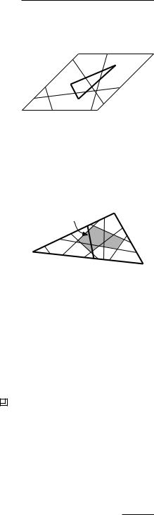
The randomized algorithm for constructing a BSP tree in 3-space that we analyze in this section is almost the same as the improved algorithm described above: it treats the triangles in random order, and it makes free splits whenever possible. A free split now occurs when a triangle of S splits a cell into two disconnected subcells. The only difference is that when we use some plane h(t) as a splitting plane, we use it in all cells intersected by that plane, not just in the cells that are intersected by t. (And therefore a simple recursive implementation is no longer possible.) There is one exception to the rule that we split all cells with h(t): when the split is completely useless for a cell, because all the triangles in that cell lie completely to one side of it, then we do not split it.
Figure 12.5 illustrates this on a 2-dimensional example. In part (a) of the figure, the subdivision is shown that is generated by the algorithm of the previous section after treating segments s1, s2, and s3 (in that order). In part (b) the subdivision is shown as generated by the modified algorithm. Note that the modified algorithm uses (s2) as a splitting line in the subspace below (s1), and that (s3) is used as a splitting line in the subspace to the right of (s2). The line (s3) is not used in the subspace between (s1) and (s2), however, because it is useless there.
(a) |
s1 |
(b) |
s1 |
|
|||
|
s2 |
|
s2 |
|
s3 |
|
s3 |
The modified algorithm can be summarized as follows. Working out the details is left as an exercise.
Algorithm 3DRANDOMBSP2(S)
Input. A set S = {t1, t2, . . . , tn} of triangles in R3.
Output. A BSP tree for S.
1.Generate a random permutation t1, . . . , tn of the set S.
2.for i ← 1 to n
3.do Use h(ti) to split every cell where the split is useful.
4.Make all possible free splits.
The next lemma analyzes the expected number of fragments generated by the algorithm.
Lemma 12.3 The expected number of object fragments generated by algorithm 3DRANDOMBSP2 over all n! possible permutations is O(n2).
Proof. We shall prove a bound on the expected number of fragments into which a fixed triangle tk S is cut. For a triangle ti with i < k we define
i := h(ti) ∩ h(tk). The set L := { 1, . . . , k−1} is a set of at most k − 1 lines lying in the plane h(tk). Some of these lines intersect tk, others miss tk. For
a line i that intersects tk we define si := i ∩tk. Let I be the set of all such intersections si. Due to free splits the number of fragments into which tk is cut is in general not simply the number of faces in the arrangement that I induces on tk. To understand this, consider the moment that tk−1 is treated. Assume thatk−1 intersects tk; otherwise tk−1 does not cause any fragmentation on tk. The segment sk−1 can intersect several of the faces of the arrangement on tk induced by I \{sk}. If, however, such a face f is not incident to the one of the edges of tk—we call f an interior face—then a free split already has been made through this part of tk. In other words, h(tk−1) only causes cuts in exterior faces, that is, faces that are incident to one of the three edges of tk. Hence, the number of splits on tk caused by h(tk−1) equals the number of edges that sk−1 contributes to exterior faces of the arrangement on tk induced by I. (In the analysis that follows, it is important that the collection of exterior faces is independent of the order in which t1, . . . , tk−1 have been treated. This is not the case for the algorithm in the previous section, which is the reason for the modification.) What is the expected number of such edges? To answer this question we first bound the total number of edges of the exterior faces.
In Chapter 8 we defined the zone of a line in an arrangement of lines in the plane as the set of faces of the arrangement intersected by . You may recall that for an arrangement of m lines the complexity of the zone is O(m). Now let e1, e2, and e3 be the edges of tk and let (ei) be the line through ei, for i = 1, 2, 3. The edges that we are interested in must be in the zone of either (e1), (e2), or (e3) in the arrangement induced by the set L on the plane h(tk). Hence, the total number of edges of exterior faces is O(k).
If the total number of edges of exterior faces is O(k), then the average number of edges lying on a segment si is O(1). Because t1, . . . , tn is a random permutation, so is t1, . . . , tk−1. Hence, the expected number of edges on segment sk−1 is constant, and therefore the expected number of extra fragments on tk caused by h(tk−1) is O(1). The same argument shows that the expected number of fragmentations on tk generated by each of the splitting planes h(t1) through h(tk−2) is constant. This implies that the expected number of fragments into which tk is cut is O(k). The total number of fragments is therefore
n
O( ∑ k) = O(n2).
k=1
The quadratic bound on the expected size of the partitioning generated by 3DRANDOMBSP immediately proves that a BSP tree of quadratic size exists.
You may be a bit disappointed by the bound that we have achieved. A quadratic size BSP tree is not what you are hoping for when you have a set of 10,000 triangles. The following theorem tells us that we cannot hope to prove anything better if we restrict ourselves to auto-partitions.
Lemma 12.4 There are sets of n non-intersecting triangles in 3-space for which any auto-partition has size Ω(n2).
Section 12.4*
THE SIZE OF BSP TREES IN 3-SPACE
3 4
1 tk
2
sk−1
tk
269
Chapter 12
BINARY SPACE PARTITIONS
R2
R1
Proof. Consider a collection of rectangles consisting of a set R1 of rectangles parallel to the xy-plane and a set R2 of rectangles parallel to the yz-plane, as illustrated in the margin. (The example also works with a set of triangles, but with rectangles it is easier to visualize.) Let n1 := card(R1), let n2 := card(R2), and let G(n1, n2) be the minimum size of an auto-partition for such a configuration. We claim that G(n1, n2) = (n1 + 1)(n2 + 1) − 1. The proof is by induction on n1 + n2. The claim is obviously true for G(1, 0) and G(0, 1), so now consider the case where n1 + n2 > 1. Without loss of generality, assume that the auto-partition chooses a rectangle r from the set R1. The plane through r will split all the rectangles in R2. Moreover, the configurations in the two subscenes that must be treated recursively have exactly the same form as the initial configuration. If m denotes the number of rectangles of R1 lying above r, then we have
G(n1, n2) = 1 + G(m, n2) + G(n1 −m −1, n2)
= 1 + ((m + 1)(n2 + 1) −1) + ((n1 −m)(n2 + 1) −1) = (n1 + 1)(n2 + 1) −1.
So perhaps we should not restrict ourselves to auto-partitions. In the lower bound in the proof of Lemma 12.4 the restriction to auto-partitions is definitely a bad idea: we have shown that such a partition necessarily has quadratic size,
|
Figure 12.6 |
|
The general lower bound construction |
|
|
|
|
whereas we can easily get a linear BSP if we first separate the set R1 from the |
|
|
set R2 with a plane parallel to the xz-plane. But even unrestricted partitions fail |
|
|
to give a small BSP for the configuration of Figure 12.6. This configuration is |
|
|
obtained as follows. We start by taking a grid in the plane made up of n/2 lines |
|
|
parallel to the x-axis and n/2 lines parallel to the y-axis. (Instead of the lines we |
|
|
could also take very long and skinny triangles.) We skew these lines a little to |
|
|
get the configuration of Figure 12.6; the lines now lie on a so-called hyperbolic |
|
|
paraboloid. Finally we move the lines parallel to the y-axis slightly upward so |
|
|
that the lines no longer intersect. What we get is the set of lines |
|
|
{y = i, z = ix : 1 i n/2} {x = i, z = iy + ε : 1 i n/2}, |
|
|
where ε is a small positive constant. If ε is sufficiently small then any BSP |
270 |
|
must cut at least one of the four lines that bound a grid cell in the immediate |

neighborhood of that cell. The formal proof of this fact is elementary, but tedious and not very instructive. The idea is to show that the lines are skewed in such a way that no plane fits simultaneously through the four “openings” at its corners. Since there is a quadratic number of grid cells, this will result in Θ(n2) fragments.
Theorem 12.5 For any set of n non-intersecting triangles in R3 a BSP tree of
size O(n2) exists. Moreover, there are configurations for which the size of any BSP is Ω(n2).
Section 12.5
BSP TREES FOR LOW-DENSITY
SCENES
12.5 BSP Trees for Low-Density Scenes
In the previous section, we described an algorithm that constructs a BSP tree for a set of n disjoint triangles in R3. It always produces a BSP tree of size O(n2). We also gave an example of a set of n triangles for which any BSP tree has size Ω(n2). Hence, the O(n2) upper bound is tight in the worst case, and from a
theoretical point of view the problem seems to be solved. The tight quadratic |
|
bound might give you the idea that BSP trees are useless in practice. Fortunately |
|
this is not the case: in many practical situations, BSP trees perform just fine. |
|
Evidently, the theoretical analysis fails to predict the practical performance of |
|
BSP trees. |
|
This is disturbing: based on our theoretical analysis we might have discarded |
|
a structure that is quite useful in practice. The problem is that certain inputs— |
|
the grid-like lower-bound construction, for example—force a BSP to cut may |
|
objects, while other inputs—the ones that usually occur in practice—admit |
|
a BSP that cuts only few objects. We would like our analysis to reflect this: |
|
it should give different bounds for different types of input. This means that |
|
we can no longer do the analysis in terms of the input size, n, only. We must |
|
introduce another parameter, which distinguishes easy inputs from difficult ones. |
|
What are easy inputs? Intuitively, easy inputs are inputs where the objects are |
|
relatively well separated, whereas difficult inputs have many objects packed |
|
closely together. Note that whether or not objects are close to each other is not |
|
a matter of the absolute distance between them, but of the distance relative to |
|
their size; otherwise, scaling the whole scene would lead to different results, |
|
which is undesirable. Therefore we define our parameter, which we will call the |
|
density of a scene, as follows. |
|
Let diam(o) denote the diameter of an object o. The density of a set S of |
|
objects in Rd is defined as the smallest number λ such that the following holds: |
|
any ball B intersects at most λ objects o S such that diam(o) diam(B). |
|
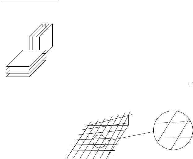
Figure 12.7 illustrates this definition. Note that the definition speaks of any |
|
ball: B is not an object in S, but a ball of arbitrary radius whose center can be |
|
anywhere in space. |
|
It is easy to come up with a set of n objects whose density is n: any set of |
|
lines will do. When the objects are bounded, the density can still be high. The |
|
grid-like construction of Figure 12.6, for example, has density Θ(n) even if the |
|
objects in the construction are line segments rather than full lines. On the other |
271 |
Chapter 12
BINARY SPACE PARTITIONS
Figure 12.7
A set of eight segments with density 3. The disc B intersects five segments, but two of them have diameter less than diam(B) and so they are not counted
272
B
hand, the density can also be quite low: a set of n unit balls such that any two balls are more than unit distance apart has density 1. In fact, one can prove that any set of n disjoint balls has density Θ(1), even if they have vastly different sizes—see Exercise 12.13.
Let’s see where we stand. We have defined a parameter, density, that captures the difficulty of a scene in the following sense: if the density is low then the objects are reasonably well separated, and if the density is high then there are regions with many objects close together. Next we want to show that if the density is low—a constant independent of n, for instance—then we can find a small BSP. One possibility could be to analyze the randomized algorithm of the previous section more carefully, and show that it produces a small BSP if the density of the input set is low. Unfortunately, this is not the case: even for inputs of low density, it may produce a BSP whose expected size is quadratic. In other words, the algorithm fails to always take advantage of the situation when the input scene is easy. We need a new algorithm.
Let S be a set of objects in R2—S can contain segments, discs, triangles, etc.— and let λ be the density of S. (The algorithm presented below also works in R3 and, in fact, even in higher dimensions. For simplicity we shall confine ourselves to R2 from now on.) The idea behind the algorithm is to define, for each object o S, a small set of points—we call them guards—such that the distribution of the guards is representative of the distribution of the objects, and then to let the construction of the BSP be guided by the guards. We shall now make this idea precise.
Let bb(o) denote the bounding box of o, that is, bb(o) is the smallest axisaligned rectangle that contains o. The guards that we define for o are simply the four vertices of bb(o). Let G(S) be the multiset of 4n guards defined for the objects in S. (G(S) is a multiset because bounding-box vertices can coincide. When this happens, we want those guards to be put multiple times into G(S), once for each object of which they are a bounding-box vertex.) When S has low density, the guards in G(S) are representative of the distribution of S in the following sense: for any square σ , the number of objects intersecting σ is not much more than the number of guards inside σ . The next lemma makes this precise. Note that this lemma gives only an upper bound on the number of objects intersecting a square, not a lower bound: it is very well possible that a square contains many guards without intersecting a single object. Note also that even though the definition of density (in 2D) uses discs, the property of the guards given in the following lemma is with respect to squares.
Lemma 12.6 Any axis-parallel square that contains k guards from G(S) in its interior intersects at most k + 4λ objects from S.
Proof. Let σ be an axis-parallel square with k guards in its interior. Obviously there are at most k objects that have a guard (that is, a bounding-box vertex) inside σ . Define S to be the set of the remaining objects from S, that is, the ones without a guard inside σ . Clearly, the density of S is at most λ . We have to show that at most 4λ objects from S can intersect σ .
Section 12.5
BSP TREES FOR LOW-DENSITY
SCENES
y
|
|
|
|
|
|
|
Figure 12.8 |
|||
|
|
|
σ |
|
|
|
The square σ intersects a segment but |
|||
|
|
|
|
|
|
does not contain a guard. Hence, the |
||||
|
|
|
|
|
|
|
||||
|
|
|
|
|
|
|
diameter of the segment is at least the |
|||
|
|
|
|
x |
edge length of σ |
|||||
If an object o S intersects σ then, obviously, bb(o) intersects σ as well. |
|
|
|
|
||||||
By the definition of S , the square σ does not contain a vertex of bb(o) in its |
|
|
|
|
||||||
interior. But then the projection of bb(o) onto the x-axis contains the projection |
|
|
|
|
||||||
of σ onto the x-axis, or the projection of bb(o) onto the y-axis contains the |
|
|
|
|
||||||
projection of σ onto the y-axis (or both)—see Figure 12.8. This implies that the |
|
|
|
|
||||||
diameter of o is at least the side length of σ , and so diam(o) diam(σ )/√ |
|
|
|
|
|
|
||||
2. |
|
|
|
|
||||||
Now cover σ with four discs D1, . . . , D4 of diameter diam(σ )/2. The object o |
|
|
|
|
||||||
intersects at least one of these discs, Di. We charge o to Di. We have |
|
|
|
|
||||||
|
|
|
|
|||||||
diam(o) diam(σ )/√ |
|
> diam(σ )/2 = diam(Di). |
|
|
|
|
||||
2 |
|
|
|
|
||||||
Since S has density at most λ , each Di is charged at most λ times. Hence, σ |
|
|
|
|
||||||
intersects at most 4λ objects from S . Adding the at most k objects not in S , we |
|
|
|
|
||||||
find that σ intersects at most k + 4λ objects from S. |
|
|
|
|
||||||
Lemma 12.6 suggests the following two-phase algorithm to construct a BSP. |
|
|
|
|
||||||
Let U be a square that contains all objects from S in its interior. |
|
|
|
|
||||||
In the first phase, we recursively subdivide U into squares until each square |
|
|
|
|
||||||
contains at most one guard in its interior. In other words, we construct a quadtree |
|
|
|
|
||||||
on G(s)—see Chapter 14. Partitioning a square into its four quadrants can be |
|
|
|
|
||||||
done by first splitting the square into two equal halves with a vertical line and |
|
|
|
|
||||||
then splitting each half with a horizontal line. Hence, the quadtree subdivision |
|
|
|
|
||||||
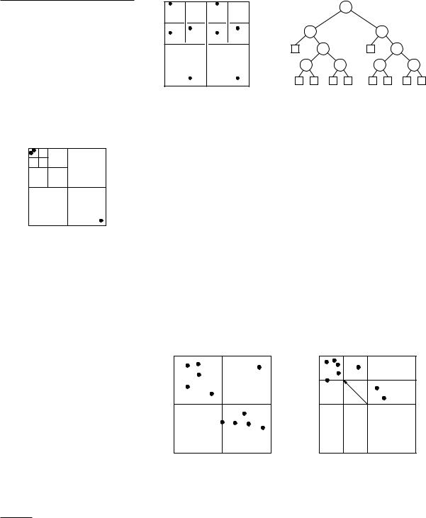
gives us a BSP tree on the set G(S). Figure 12.9 illustrates this. Notice that |
|
|
|
|
||||||
some splitting lines, 2 and 3 for instance, are in fact the same line; what differs |
|
|
|
|
||||||
is which portion of the line is relevant, but this information is not stored with |
|
|
|
|
||||||
the nodes in the BSP tree. By Lemma 12.6, each leaf region in the resulting |
|
|
|
|
||||||
subdivision intersects only a few objects—at most 1 + 4λ , to be precise. The |
|
|
|
|
||||||
second phase of the algorithm then partitions each leaf region further, until all |
|
|
|
|
||||||
objects are separated. How the second phase is done exactly depends on the |
273 |
|||||||||
Chapter 12
BINARY SPACE PARTITIONS
Figure 12.9
A quadtree subdivision and the corresponding BSP tree.
5 |
6 |
8 |
9 |
|
4 |
|
7 |
2 |
|
|
3 |
|
|
1 |
|
1 |
2 |
4 |
5 |
6 |
3 |
7 |
8 |
9 |
type of objects in S. If the objects are line segments, for example, we can apply Algorithm 2DRANDOMBSP given in Section 12.3 to the segment fragments in each leaf region.
Figure 12.10
Examples of a quadtree split and a shrinking step with k = 4
274
The crucial property of the algorithm we just sketched is that for low-density scenes the first phase produces leaf regions that intersect few objects. Unfortunately, there is one problem: the number of leaf regions can be very large. This happens for example when two guards lie very close together near a corner of the initial square U. Therefore we modify the first phase of the algorithm to guarantee it produces a linear number of leaf regions. This is done as follows.
The first modification is that we do not continue subdividing until each region has only one guard in it, but instead we stop when the region contains k or fewer guards, for some suitable parameter k 1. The reason for this and the choice of k will be discussed later.
The second modification is the following. Suppose that in the recursive subdivision procedure we have to subdivide a square σ . Consider the four quadrants of σ . If at least two of them contain more than k guards in their interior, then we proceed as before by applying a quadtree split: we partition σ into its four quadrants by first splitting it with a vertical line v(σ ) and then splitting each half with a horizontal line h(v)—see Figure 12.10. After applying the quadtree split, we recurse on the quadrants. If none of the quadrants
quadtree split |
|
shrinking step |
σ
h(σ )
h(σ )
v(σ ) |
v(σ ) |
contains more than k guards, we also perform a quadtree split; in this case the four quadrants all become leaf regions. If there is exactly one quadrant, say σ , with more than k guards in it we have to be careful: all guards could be very close to a corner, and then it may take many quadtree splits before we finally separate them—see also Lemma 14.1. Therefore we perform a shrinking step. Intuitively, we shrink σ until at least k guards are not in the interior of σ . More

precisely, a shrinking step proceeds as follows. Assume that σ is the north-west quadrant of σ ; the other three cases are handled in a symmetrical fashion. We shrink σ by moving its bottom-right corner diagonally to the north-west—σ thus remains a square during the shrinking process—until at least k guards are outside the interior of σ . With a slight abuse of notation, we use σ to denote the shrunk quadrant. Notice that σ has at least one guard on its boundary. We partition σ by first splitting it with a vertical line v(σ ) through the right edge of σ , and then splitting the two resulting parts with a horizontal line h(σ ) through the bottom edge of σ —see Figure 12.10. This partitions σ into four regions, two of which are squares. In particular σ , the only region that can contain more than k guards and therefore may have to be split further, is a square.
Algorithm PHASE1 summarizes the recursive splitting procedure.
Algorithm PHASE1(σ , G, k)
Input. A region σ , a set G of guards in the interior of σ , and an integer k 1. Output. A BSP tree T such that each leaf region contains at most k guards.
1.if card(G) k
2.then Create a BSP tree T consisting of a single leaf node.
3.else if exactly one quadrant of σ contains more than k guards in its
interior
4.then Determine the splitting lines v(σ ) and h(σ ) for a shrink-
ing step, as explained above.
5.else Determine the splitting lines v(σ ) and h(σ ) for a quadtree
split, as explained above.
6.Create a BSP tree T with three internal nodes; the root of T storesv(σ ) as its splitting line, and both children of the root store h(σ ) as their splitting line.
7.Replace each leaf µ of T by a BSP tree Tµ computed recursively on the region corresponding to µ and the guards inside that region.
8.return T
Lemma 12.7 PHASE1(U, G(S), k) produces a BSP tree with O(n/k) leaves, where each leaf region intersects at most k + 4λ objects.
Proof. We first prove the bound on the number of leaves. This number is one more than the number of internal nodes, and so it suffices to bound the latter number.
Let N(m) denote the maximum number of internal nodes in a BSP tree created by PHASE1(σ , G, k) when card(G) = m. If m k, no splits are performed, and so N(m) = 0 in this case. Otherwise, a quadtree split or a shrinking step is applied to σ . This results in three internal nodes, and four regions in which we recurse. Let m1, . . . , m4 denote the numbers of guards in the four regions, and let I := {i : 1 i 4 and mi > k}. Since a region that contains k or fewer guards is a leaf region, we know that N(mi) = 0 for i I. Hence,
N(m) |
0 |
if m k |
3 + ∑i I N(mi) |
otherwise |
We will prove by induction that N(m) max(0, (6m/k) −3). This is obviously true for m k, and so we now assume that m > k. A guard can be in the interior
Section 12.5
BSP TREES FOR LOW-DENSITY
SCENES
275
Chapter 12
BINARY SPACE PARTITIONS
σ |
σ |
276
of at most one region, which means that ∑i I mi m. If at least two quadrants of σ contain more than k guards, then card(I) 2 and we have
N(m) 3 + ∑N(mi) 3 + |
∑(6mi/k) −card(I) ·3 6m/k −3, |
i I |
i I |
as claimed. If none of the quadrants contains more than k guards, then the four regions are all leaf regions and N(m) = 3. Together with the assumption m > k, this implies N(m) (6m/k) −3. The remaining case is where exactly one quadrant contains more than k guards. In this case we do a shrinking step. Because of the way a shrinking step is performed, a shrunk quadrant contains fewer than m −k guards and the other resulting regions contain at most k guards. Hence, in this case we have
N(m) 3 + N(m −k) 3 + (6(m −k)/k −3) 6m/k −3.
So in all cases N(m) (6m/k) −3, as claimed. This proves the bound on the number of internal nodes.
It remains to prove that each leaf region intersects at most k + 4λ objects. By construction, a leaf region contains at most k guards in its interior. Hence, if a leaf region is a square, Lemma 12.6 implies that it intersects k + 4λ objects. There can also be leaf regions, however, that are not square, and then we cannot apply Lemma 12.6 directly. A non-square leaf region σ must have been produced in a shrinking step, as shown in Figure 12.10. Recall that the shrinking process stops as soon as k or more guards are not in the interior of the shrunk quadrant σ . At least one of these guards must be on the boundary of σ , and in fact the number of guards exterior to σ (not counting the guards on the boundary of σ ) must be less than k. This implies that σ can be covered by a square with at most k guards in its interior; this square is shown in gray in the figure in the margin. By Lemma 12.6, this square intersects at most k + 4λ objects, and so σ intersects at most that many objects as well. 

Lemma 12.7 explains why it can be advantageous to use a value for k that is larger than 1: the larger k is, the fewer leaf regions we will have. On the other hand, a larger k will also mean more objects per leaf region. A good choice of k is therefore one that reduces the number of leaf regions as much as possible, without significantly increasing the number of objects per leaf region. Setting k := λ will do this: the number of leaf regions will decrease by a factor λ (as compared with k = 1), while the maximum number of objects per leaf region does not increase asymptotically—it only goes from 1 + 4λ to 5λ .
There is one problem, however: we do not know λ , the density of the input scene, and so we cannot use it as a parameter in the algorithm. Therefore we use the following trick. We guess a small value for λ , say λ = 2. Then we run PHASE1 with our guess as the value of k, and we check whether each leaf region in the resulting BSP tree intersects at most 5k objects. If so, we proceed with the second phase of the algorithm; otherwise, we double our guess and try again. This leads to the following algorithm.

Algorithm LOWDENSITYBSP2D(S)
Input. A set S of n objects in the plane.
Output. A BSP tree T for S.
1.Let G(S) be the set of 4n bounding-box vertices of the objects in S.
2.k ← 1; done ← false; U ← a bounding square of S
3.while not done
4.do k ← 2k; T ←PHASE1(U, G(S), k); done ← true
5.for each leaf µ of T
6.do Compute the set S(µ ) of object fragments in the region of µ .
7. |
if card(S(µ )) > 5k then done ← false |
8.for each leaf µ of T
9.do Compute a BSP tree Tµ for S(µ ) and replace µ by Tµ .
10.return T
When the input S consists of non-intersecting segments in the plane, we can use 2DRANDOMBSP to compute the BSPs in line 9, leading to the following result.
Theorem 12.8 For any set S of n disjoint line segments in the plane, there is a BSP of size O(n log λ ), where λ is the density of S.
Proof. By Lemma 12.7, PHASE1(U, G(S), k) results in a BSP tree where each leaf region intersects at most k + 4λ objects. Hence, the test in line 7 of LOWDENSITYBSP2D is guaranteed to be false if k λ . (If k < λ , the test may or may not be false.) The while-loop therefore ends, at the latest, when k becomes larger than λ for the first time. Since k doubles every time, this implies k 2λ when we get to the second phase in line 8.
Let k denote the value of k when we get to line 8. We have just argued that k 2λ . The test in line 7 guarantees that each leaf region intersects at most 5k segments. Hence, according to Lemma 12.1, each tree Tµ has (expected) size O(k log k ) when 2DRANDOMBSP is used in line 9. Because there are O(n/k ) leaf regions, the total size of the BSP tree is O(n log k ). Since k 2λ , this proves the theorem. 

The bound in Theorem 12.8 is never worse than O(n log n). In other words, the algorithm described above is as good as the algorithm given in Section 12.3 in the worst case, but it provably profits when the density of the input is low.
Recall that the reason for introducing the concept of density was the quadratic worst-case bound for BSPs for triangles in R3. The algorithm that we have just described works very well for segments in the plane: it produces a BSP whose size is O(n log n) in the worst case and O(n) when the density of the input is a constant. What happens when we apply this approach to a set of triangles in R3? As it turns out, it also leads to good results in this case, as stated in the next theorem. (Exercise 12.18 asks you to prove this theorem.)
Theorem 12.9 For any set S of n disjoint triangles in R3, there is a BSP of size O(nλ ), where λ is the density of S.
Section 12.5
BSP TREES FOR LOW-DENSITY
SCENES
277

Chapter 12
BINARY SPACE PARTITIONS
The bound in Theorem 12.9 interpolates nicely between O(n) and O(n2) as λ varies from 1 to n. Therefore the algorithm produces a BSP whose size is optimal in the worst case. But the result is even stronger: the O(nλ ) bound is optimal for all values of λ : for any n and any λ with 1 λ n there is a collection of n triangles in R3 whose density is λ and for which any BSP must have size Ω(nλ ).
12.6 Notes and Comments
BSP trees are popular in many application areas, in particular in computer graphics. The application mentioned in this chapter is to performing hiddensurface removal with the painter’s algorithm [185]. Other applications include shadow generation [124], set operations on polyhedra [292, 370], and visibility preprocessing for interactive walkthroughs [369]. BSP trees have also been used in cell decomposition methods in motion planning [36], for range searching [60], and as general indexing structure in GIS [294]. Two other well-known structures, kd-trees and quadtrees, are in fact special cases of BSP trees, where only orthogonal splitting planes are used. Kd-trees were discussed extensively in Chapter 5 and quadtrees will be discussed in Chapter 14.
The study of BSP trees from a theoretical point of view was initiated by Paterson and Yao [317]; the results in Sections 12.3 and 12.4 come from their paper. They also proved bounds on BSPs in higher dimensions: any set of (d −1)-dimensional simplices in Rd , with d 3, admits a BSP of size O(nd−1). Paterson and Yao also obtained results for orthogonal objects in higher dimensions [318]. For instance, they proved that any set of orthogonal rectangles in R3 admits a BSP of size O(n√n), and that this bound is tight in the worst case. Below we discuss several of the results that have been obtained since. A more extensive overview has been given by Toth´ [373].
For a long time it was unknown whether any set of n disjoint line segments in the plane would admit a BSP of size O(n), but Toth´ [372] proved that this is not the case, by constructing a set of segments for which any BSP must have size Ω(n log n/ log log n). Note that there is still a small gap between this lower bound and the currently known upper bound, which is O(n log n). There are several special cases, however, where an O(n) size BSP is possible. For example, Paterson and Yao [317] have shown that any set of n disjoint segments
|
in the plane that are all either horizontal or vertical admit a BSP of size O(n). |
|
The same result was achieved by d’Amore and Franciosa [138]. Toth´ [371] |
|
generalized this result to segments with a limited number of orientations. Other |
|
special cases where a linear-size BSP is always possible are for line segments |
|
with more or less the same length [54] and, as we have already seen in this |
|
chapter, for sets of objects of constant density. |
|
In Section 12.5, we studied BSPs for low-density scenes. This was inspired by |
|
the observation that the worst-case size of BSPs for 3-dimensional scenes has |
278 |
little to do with their practical performance. A similar situation arises frequently |

in the study of geometric algorithms: often one can come up with input sets for which the algorithm at hand is not very efficient, but in many cases such input sets are not very realistic. This can have two disadvantages. First, a worstcase analysis of the algorithm may not be very informative as to whether the algorithm is useful in practice. Second, since algorithms are typically designed to have the best worst-case performance, they may be geared towards handling situations that will not arise in practice and therefore they may be needlessly complicated. The underlying reason for this is that, usually, the running time of a geometric algorithm not only is determined by the size of the input but also is strongly influenced by the shape of the input objects and their spatial distribution. To overcome this problem, one can try to define a parameter that captures the geometry of the input—just as we did in Section 12.5.
The parameter that has been used most often in this context is fatness. A triangle is called β -fat if all its angles are at least β . It has been shown that the complexity of the union of n intersecting β -fat triangles in the plane is near-linear in n if β is a constant [268]; currently, the best known bound is O((1/β ) log(1/β ) · n log log n) [314]. The concept of fatness has been generalized to arbitrary convex objects, and even to non-convex objects. One of the most general definitions was given by van der Stappen [362], who defined an object o in Rd to be β -fat if the following holds: for any ball B whose center lies in o and that does not fully contain o in its interior, we have that vol(o ∩ B) β · vol(B), where vol(·) denotes the volume. There are many problems that can be solved more efficiently for fat objects than for general objects. Examples are range searching and point location [51, 60], motion planning [363], hidden-surface removal [229], ray shooting [21, 49, 53, 228], and computing depth orders [53, 228].
The parameter used in Section 12.5, density, has also been studied a lot. It can be shown that any set of disjoint β -fat objects has density O(1/β ) [55, 362], and so any result obtained for low-density scenes immediately gives a result for disjoint fat objects. The algorithm for constructing a BSP for low-density scenes described in Section 12.5 is a modified and slightly improved version of the construction by de Berg [51]. Some of the results mentioned above for fat objects are in fact based on this construction [60, 363] and hence also apply to low-density scenes.
Section 12.7
EXERCISES
12.7Exercises
12.1Prove that PAINTERSALGORITHM is correct. That is, prove that if (some part of) an object A is scan-converted before (some part of) object B is scan-converted, then A cannot lie in front of B.
12.2Let S be a set of m polygons in the plane with n vertices in total. Let T be a BSP tree for S of size k. Prove that the total complexity of the
fragments generated by the BSP is O(n + k). |
279 |

Chapter 12
BINARY SPACE PARTITIONS
280
12.3Give an example of a set of line segments in the plane where the greedy method of constructing an auto-partition (where the splitting line (s) is taken that induces the least number of cuts) results in a BSP of quadratic size.
12.4Give an example of a set S of n non-intersecting line segments in the plane for which a BSP tree of size n exists, whereas any auto-partition of S has size at least 4n/3 .
12.5Give an example of a set S of n disjoint line segments in the plane such that any auto-partition for S has depth Ω(n).
12.6We have shown that the expected size of the partitioning produced by 2DRANDOMBSP is O(n log n). What is the worst-case size?
12.7Suppose we apply 2DRANDOMBSP to a set of intersecting line segments in the plane. Can you say anything about the expected size of the resulting BSP tree?
12.8In 3DRANDOMBSP2, it is not described how to find the cells that must be split when a splitting plane is added, nor is it described how to perform the split efficiently. Work out the details for this step, and analyze the running time of your algorithm.
12.9Give a deterministic divide-and-conquer algorithm that constructs a BSP tree of size O(n log n) for a set of n line segments in the plane. Hint: Use as many free splits as possible and use vertical splitting lines otherwise.
12.10Let C be a set of n disjoint unit discs—discs of radius 1—in the plane. Show that there is a BSP of size O(n) for C. Hint: Start by using a suitable collection of vertical lines of the form x = 2i for some integer i.
12.11BSP trees can be used for a variety of tasks. Suppose we have a BSP on the edges of a planar subdivision.
a.Give an algorithm that uses the BSP tree to perform point location on the subdivision. What is the worst-case query time?
b.Give an algorithm that uses the BSP tree to report all the faces of the subdivision intersected by a query segment. What is the worst-case query time?
c.Give an algorithm that uses the BSP tree to report all the faces of the subdivision intersected by an axis-parallel query rectangle. What is the worst-case query time?
12.12In Chapter 5 kd-trees were introduced. Kd-trees can also store segments instead of points, in which case they are in fact a special type of BSP tree, where the splitting lines for nodes at even depth in the tree are horizontal and the splitting lines at odd levels are vertical.
a.Discuss the advantages and/or disadvantages of BSP trees over kdtrees.

b.For any set of two non-intersecting line segments in the plane there exists a BSP tree of size 2. Prove that there is no constant c such that for any set of two non-intersecting line segments there exists a kd-tree of size at most c.
12.13Prove that the density of any set of disjoint discs in the plane is at most 9. (Thus the dependency is independent of the number of discs.) Use this
to show that any set of n disjoint discs in the plane has a BSP of size O(n). Generalize the result to higher dimensions.
12.14A triangle is called α -fat if all its angles are at least α . Prove that any set of α -fat disjoint triangles in the plane has density O(1/α ). Use this to show that any set of n disjoint α -fat triangles admits a BSP of size O(n log(1/α )), and argue that this implies that any set of n disjoint squares admits a BSP of size O(n).
12.15Give an example of a set of n triangles whose density is a constant
such that any auto-partition—that is, any BSP that only uses splitting planes containing input triangles—has size Ω(n2). (This example shows
that the randomized algorithm of Section 12.4 can produce a BSP of expected size Ω(n2) even when the density of the input set of triangles is a constant.) Hint:Use a set of triangles that are all parallel to the z-axis and whose projections onto the xy-plane form a grid.
12.16Let T be a set of disjoint triangles in the plane. Instead of taking the bounding-box vertices of the triangles as guards, we could also take the vertices of the triangles themselves. Show that this is not a good set of guards by giving a counterexample to Lemma 12.6 if the guards are defined in this way. Can you give a counterexample for the case where all triangles are equilateral triangles?
12.17Show that Algorithm LOWDENSITYBSP2D can be implemented so that it runs in O(n2) time.
12.18Generalize Algorithm LOWDENSITYBSP2D to R3, and analyze the size of the resulting BSP.
Section 12.7
EXERCISES
281