9Delaunay Triangulations
Height Interpolation
When we talked about maps of a piece of the earth’s surface in previous chapters, we implicitly assumed there is no relief. This may be reasonable for a country like the Netherlands, but it is a bad assumption for Switzerland. In this chapter we set out to remedy this situation.
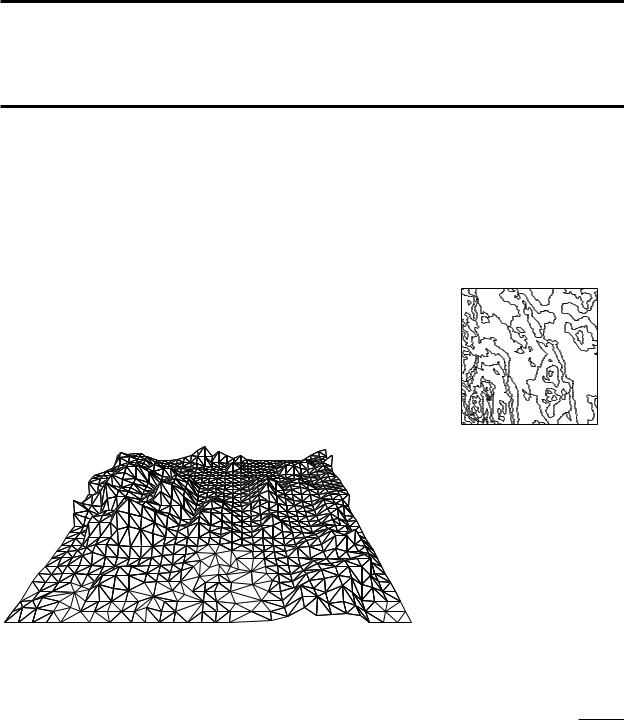
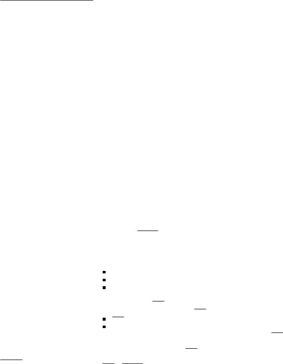
We can model a piece of the earth’s surface as a terrain. A terrain is a 2-dimensional surface in 3-dimensional space with a special property: every vertical line intersects it in a point, if it intersects it at all. In other words, it is the graph of a function f : A R2 → R that assigns a height f (p) to every point p in the domain, A, of the terrain. (The earth is round, so on a global scale terrains defined in this manner are not a good model of the earth. But on a more local scale terrains provide a fairly good model.) A terrain can be visualized with a perspective drawing like the one in Figure 9.1, or with contour lines—lines of equal height—like on a topographic map.
|
Figure 9.1 |
|
A perspective view of a terrain |
Of course, we don’t know the height of every point on earth; we only know it |
|
where we’ve measured it. This means that when we talk about some terrain, we |
|
only know the value of the function f at a finite set P A of sample points. From |
|
the height of the sample points we somehow have to approximate the height |
|
at the other points in the domain. A naive approach assigns to every p A the |
|
height of the nearest sample point. However, this gives a discrete terrain, which |
191 |
Chapter 9
DELAUNAY TRIANGULATIONS
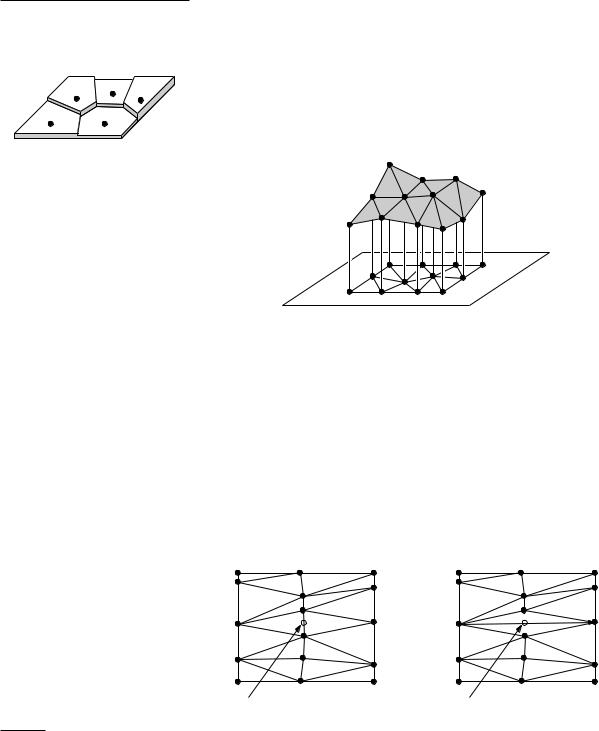
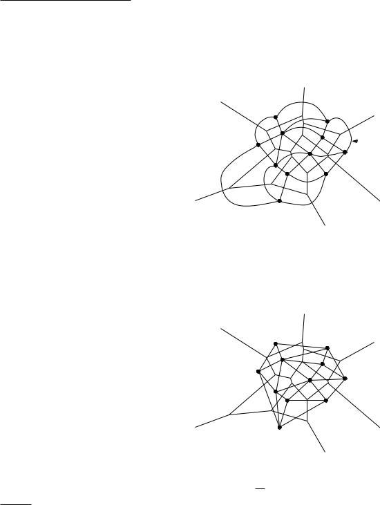
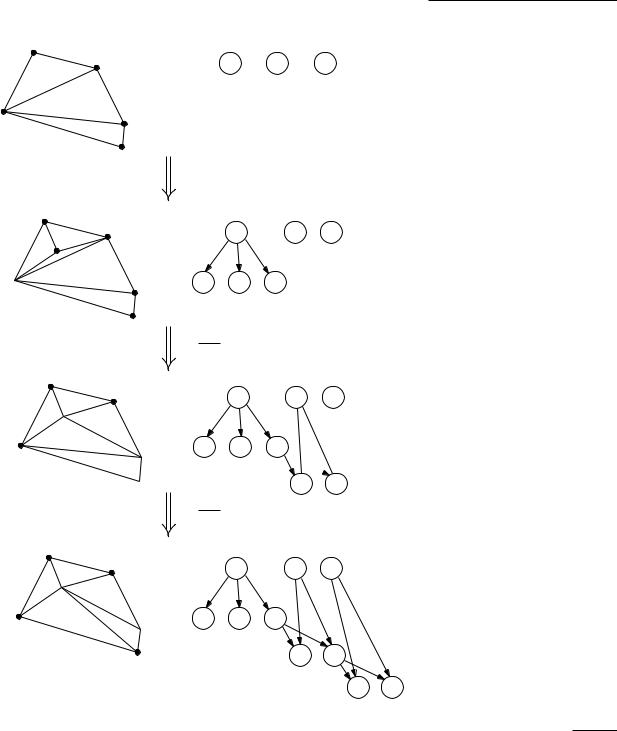
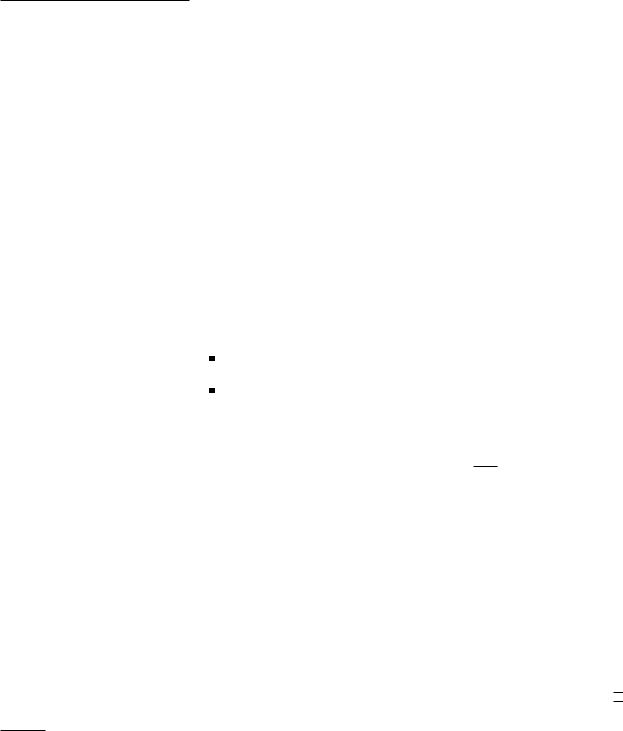
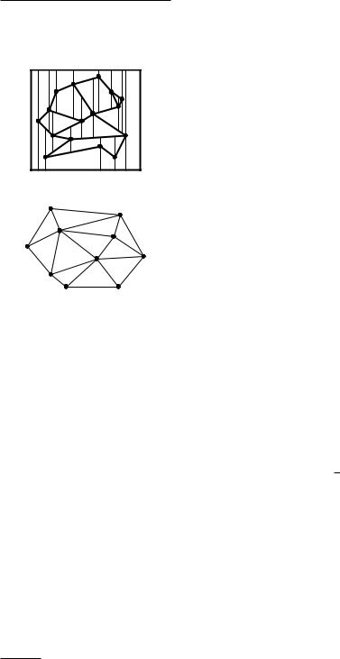
Figure 9.2
Obtaining a polyhedral terrain from a set of sample points
doesn’t look very natural. Therefore our approach for approximating a terrain is as follows. We first determine a triangulation of P: a planar subdivision whose bounded faces are triangles and whose vertices are the points of P. (We assume that the sample points are such that we can make the triangles cover the domain of the terrain.) We then lift each sample point to its correct height, thereby mapping every triangle in the triangulation to a triangle in 3-space. Figure 9.2 illustrates this. What we get is a polyhedral terrain, the graph of a continuous function that is piecewise linear. We can use the polyhedral terrain as an approximation of the original terrain.
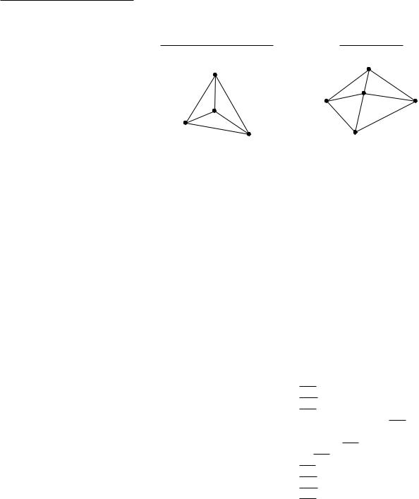
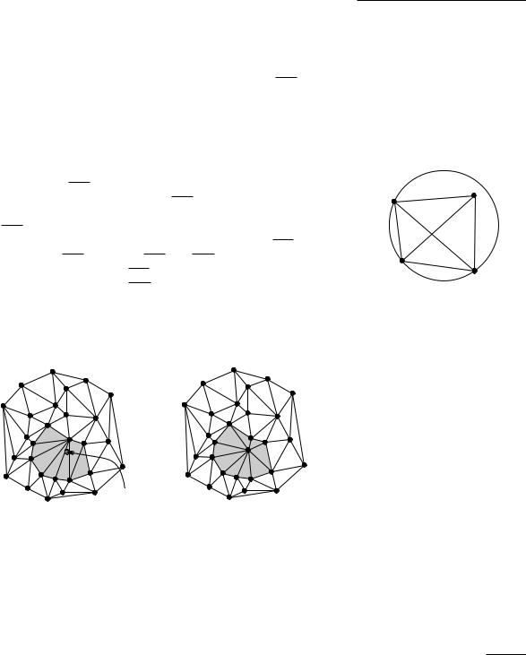
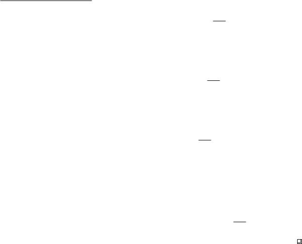
The question remains: how do we triangulate the set of sample points? In general, this can be done in many different ways. But which triangulation is the most appropriate one for our purpose, namely to approximate a terrain? There is no definitive answer to this question. We do not know the original terrain, we only know its height at the sample points. Since we have no other information, and the height at the sample points is the correct height for any triangulation, all triangulations of P seem equally good. Nevertheless, some triangulations look more natural than others. For example, have a look at Figure 9.3, which shows two triangulations of the same point set. From the heights of the sample points we get the impression that the sample points were taken from a mountain ridge. Triangulation (a) reflects this intuition. Triangulation (b), however, where one single edge has been “flipped,” has introduced a narrow valley cutting through the mountain ridge. Intuitively, this looks wrong. Can we turn this intuition into a criterion that tells us that triangulation (a) is better than triangulation (b)?
0 |
1240 |
|
|
0 |
1000 |
|
|
|
980 |
10 |
q |
|
|
|
990 |
6 |
1008 |
|
Figure 9.3 |
4 |
890 |
|
Flipping one edge can make a big |
height = 985 |
||
(a) |
|||
difference |
|
19 |
0 |
20 |
0 |
|
|
36 |
10 |
28 |
6 |
|
|
23 |
4 |
height = 23
1240 |
19 |
|
|
|
|
|
1000 |
20 |
q |
980 |
|
|
36 |
|
|
|
|
|
990 |
|
|
1008 |
28 |
890 |
23 |
|
|
||
(b)
192 |
The problem with triangulation (b) is that the height of the point q is deter- |
mined by two points that are relatively far away. This happens because q lies in the middle of an edge of two long and sharp triangles. The skinniness of these triangles causes the trouble. So it seems that a triangulation that contains small angles is bad. Therefore we will rank triangulations by comparing their smallest angle. If the minimum angles of two triangulations are identical, then we can look at the second smallest angle, and so on. Since there is only a finite number of different triangulations of a given point set P, this implies that there must be an optimal triangulation, one that maximizes the minimum angle. This will be the triangulation we are looking for.
Section 9.1
TRIANGULATIONS OF PLANAR POINT
SETS
9.1 Triangulations of Planar Point Sets
Let P := {p1, p2, . . . , pn} be a set of points in the plane. To be able to formally |
|
|
define a triangulation of P, we first define a maximal planar subdivision as |
|
|
a subdivision S such that no edge connecting two vertices can be added to |
|
|
S without destroying its planarity. In other words, any edge that is not in S |
|
|
intersects one of the existing edges. A triangulation of P is now defined as a |
|
|
maximal planar subdivision whose vertex set is P. |
|
|
With this definition it is obvious that a triangulation exists. But does it |
|
|
consist of triangles? Yes, every face except the unbounded one must be a |
|
|
triangle: a bounded face is a polygon, and we have seen in Chapter 3 that any |
|
|
polygon can be triangulated. What about the unbounded face? It is not difficult |
|
|
to see that any segment connecting two consecutive points on the boundary of |
|
|
the convex hull of P is an edge in any triangulation T. This implies that the |
|
|
union of the bounded faces of T is always the convex hull of P, and that the |
|
|
unbounded face is always the complement of the convex hull. (In our application |
|
|
this means that if the domain is a rectangular area, say, we have to make sure |
|
|
that the corners of the domain are included in the set of sample points, so that |
|
|
the triangles in the triangulation cover the domain of the terrain.) The number |
|
|
of triangles is the same in any triangulation of P. This also holds for the number |
|
|
of edges. The exact numbers depend on the number of points in P that are on |
|
|
the boundary of the convex hull of P. (Here we also count points in the interior |
convex hull boundary |
|
of convex hull edges. Hence, the number of points on the convex hull boundary |
|
|
is not necessarily the same as the number of convex hull vertices.) This is made |
|
|
precise in the following theorem. |
|
|
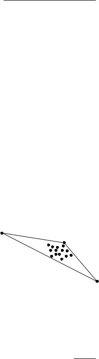
Theorem 9.1 Let P be a set of n points in the plane, not all collinear, and let k |
|
|
denote the number of points in P that lie on the boundary of the convex hull |
|
|
of P. Then any triangulation of P has 2n −2 −k triangles and 3n −3 −k edges. |
|
|
Proof. Let T be a triangulation of P, and let m denote the number of triangles |
|
|
of T. Note that the number of faces of the triangulation, which we denote by |
|
|
n f , is m + 1. Every triangle has three edges, and the unbounded face has k |
|
|
edges. Furthermore, every edge is incident to exactly two faces. Hence, the |
|
|
total number of edges of T is ne := (3m + k)/2. Euler’s formula tells us that |
|
|
n −ne + n f = 2. |
193 |
|
Chapter 9
DELAUNAY TRIANGULATIONS
Plugging the values for ne and n f into the formula, we get m = 2n −2 −k, which in turn implies ne = 3n −3 −k. 

Let T be a triangulation of P, and suppose it has m triangles. Consider the 3m angles of the triangles of T, sorted by increasing value. Let α1, α2, . . . , α3m be the resulting sequence of angles; hence, αi α j, for i < j. We call A(T) := (α1, α2, . . . , α3m) the angle-vector of T. Let T be another triangulation of the
same point set P, and let A(T ) := (α1, α2, . . . , α3m) be its angle-vector. We say that the angle-vector of T is larger than the angle-vector of T if A(T) is
lexicographically larger than A(T ), or, in other words, if there exists an index i with 1 i 3m such that
α j = α j for all j < i, and αi > αi .
We denote this as A(T) > A(T ). A triangulation T is called angle-optimal if A(T) A(T ) for all triangulations T of P. Angle-optimal triangulations are interesting because, as we have seen in the introduction to this chapter, they are good triangulations if we want to construct a polyhedral terrain from a set of sample points.
s |
q
|
p |
r |
|
|
|
|
|
b |
|
a |
C |
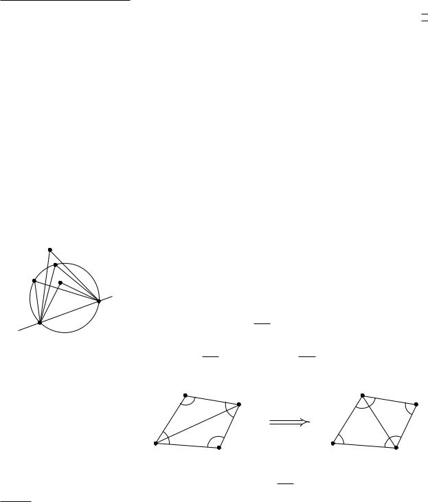
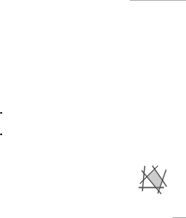
Figure 9.4
Flipping an edge
194
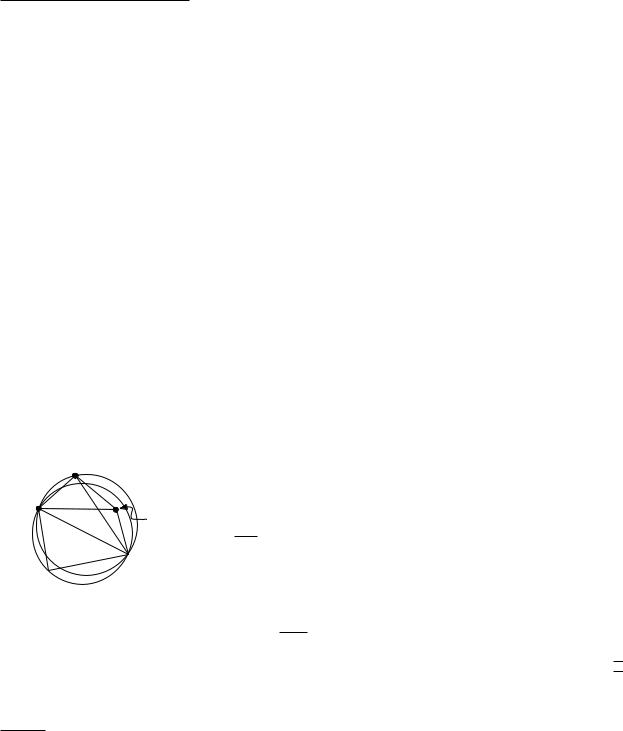
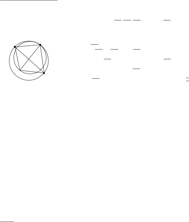
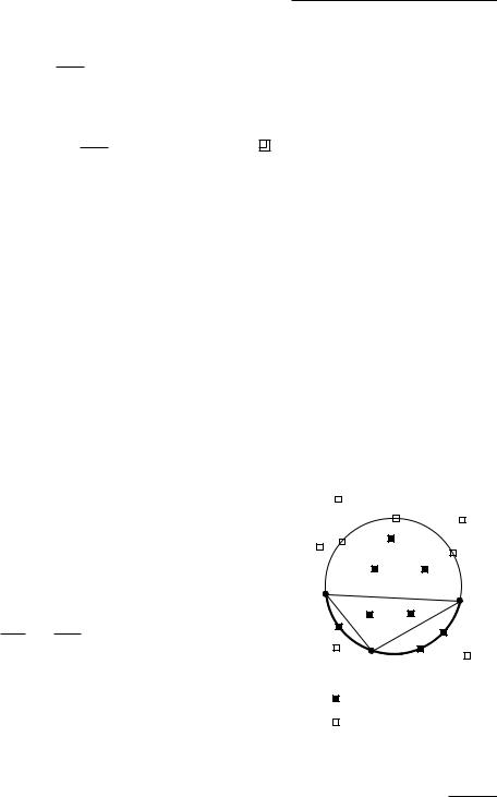
Below we will study when a triangulation is angle-optimal. To do this it is useful to know the following theorem, often called Thales’s Theorem. Denote the smaller angle defined by three points p, q, r by pqr.
Theorem 9.2 Let C be a circle, a line intersecting C in points a and b, and p, q, r, and s points lying on the same side of . Suppose that p and q lie on C, that r lies inside C, and that s lies outside C. Then
arb > apb = aqb > asb.
Now consider an edge e = pi p j of a triangulation T of P. If e is not an edge of the unbounded face, it is incident to two triangles pi p j pk and pi p j pl . If these two triangles form a convex quadrilateral, we can obtain a new triangulation T by removing pi p j from T and inserting pk pl instead. We call this operation an edge flip. The only difference in the angle-vector of T and T are the six
pl pl
α2 |
α3 |
p j |
|
α |
α5 |
edge flip |
α |
4 |
|
|
|
2 |
|
|
α1 |
α6 |
|
α |
α |
|
α |
|
|||
pi |
4 |
pi |
1 |
||
|
|
3 |
|||
|
|
|
pk |
|
|
p j
α6
α5
pk |
angles α1, . . . , α6 in A(T), which are replaced by α1, . . . , α6 in A(T ). Figure 9.4 illustrates this. We call the edge e = pi p j an illegal edge if
min αi < min αi .
1 i 6 1 i 6
 p
p 
 G
G Vor(
Vor(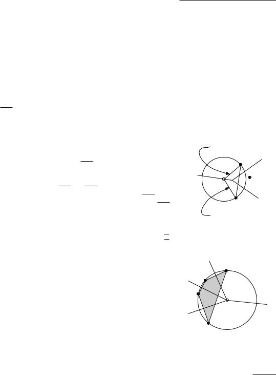


 p
p 


 ∆
∆

 ∆
∆ ∆
∆


 q
q