

1greenacre_m_primicerio_r_multivariate_analysis_of_ecological
.pdfMULTIVARIATE ANALYSIS OF ECOLOGICAL DATA
60

CHAPTER 5
Measures of Distance between Samples:
Non-Euclidean
Euclidean distances are special because they conform to our physical concept of distance. But there are many other distance measures which can be defined between multivariate samples. These non-Euclidean distances are of different types: some still satisfy the basic axioms of what mathematicians call a distance metric, while others are not even true metrics but still make good sense as a measure of difference between samples in the context of certain data. In this chapter we shall consider several non-Euclidean distance measures that are popular in the environmental sciences: the Bray-Curtis dissimilarity, the L1 distance (also called the city-block or Manhattan distance) and the Jaccard index for presence-absence data. We also consider how to measure dissimilarity between samples for which we have mixed-scale data.
Contents |
|
The axioms of distance . . . . . . . . . . . . . . . . . . . . . . . . . . . . . . . . . . . . . . . . . . . . . . . . . . . . . . . . . . . . |
61 |
Bray-Curtis dissimilarity . . . . . . . . . . . . . . . . . . . . . . . . . . . . . . . . . . . . . . . . . . . . . . . . . . . . . . . . . . . |
62 |
Bray-Curtis dissimilarity versus chi-square . . . . . . . . . . . . . . . . . . . . . . . . . . . . . . . . . . . . . . . . . . . . |
64 |
L1 distance (city-block) . . . . . . . . . . . . . . . . . . . . . . . . . . . . . . . . . . . . . . . . . . . . . . . . . . . . . . . . . . . |
67 |
Dissimilarity measures for presence−absence data . . . . . . . . . . . . . . . . . . . . . . . . . . . . . . . . . . . . . |
68 |
Distances for mixed-scale data . . . . . . . . . . . . . . . . . . . . . . . . . . . . . . . . . . . . . . . . . . . . . . . . . . . . . |
70 |
SUMMARY: Measures of distance between samples: non-Euclidean . . . . . . . . . . . . . . . . . . . . . . . . . |
73 |
In mathematics, a true measure of distance, also called a metric, obeys three prop- The axioms of distance |
|
erties. These metric axioms are as follows (Exhibit 5.1), where dab denotes the |
|
distance between objects a and b: |
|
1.dab dba
2. dab 0 |
and 0 |
if and only if a b |
(5.1) |
3.dab dac dca
61

|
|
MULTIVARIATE ANALYSIS OF ECOLOGICAL DATA |
Exhibit 5.1: |
c |
|
Illustration of the triangle |
|
|
inequality for distances in |
b |
b |
Euclidean space |
|
|
|
|
c |
a |
dab < dac + dcb |
a |
dab = dac + dcb |
The first two axioms seem self-evident: the first says that the distance from a to b is the same as from b to a, in other words the measure is symmetric; the second says that distances are always positive except when the objects are identical, in which case the distance is necessarily 0. The third axiom, called the triangle inequality, may also seem intuitively obvious but is the more difficult one to satisfy. If we draw a triangle abc in our Euclidean world, for example in Exhibit 5.1, then it is obvious that the distance from a to b must be shorter than the sum of the distances via another point c, that is from a to c and from c to b. The triangle inequality can only be an equality if c lies exactly on the line connecting a and b (see the right hand sketch in Exhibit 5.1).
But there are many apparently acceptable measures of distance that do not satisfy this property: with those it would be theoretically possible to get a “route” from a to b via a third point c which is shorter than from a to b “directly”. Because such measures that do not satisfy the triangle inequality are not true distances (in the mathematical sense) they are usually called dissimilarities.
Bray-Curtis dissimilarity When it comes to species abundance data collected at different sampling locations, the Bray-Curtis (or S¿rensen) dissimilarity is one of the most well-known ways of quantifying the difference between samples. This measure appears to be a very reasonable way of achieving this goal but it does not satisfy the triangle inequality axiom, and hence is not a true distance (we shall discuss the implications of this in later chapters when we analyse Bray-Curtis dissimilarities). To illustrate its definition, we consider again the count data for the last two samples of Exhibit 1.1, which we recall here:
|
a |
b |
c |
d |
e |
Sum |
|
|
|
|
|
|
|
s29 |
11 |
0 |
7 |
8 |
0 |
26 |
s30 |
24 |
37 |
5 |
18 |
1 |
85 |
|
|
|
|
|
|
|
62

MEASURES OF DISTANCE BETWEEN SAMPLES: NON-EUCLIDEAN
One of the assumptions of the Bray-Curtis measure is that the sampled areas or volumes are of the same size. This is because dissimilarity will be computed on raw counts, not on relative counts, so the fact that there is higher overall abundance at site s30 is part of the difference between these two samples – that is, “size” and “shape” of the count vectors will be taken into account in the measure.1
The computation involves summing the absolute differences between the counts and dividing this by the sum of the abundances in the two samples, denoted here by b:
bs29, s30 |
= |
|
|
11 − 24 |
|
+ |
|
0 − 37 |
|
+ |
|
7 − 5 |
|
+ |
|
8 − 18 |
|
+ |
|
0 − 1 |
|
|
= |
63 |
= 0.568 |
|
|
|
|
|
|
|
|
|
|
||||||||||||||||
|
|
|
|
|
|
|
|
|
|
|
|
|
|
|
|
|
|
|
|
|
|
||||
|
26 + 85 |
111 |
|
||||||||||||||||||||||
The general formula for calculating the Bray-Curtis dissimilarity between samples i and i is as follows, supposing that the counts are denoted by nij and that their sample (row) totals are ni :
|
|
J |
|
|
|
|
||
|
= |
∑ |
|
nij |
−ni ′j |
|
|
|
|
|
|
||||||
b |
j = 1 |
|
|
|
|
|
(5.2) |
|
ii ′ |
|
ni + +ni ′+ |
||||||
|
|
|||||||
This measure takes on values between 0 (for identical samples: nij ni j for all j) and 1 (samples completely disjoint; that is, when there is a nonzero abundance of a species in one sample, then it is zero in the other: nij > 0 implies ni j 0) – hence it is often multiplied by 100 and interpreted as a percentage. Exhibit 5.2 shows part of the Bray-Curtis dissimilarities between the 30 samples (the caption points out a violation of the triangle inequality).
If the Bray-Curtis dissimilarity is subtracted from 100, a measure of similarity is obtained, called the Bray-Curtis index. For example, the similarity between sites s25 and s4 is 100 93.9 6.1%, which is the lowest amongst the values displayed in Exhibit 5.2; whereas the highest similarity is for sites s25 and s26: 100 13.7 86.3%. Checking back to the data in Exhibit 1.1 one can verify the similarity between sites s25 and s26, compared to the lack of similarity between s25 and s4.
1 In fact, the Bray-Curtis dissimilarity can be computed on relative abundances, as we did for the chi-square distance, to take into account only “shape” differences – this point is discussed later. This version is often referred to as the relative Sørensen dissimilarity.
63

MULTIVARIATE ANALYSIS OF ECOLOGICAL DATA
Exhibit 5.2: |
|
s1 |
s2 |
s3 |
s4 |
s5 |
s6 |
· · · |
s24 |
s25 |
s26 |
s27 |
s28 |
s29 |
||
Bray-Curtis dissimilarities, |
|
|||||||||||||||
|
|
|
|
|
|
|
|
|
|
|
|
|
|
|
|
|
multiplied by 100, between |
s2 |
45.7 |
|
|
|
|
|
|
|
|
|
|
|
|
|
|
the 30 samples of Exhibit |
s3 |
|
|
|
|
|
|
|
|
|
|
|
|
|
|
|
29.6 |
48.1 |
|
|
|
|
|
|
|
|
|
|
|
|
|
||
1.1, based on the count |
|
|
|
|
|
|
|
|
|
|
|
|
|
|||
|
|
|
|
|
|
|
|
|
|
|
|
|
|
|
|
|
data for species a to e. |
s4 |
46.7 |
55.6 |
46.7 |
|
|
|
|
|
|
|
|
|
|
|
|
Violations of the triangle |
s5 |
|
|
|
|
|
|
|
|
|
|
|
|
|
|
|
47.7 |
34.8 |
50.8 |
78.6 |
|
|
|
|
|
|
|
|
|
|
|
||
inequality can be easily |
|
|
|
|
|
|
|
|
|
|
|
|||||
|
|
|
|
|
|
|
|
|
|
|
|
|
|
|
|
|
picked out: for example, |
s6 |
52.2 |
22.9 |
52.2 |
69.2 |
41.9 |
|
|
|
|
|
|
|
|
|
|
from s25 to s4 the Bray- |
s7 |
|
|
|
|
|
|
|
|
|
|
|
|
|
|
|
45.5 |
41.5 |
49.1 |
87.0 |
21.2 |
50.9 |
|
|
|
|
|
|
|
|
|
||
Curtis is 93.9, but the sum |
|
|
|
|
|
|
|
|
|
|||||||
· |
· |
· |
· |
· |
· |
· |
|
· |
|
|
|
|
|
|
|
|
|
|
|
|
|
|
|
|
|||||||||
of the values “via s6” from |
|
· |
|
|
|
|
|
|
||||||||
· |
· |
· |
· |
· |
· |
· |
|
· |
|
|
|
|
|
|
||
s25 to s6 and from s6 to |
· |
· |
· |
· |
· |
· |
· |
|
· |
· · |
|
|
|
|
|
|
s4 is 18.6 69.2 87.8, |
s25 |
70.4 |
39.3 |
66.7 |
93.9 |
52.9 |
18.6 |
|
· · · |
46.4 |
|
|
|
|
|
|
which is shorter |
s26 |
|
|
|
|
|
|
|
|
|
|
|
|
|
|
|
69.6 |
32.8 |
60.9 |
92.8 |
41.7 |
15.2 |
|
· · · |
39.3 |
13.7 |
|
|
|
|
|||
|
|
|
|
|
|
|||||||||||
|
s27 |
|
|
|
|
|
|
|
|
|
|
|
|
|
|
|
|
63.6 |
38.1 |
63.6 |
93.3 |
38.2 |
21.5 |
|
· · · |
42.6 |
16.3 |
22.6 |
|
|
|
||
|
s28 |
|
|
|
|
|
|
|
|
|
|
|
|
|
|
|
|
32.5 |
21.5 |
50.0 |
57.7 |
31.9 |
29.5 |
|
· · · |
30.9 |
41.8 |
47.5 |
34.4 |
|
|
||
|
s29 |
|
|
|
|
|
|
|
|
|
|
|
|
|
|
|
|
43.4 |
35.0 |
43.4 |
54.5 |
31.2 |
53.6 |
|
· · · |
39.8 |
64.5 |
58.2 |
61.2 |
34.2 |
|
||
|
s30 |
|
|
|
|
|
|
|
|
|
|
|
|
|
|
|
|
60.7 |
36.7 |
58.9 |
84.5 |
48.0 |
21.6 |
|
· · · |
40.8 |
18.1 |
25.3 |
23.6 |
37.7 |
56.8 |
||
|
|
|
|
|
|
|
|
|
|
|
|
|
|
|
|
|
Bray-Curtis dissimilarity versus chi-square distance
An ecologist would like some recommendation about whether to use BrayCurtis or chi-square on a particular data set. It is not possible to make any absolute statement of which is preferable, but we can point out some advantages and disadvantages of each one. The advantage of the chi-square distance is that it is a true metric, while the Bray-Curtis dissimilarity violates the triangle inequality, which can be problematic when we come to analysing them later. The advantage of Bray-Curtis is that the scale is easy to understand: 0 means the samples are exactly the same, while 100 is the maximum difference that can be observed between two samples. The chi-square, on the other hand, has a maximum which depends on the marginal weights of the data set, and it is difficult to assign any substantive meaning to any particular value. If two samples have the same relative abundances, but different totals, then Bray-Curtis is positive, whereas chi-square is zero. As pointed out in a previous footnote in this chapter, Bray-Curtis dissimilarities can be calculated on the relative abundances (although conventionally the calculation is on raw counts), and in addition we could calculate chi-square distances on the raw counts, without “relativizing” them (although conventionally the calculation is on relative counts). This would make the comparison between the two approaches fairer.
So we also calculated Bray-Curtis on the relative counts and chi-square on the raw counts – Exhibit 5.3 shows parts of the four distance matrices, where the values in each triangular matrix have been strung out column-
64

MEASURES OF DISTANCE BETWEEN SAMPLES: NON-EUCLIDEAN
wise (the column “site pair” shows which pair corresponds to the values in the rows).
SITE PAIR |
B-C raw |
chi2 raw |
B-C rel |
chi2 rel |
|
|
|
|
|
(s2,s1) |
45.679 |
7.398 |
48.148 |
1.139 |
(s3,s1) |
29.630 |
3.461 |
29.630 |
0.855 |
(s4,s1) |
46.667 |
4.146 |
50.000 |
1.392 |
(s5,s1) |
47.692 |
5.269 |
50.975 |
1.093 |
(s6,s1) |
52.212 |
10.863 |
53.058 |
1.099 |
(s7,s1) |
45.455 |
4.280 |
46.164 |
1.046 |
(s8,s1) |
93.333 |
5.359 |
92.593 |
2.046 |
(s9,s1) |
33.333 |
5.462 |
40.741 |
0.868 |
(s10,s1) |
40.299 |
6.251 |
36.759 |
0.989 |
(s11,s1) |
35.714 |
4.306 |
36.909 |
1.020 |
(s12,s1) |
37.500 |
5.213 |
39.762 |
0.819 |
(s13,s1) |
57.692 |
5.978 |
59.259 |
1.581 |
(s14,s1) |
63.265 |
5.128 |
59.091 |
1.378 |
(s15,s1) |
20.755 |
1.866 |
20.513 |
0.464 |
(s16,s1) |
85.714 |
13.937 |
80.960 |
1.700 |
(s17,s1) |
100.000 |
5.533 |
100.000 |
2.258 |
(s18,s1) |
56.897 |
11.195 |
36.787 |
0.819 |
(s19,s1) |
16.923 |
1.762 |
11.501 |
0.258 |
(s20,s1) |
33.333 |
3.734 |
31.987 |
0.800 |
· |
· |
· |
· |
· |
· |
· |
· |
· |
· |
· |
· |
· |
· |
· |
(s23,s22) |
34.400 |
7.213 |
25.655 |
0.688 |
(s24,s22) |
61.224 |
9.493 |
35.897 |
0.897 |
(s25,s22) |
23.567 |
7.855 |
25.801 |
0.617 |
s(24,s23) |
34.177 |
4.519 |
16.401 |
0.340 |
s(25,s23) |
37.681 |
11.986 |
37.869 |
1.001 |
(s25,s24) |
56.757 |
13.390 |
44.706 |
1.142 |
|
|
|
|
|
Exhibit 5.3:
Various dissimilarities and distances between pairs of sites (count data from Exhibit 1.1). B-C raw: Bray Curtis dissimilarities on raw counts (usual definition and usage), chi2 raw: chi-square distances on raw counts, B-C rel: Bray-Curtis dissimilarities on relative counts, chi2 rel: chi-square distances on relative counts (usual definition and usage)
The scatterplots of the two comparable sets of measures are shown in Exhibit 5.4. Two features of these plots are immediately apparent: first, there is much better agreement between the two approaches when the counts have been relativized (plot (b)); and second, one can obtain 100% dissimilarity for the Bray-Curtis corresponding to different values of the chi-square distances: for example, in Exhibit 5.4(a) there are chi-square distances from approximately 5 to 16 corresponding to points above the tic-mark of 100 on the axis B-C raw.
65

Exhibit 5.4:
Graphical comparison of Bray-Curtis dissimilarities and chi-square distances for
(a) raw counts, taking into account size and shape, and
(b) relative counts, taking into account shape only
MULTIVARIATE ANALYSIS OF ECOLOGICAL DATA
(a) |
|
|
|
|
|
15 |
|
|
|
|
|
10 |
|
|
|
|
|
chi2 raw |
|
|
|
|
|
5 |
|
|
|
|
|
0 |
|
|
|
|
|
0 |
20 |
40 |
60 |
80 |
100 |
|
|
|
B-C raw |
|
|
(b) |
3.0 |
|
|
|
|
|
|
|
|
|
|
|
|
|
2.5 |
|
|
|
|
|
|
2.0 |
|
|
|
|
|
rel |
1.5 |
|
|
|
|
|
chi2 |
|
|
|
|
|
|
|
1.0 |
|
|
|
|
|
|
0.5 |
|
|
|
|
|
|
0.0 |
|
|
|
|
|
|
0 |
20 |
40 |
60 |
80 |
100 |
|
|
|
|
B-C rel |
|
|
66

MEASURES OF DISTANCE BETWEEN SAMPLES: NON-EUCLIDEAN
This means that the measurement of shape is fairly similar in both measures, but the way they take size into account is quite different. A good illustration of this second feature is the measure between samples s1 and s17, which have counts as follows (taken from Exhibit 1.1):
|
a |
b |
c |
d |
e |
Sum |
|
|
|
|
|
|
|
s1 |
0 |
2 |
9 |
14 |
2 |
27 |
s17 |
4 |
0 |
0 |
0 |
0 |
4 |
|
|
|
|
|
|
|
The Bray-Curtis dissimilarity is 100% because the two sets of counts are disjoint, whereas the chi-square distance is a fairly low 5.533 (see row (s17, s1) of Exhibit 5.3). This is because the absolute differences between the two sets are not large. If they were larger, say if we doubled both sets of counts, then the chi-square distance would increase accordingly whereas the Bray-Curtis would remain at 100%. It is by considering examples like these that researchers can obtain a feeling for the properties of these measures, in order to be able to choose the measure that is most appropriate for their own data.
When the Bray-Curtis dissimilarity is applied to relative counts, that is, row pro- L1 distance (city-block) portions rij nij / ni , the row sums ri in the denominator of (5.2) are 1 for every
row, so that the dissimilarity reduces to:
J
bii′ = 1 ∑ rij − ri′j (5.3)
2 j = 1
The sum of absolute differences between two vectors is called the L1 distance, or city-block distance. This is a true distance function since it obeys the triangle inequality, and as can be seen in Exhibit 5.4(b), agrees fairly well with the chi-square distance for the data under consideration. The reason why it is called the city-block distance, and also Manhattan distance or
ÒtaxicabÓ distance, can be seen in the two-dimensional illustration of Exhibit 5.5. Going from a point A to a point B is achieved by walking “around the block”, compared to the Euclidean “straight line” distance. The city-block and Euclidean distances are special cases of the Lp distance, defined here
between rows of a data matrix X (the Euclidean distance is obtained for p 2):
d |
′ (p ) = |
|
J |
x |
|
− x ′ |
|
p 1/p |
(5.4) |
∑ |
ij |
|
|||||||
ii |
|
|
|
i j |
|
|
|
||
|
|
j = 1 |
|
|
|
|
|
|
|
67
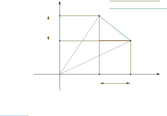
Exhibit 5.5: |
|
|
Axis 2 |
Two-dimensional illustration |
|
|
|
of the L1 (city-block) and |
|
|
|
L2 (Euclidean) distances |
|
|
|
between two points i and i': |
|
|
xi2 |
the L1 distance is the sum |
|
|
|
of the absolute differences |
|
|
|
in the coordinates, while the |
|xi2 |
– xi' 2| |
|
L2 distance is the square |
|
||
|
|
|
|
root of the sum of squared |
|
|
|
differences |
|
|
xi' 2 |
|
|
||
|
|
|
MULTIVARIATE ANALYSIS OF ECOLOGICAL DATA
L1 : dii' (1) = |xi1 – xi' 1| + |xi2 – xi' 2|
L2 : dii' (2) = (|xi1 – xi' 1|2 + |xi2 – xi' 2|2 )½
i [ xi1 xi2 ]
i' [ xi' 1 xi' 2 ]
Axis 1
xi1 |
xi' 1 |
|xi1 – xi' 1|
Dissimilarity measures for presence−absence data
In Chapter 4 we considered the matching coefficient and the chi-square distance for categorical data in general, but there is a special case which is often of interest to ecologists: presence absence, or dichotomous, data. When categorical variables have only two categories, there are a host of coefficients defined to measure inter-sample difference (see Bibliographical Appendix for references to this topic). Here we consider one example which is an alternative to the matching coefficient.
Exhibit 5.6 gives some data that we shall use again (in Chapter 7), concerning the presence absence of 10 species in 7 samples. The inter-sample differences based on the matching coefficient would be obtained either by counting the matches or mismatches between the two samples. For example, between samples A and B there are 6 matches and 4 mismatches. Usually expressed relative to the number of variables (species) this would give a similarity value of 0.6 and a dissimilarity value of 0.4. But often in ecology it is possible to have very many species in the data set, up to 100 or more, and in each sample we find relatively few of these present. This makes the number of co-absences of species very high compared to the co-presences, but both count as matches. If co-absences are not informative, we can simply ignore them and calculate similarity in terms of co-presences. Furthermore, this co-presence count is expressed not relative to the total number of species but relative to the number of species present in at least one of the two
68

MEASURES OF DISTANCE BETWEEN SAMPLES: NON-EUCLIDEAN
Exhibit 5.6:
SAMPLES |
|
|
|
|
SPECIES |
|
|
|
|
Presence−absence data of |
|
|
|
|
|
|
|
|
|
|
|
|
|
|
sp1 |
sp2 |
sp3 |
sp4 |
sp5 |
sp6 |
sp7 |
sp8 |
sp9 |
sp10 |
10 species in 7 samples |
|
|
||||||||||
|
|
|
|
|
|
|
|
|
|
|
|
A |
1 |
1 |
1 |
0 |
1 |
0 |
0 |
1 |
1 |
1 |
|
B |
1 |
1 |
0 |
1 |
1 |
0 |
0 |
0 |
0 |
1 |
|
C |
0 |
1 |
1 |
0 |
1 |
0 |
0 |
1 |
0 |
0 |
|
D |
0 |
0 |
0 |
1 |
0 |
1 |
0 |
0 |
0 |
0 |
|
E |
1 |
1 |
1 |
0 |
1 |
0 |
1 |
1 |
1 |
0 |
|
F |
0 |
1 |
0 |
1 |
1 |
0 |
0 |
0 |
0 |
1 |
|
G |
0 |
1 |
1 |
0 |
1 |
1 |
0 |
1 |
1 |
0 |
|
|
|
|
|
|
|
|
|
|
|
|
|
samples under consideration. This is the definition of the Jaccard index for dichotomous data. Taking samples A and B of Exhibit 5.6 again, the number of co-presences is 4, we ignore the 2 co-absences, then we express 4 relative to 8, so the result is 0.5. In effect, the Jaccard index is the matching coefficient of similarity calculated for a pair of samples after eliminating all the species which are co-absent. The dissimilarity between two samples is – as before – 1 minus the similarity.
Here’s another example, for samples C and D. This pair has 4 co-absences (for species 1, 7, 9 and 10), so we eliminate them. To get the dissimilarity we can count the mismatches – in fact, all the rest are mismatches – so the dissimilarity is 6/6 1, the maximum that can be attained. Using the Jaccard approach we would say that samples C and D are completely different, whereas the matching coefficient would lead to a dissimilarity of 0.6 because of the 4 matched co-absences.
To formalize these definitions, the counts of matches and mismatches in a pair of samples are put into a 2 2 table as follows:
|
Sample 2 |
|
|
|
1 |
0 |
|
1 |
|
|
|
a |
b |
a + b |
|
Sample 1 |
|
|
|
0 |
c |
d |
c + d |
|
|
|
|
|
a + c |
b + d |
a + b + c + d |
where a is the count of co-presences (1 and 1), b the count of mismatches where sample 1 has value 1 but sample 2 has value 0, and so on. The overall number of
69