

1greenacre_m_primicerio_r_multivariate_analysis_of_ecological
.pdfMULTIVARIATE ANALYSIS OF ECOLOGICAL DATA
200

INTERPRETATION, INFERENCE AND MODELLING
201
MULTIVARIATE ANALYSIS OF ECOLOGICAL DATA
202

CHAPTER 16
Variance Partitioning in PCA, LRA, CA and CCA
Principal component analysis (PCA, log-ratio analysis (LRA) and correspondence analysis (CA) form one family of methods, all based on the same mathematics of matrix decomposition and approximation by weighted least-squares. The difference between them is the type of data they are applied to, which dictates the way distances are defined between samples and between variables. In all methods there is a measure of total variance as a weighted sum of squares of the elements of a matrix that is centred or double-centred – equivalently this total variance can be defined as a weighted sum of squared distances. This total variance can be broken down into various parts, parts for each row and for each column, parts along dimensions, and parts for each row and each column along the dimensions. This neat decomposition of variance provides several diagnostics to assist in the interpretation of the solution. The same idea applies to constrained analyses such as canonical correspondence analysis (CCA), where similar decompositions take place in the constrained space.
Contents |
|
Total variance or inertia . . . . . . . . . . . . . . . . . . . . . . . . . . . . . . . . . . . . . . . . . . . . . . . . . . . . . . . . . . |
203 |
Variances on principal axes . . . . . . . . . . . . . . . . . . . . . . . . . . . . . . . . . . . . . . . . . . . . . . . . . . . . . . . |
206 |
Decomposition of principal variances into contributions . . . . . . . . . . . . . . . . . . . . . . . . . . . . . . . . . . |
206 |
Contribution coordinates . . . . . . . . . . . . . . . . . . . . . . . . . . . . . . . . . . . . . . . . . . . . . . . . . . . . . . . . . . |
208 |
Correlations between points and axes . . . . . . . . . . . . . . . . . . . . . . . . . . . . . . . . . . . . . . . . . . . . . . . |
208 |
Contributions in constrained analyses . . . . . . . . . . . . . . . . . . . . . . . . . . . . . . . . . . . . . . . . . . . . . . . |
209 |
SUMMARY: Variance partitioning in PCA, LRA, CA and CCA . . . . . . . . . . . . . . . . . . . . . . . . . . . . . . . |
211 |
PCA, LRA and CA all involve the decomposition of a matrix into parts across Total variance or inertia |
|
dimensions, from the most important dimension to the least important. Each |
|
method has a concept of total variance, also called total inertia when there are |
|
weighting factors. This measure of total variation in the data set is equal to the |
|
(weighted) sum of squared elements of the matrix being decomposed, and this |
|
total is split into parts on each ordination dimension. Let us look again at the |
|
matrix being decomposed as well as the total variance in each case. |
|
203

MULTIVARIATE ANALYSIS OF ECOLOGICAL DATA
The simplest case is that of PCA on unstandardized data, applicable to intervallevel variables that are all measured on the same scale, for example the growths in millimetres of a sample of plants during the 12 months of the year (i.e., a matrix with 12 columns), or ratio-scale positive variables that have all been log-trans- formed. Suppose that the n m cases-by-variables data matrix is X, with elements xij, then the total variance of the data set, as usually computed by most software packages, is the sum of the variances of the variables:
|
|
|
|
|
|
|
|
|
sum of variances =∑ |
1 |
|
∑ (xij |
− |
|
j )2 |
|
(16.1) |
|
x |
|||||||
|
|
|||||||
j n − 1 |
i |
|
|
|
|
|
||
Inside the square brackets is the variance of the j -th column variable of X, and these variances are summed over the columns. Since we have introduced the concept of possible row and column weightings, we often prefer to use the following definition of total variance:
total variance = |
1 |
∑ ∑ (xij − |
|
j )2 |
= |
n − 1 |
(sum of variances) |
(16.2) |
||
x |
||||||||||
|
|
|||||||||
mn |
i |
j |
|
mn |
|
|||||
That is, we divide by n and not n 1 in the variance computation, thus allocating an equal weight of 1/n to each row, and then average (rather than sum) the variances, thus allocating a weight of 1/m to each variable. So “total variance” here could rather be called average variance. This definition can easily be generalized to differential weighting of the rows and columns, so if the rows are weighted by r1, …, rn and the columns by c1, …, cm, where weights are nonnegative and sum to 1 in each case, then the total variance would be:
total variance = ∑ ∑ r c |
(x |
|
− |
|
|
)2 |
|
ij |
x |
||||||
i |
j i j |
|
|
j |
(16.3) |
||
where the variable means x j are now computed as weighted averages ∑i rixij .
When continuous variables on different scales are standardized to have variance 1, then (16.1) would simply be equal to m, the number of variables. For our averaged versions (16.2) and (16.3) would be equal to (n 1)/n, or 1 if variance is defined using 1/n times the squared deviations, rather than 1/(n 1).
In the case of LRA of a matrix N of positive values, all measured on the same scale (usually proportions or percentages) and assuming the most general case of rowand column-weighting, the data are first log-transformed to obtain a matrix
L log(N), and then double-centred using these weights. The total variance is then the weighted sum of squares of this double-centred matrix:
204

VARIANCE PARTITIONING IN PCA, LRA, CA AND CCA
total log-ratio variance = ∑ ∑ ri cj(lij − li • − l• j + l••)2 |
(16.4) |
|
i |
j |
|
where a subscript indicates weighted averaging over the respective index. An equivalent formulation is to sum the squares of all the log odds ratios in the matrix formed by a pair (i, i ) of rows and a pair (j, j ) of columns, each weighted by the respective pairs of weights:
total log-ratio variance =∑∑ ∑∑ |
|
|
nijni |
′j ′ |
|
2 |
|
||
riri ′cj cj ′ log |
|
|
(16.5) |
||||||
|
|
||||||||
i <i ′ |
j < j ′ |
|
n n |
|
|
|
|
||
|
|
|
|
|
|
|
|||
|
|
|
ij ′ i ′j |
|
|
||||
|
|
|
|
|
|
|
|||
The odds ratio is a well-known concept in the analysis of frequency data: an odds ratio of 1 is when the ratio between a pair of row elements, say, is constant across a pair of columns. For example, in the fatty acid data set of Chapter 14, when two
fatty acids j and j in two different samples i and i have the same ratio (e.g,. one is twice the other: nij /nij ni j /ni j 2), then log(1) 0 and no contribution to
the total variance is made. The higher the disparities are in comparisons of this kind, the higher is the log-ratio variance.
Finally, in CA, which applies to a table N of nonnegative variables all measured on the same scale, usually count data, the total variance (called inertia in CA jargon) is closely related to the Pearson chi-square statistic for the table. The chi-square statistic computes expected values for each cell of the table using the table margins, and measures the difference between observed and expected by summing the squared differences, each divided by the expected value:
chi-square statistic χ2 = ∑ ∑ |
(observed − expected)2 |
(16.6) |
|
|
|||
i |
j |
|
|
|
|
expected |
|
where the observed value nij and the expected value ni n j /n , and the subscript indicates summation over the respective index. The chi-square statistic increases with the grand total n of the table (which is the sample size in a crosstabulation), and the inertia in CA is a measure independent of this total. The relationship is simply as follows:
total inertia = χ2 n++ |
(16.7) |
In spite of the fact that the definitions of total variance in PCA, LRA and CA might appear to be different in their formulations, they are in fact simple variations of the same theme. Think of them as measuring the weighted dispersion of the row or column points in a multidimensional space, according to the distance
205
Variances on principal axes
MULTIVARIATE ANALYSIS OF ECOLOGICAL DATA
function particular to the method: Euclidean distance (unstandardized or standardized) for PCA, log-ratio distance for LRA and chi-square distance for CA.
The dimension-reduction step in all these methods concentrates a maximum amount of variance on the first ordination dimension, then – of the remaining variance – a maximum on the second dimension, and so on, until the last dimension, which has the least variance, in other words the dimension for which the dispersion of the rows or columns is closest to a constant. These dimensions, also called principal axes, define subspaces of best fit of the data – we are mainly interested in twodimensional subspaces for ease of interpretation. We have seen various scree plots of these parts of variance on successive dimensions (Exhibits 12.6 and 13.3), which are eigenvalues of the matrix being decomposed by each method, and usually referred to as such in program results and denoted by the Greek letter , sometimes also called principal variances or principal inertias. What we are interested in now is the decomposition of these eigenvalues into parts for each row or each column.
Decomposition of principal variances into contributions
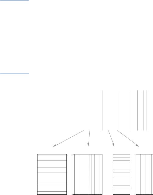
Thanks to the least-squares matrix approximation involved in this family of methods, there is a further decomposition of each ordination dimension’s variance into part contributions made by each row and each column. The complete decomposition is illustrated schematically in Exhibit 16.1. Each eigenvalue can
Exhibit 16.1: |
|
|
|
|
|
|
|
|
λ1 |
λ2 |
λ3 |
λ4 … |
|
||
Schematic explanation |
|
|
|||||
of the decomposition |
|
|
|
|
|
|
|
of total variance into |
|
|
Total variance |
|
|
|
|
parts. First, variance is |
|
|
decomposed |
|
|
|
|
decomposed from |
|
|
|
|
|
||
|
|
into parts along |
|
|
|
||
largest to smallest parts |
|
|
|
|
|
||
|
|
principal axes |
|
|
|
||
( 1, 2, …) along |
|
|
|
|
|
||
successive principal |
|
|
|
|
|
|
|
axes. Then each can |
|
|
|
|
|
|
|
be decomposed into |
|
|
|
|
|
|
|
contributions either |
|
λ1 |
λ2 |
|
etc. |
||
from the rows or from |
|
|
|||||
|
Axis 1 |
Axis 2 |
|||||
the columns. These part |
|
|
|
||||
|
|
|
|
|
|
||
contributions to each axis |
Rows |
Columns |
Rows |
Columns |
|||
provide diagnostics for |
|||||||
|
|
|
|
|
|
||
interpretation of the results
etc.
206

VARIANCE PARTITIONING IN PCA, LRA, CA AND CCA
|
dim1 |
dim2 |
dim3 |
dim4 |
Sum |
|
|
|
|
|
|
a |
0.0684 |
0.0013 |
0.0300 |
0.0025 |
0.1022 |
b |
0.0107 |
0.0202 |
0.0108 |
0.0278 |
0.0694 |
c |
0.2002 |
0.0001 |
0.0070 |
0.0012 |
0.2086 |
d |
0.0013 |
0.0000 |
0.0248 |
0.0254 |
0.0515 |
e |
0.0077 |
0.0989 |
0.0009 |
0.0045 |
0.1120 |
|
|
|
|
|
|
Sum |
0.2882 |
0.1205 |
0.0735 |
0.0614 |
0.5436 |
|
|
|
|
|
|
Exhibit 16.2:
Tabulation of the contributions of five species in data set “bioenv” to the four principal inertias of CA: the columns of this table sum to the eigenvalues (principal inertias) and the rows sum to the inertia of each species
be decomposed into parts, called contributions, either for the rows or for the columns. An example is given in Exhibit 16.2, for the CA of the “bioenv” data (see Exhibit 1.1), showing the contributions of each of the five species to the four dimensions of the CA. The grand total of this table, 0.5436, is equal to the total inertia in the data set. This is decomposed into four principal inertias, 1 0.2882,
2 0.1205, 3 0.0735, 4 0.0614 (column sums), while the values in each column are the breakdown of each principal inertia across the species. The row sums of this table are the inertias of the species themselves, and the sum of their inertias is again the total inertia.
The actual values in Exhibit 16.2 are by themselves difficult to interpret – it is easier if the rows and columns are expressed relative to their respective totals. For example, Exhibit 16.3 shows the columns expressed relative to their totals. Thus, the main contributors to dimension 1 are species a and c, accounting for 23.7% and 69.5% respectively, while species e is the overwhelming contributor to dimension 2, accounting for 82.1% of that dimension’s inertia. To single out the main contributors, we use the following simple rule of thumb: if there are 5 species, as in this example, then the main contributors are those that account for more than the average of 1/5 0.2 of the inertia on the dimension. In the last column the relative values of the inertias of each point is given when summed over all the dimensions, so that c is seen to have the highest inertia in the data matrix as a whole.
|
dim1 |
dim2 |
dim3 |
dim4 |
All |
|
|
|
|
|
|
a |
0.2373 |
0.0110 |
0.4079 |
0.0410 |
0.1880 |
b |
0.0370 |
0.1676 |
0.1463 |
0.4527 |
0.1277 |
c |
0.6947 |
0.0005 |
0.0959 |
0.0200 |
0.3837 |
d |
0.0045 |
0.0001 |
0.3373 |
0.4130 |
0.0947 |
e |
0.0266 |
0.8208 |
0.0126 |
0.0733 |
0.2060 |
|
|
|
|
|
|
Sum |
1.0000 |
1.0000 |
1.0000 |
1.0000 |
1.0000 |
|
|
|
|
|
|
Exhibit 16.3:
Contributions of the species to the principal inertias and the total inertia (Exhibit 16.2 re-expressed as values relative to column totals)
207
MULTIVARIATE ANALYSIS OF ECOLOGICAL DATA
The alternative way of interpreting the values in Exhibit 16.2 is to express each of the rows as a proportion of the row totals, as shown in Exhibit 16.4. This shows how each species’ inertia is distributed across the dimensions, or in regression terminology, how much of each species’ inertia is being explained by the dimensions as “predictors”. Because the dimensions are independent these values can be aggregated. For example, 66.9% of the inertia of species a is explained by dimension 1, and 1.3% by dimension 2, that is 68.2% by the first two dimensions. Notice in the last row of Exhibit 16.4 that the eigenvalues are also expressed relative to their total (the total inertia), showing overall how much inertia is explained by each dimension. For example, 53.0% of the total inertia of all the species is explained by dimension 1, but dimension 1 explains different percentages for each individual species: 66.9% of a, 15.4% of b, etc.
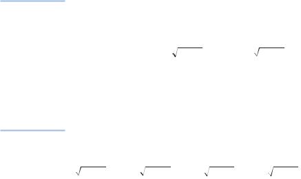
Contribution coordinates Exhibit 16.3 shows the contributions of each species to the variance of each dimension. These contributions are visualized in the contribution biplot, described in Chapter 13. Specifically, the contribution coordinates are the square roots of these values, with the sign of the respective principal or standard coordinate. For example, the absolute values of the contribution coordinates for species a on the first two dimensions are 0.2373 0.487 and 0.0110 0.105 respectively, with appropriate signs. Arguing in the reverse way, in Exhibit 13.5 the contribution coordinate on dimension 1 of the fish species Bo_sa is 0.874, hence its contribution to dimension 1 is ( 0.874)2 0.763, or 76.3%.
Correlations between points and axes
Just like the signed square roots of the contributions of points to axes in Exhibit 16.3 have a use (as contribution coordinates), so the signed square roots of the contributions of axes to points in Exhibit 16.4 also have an interesting interpretation, namely as correlations between points and axes, also called loadings in the factor analysis literature. For example, the square roots of the values for species a are
0.6690 0.818, 0.0130 0.114, 0.2934 0.542, 0.0246 0.157. These are the absolute values of the correlations of species a with axis 1, with signs depending on the sign of the respective principal or standard coordinates. Species a is thus highly correlated with axis 1, and to a lesser extent with axis 3. Remember that the four
Exhibit 16.4: |
|
|
|
|
|
|
|
|
dim1 |
dim2 |
dim3 |
dim4 |
Sum |
||
Contributions of the |
|
||||||
|
|
|
|
|
|
||
dimensions to the inertias |
a |
0.6690 |
0.0130 |
0.2934 |
0.0246 |
1.0000 |
|
of the species (Exhibit 16.2 |
b |
0.1536 |
0.2910 |
0.1550 |
0.4004 |
1.0000 |
|
re-expressed as values |
|||||||
c |
0.9600 |
0.0003 |
0.0338 |
0.0059 |
1.0000 |
||
relative to row totals). In |
|||||||
the last row the principal |
d |
0.0251 |
0.0002 |
0.4820 |
0.4928 |
1.0000 |
|
inertias are also expressed |
e |
0.0684 |
0.8832 |
0.0083 |
0.0402 |
1.0000 |
|
relative to the grand total |
|||||||
|
|
|
|
|
|
||
All |
0.5302 |
0.2216 |
0.1352 |
0.1129 |
1.0000 |
||
|
|||||||
|
|
|
|
|
|
|
208

VARIANCE PARTITIONING IN PCA, LRA, CA AND CCA
ordination dimensions function as independent predictors of the rows or columns of the data set, with the first dimension explaining the most variance, the second dimension the next highest, and so on. Each value in Exhibit 16.4 is a squared correlation and can be accumulated to give an R2 coefficient of determination, thanks to the zero correlation between the dimensions. Summing these for the first two dimensions in Exhibit 16.4 gives R2’s for the five species of 68.2%, 44.5%, 96.0%, 2.5% and 95.2% respectively – clearly, species d is very poorly explained by the first two dimensions, and from Exhibit 16.4 it is mainly explained by the last two dimensions.
In canonical correspondence analysis the dimensions are constrained to be linear combinations of external predictors. This restricts the space in which dimension reduction will take place. As seen in Chapter 15, for the “bioenv” data set, the amount of inertia in this constrained space is equal to 0.2490, compared to the 0.5436 in the unconstraineded space. This lower value of 0.2490 now becomes the total inertia that is being explained, otherwise everything is as before. Exhibit 16.5
Contributions in constrained analyses
(a) |
|
dim1 |
dim2 |
dim3 |
dim4 |
Sum |
|
|
|||||
|
|
|
|
|
|
|
|
a |
0.0394 |
0.0002 |
0.0025 |
0.0003 |
0.0424 |
|
b |
0.0131 |
0.0035 |
0.0029 |
0.0005 |
0.0201 |
|
c |
0.1470 |
0.0001 |
0.0001 |
0.0002 |
0.1474 |
|
d |
0.0000 |
0.0040 |
0.0000 |
0.0022 |
0.0061 |
|
e |
0.0013 |
0.0310 |
0.0006 |
0.0001 |
0.0330 |
|
|
|
|
|
|
|
|
Sum |
0.2008 |
0.0388 |
0.0060 |
0.0033 |
0.2490 |
(b) |
|
|
|
|
|
|
|
|
|
|
|
|
|
|
dim1 |
dim2 |
dim3 |
dim4 |
All |
|
|
|
|||||
|
|
|
|
|
|
|
|
a |
0.1962 |
0.0064 |
0.4127 |
0.0818 |
0.1703 |
|
b |
0.0652 |
0.0910 |
0.4860 |
0.1614 |
0.0807 |
|
c |
0.7321 |
0.0015 |
0.0093 |
0.0682 |
0.5919 |
|
d |
0.0001 |
0.1018 |
0.0003 |
0.6526 |
0.0247 |
|
e |
0.0063 |
0.7993 |
0.0916 |
0.0360 |
0.1324 |
|
|
|
|
|
|
|
|
Sum |
1.0000 |
1.0000 |
1.0000 |
1.0000 |
1.0000 |
(c) |
|
|
|
|
|
|
|
|
|
|
|
|
|
|
dim1 |
dim2 |
dim3 |
dim4 |
Sum |
|
|
|
|||||
|
|
|
|
|
|
|
|
a |
0.9291 |
0.0058 |
0.0587 |
0.0064 |
1.0000 |
|
b |
0.6519 |
0.1757 |
0.1459 |
0.0266 |
1.0000 |
|
c |
0.9977 |
0.0004 |
0.0004 |
0.0015 |
1.0000 |
|
d |
0.0042 |
0.6438 |
0.0003 |
0.3516 |
1.0000 |
|
e |
0.0386 |
0.9410 |
0.0168 |
0.0036 |
1.0000 |
|
|
|
|
|
|
|
|
All |
0.8066 |
0.1559 |
0.0242 |
0.0133 |
1.0000 |
|
|
|
|
|
|
|
Exhibit 16.5:
(a) Raw contributions to four dimensions by the species in the CCA of the “bioenv” data (see Chapter 15). The row sums are the inertias of the species in the restricted space, while the column sums are the principal inertias in the restricted space. (b) The contributions relative to their column sums (which would be the basis of the CCA contribution biplot. (c) The contributions relative to their row sums (i.e., squared correlations of species with axes)
209