

1greenacre_m_primicerio_r_multivariate_analysis_of_ecological
.pdfExhibit 20.7:
Scatterplots of the two FD measures versus species richness (SR, the number of species in sample), showing the modelled quadratic relationships. The horizontal axis is marked with the value of SR, and below the number of sites with the corresponding value)
MULTIVARIATE ANALYSIS OF ECOLOGICAL DATA
|
0.35 |
|
0.30 |
FD |
0.25 |
Tree-based |
0.20 |
|
0.15 |
|
0.10 |
|
0.05 |
2 |
3 |
4 |
5 |
6 |
7 |
8 |
9 |
10 |
11 |
12 |
13 |
14 |
15 |
16 |
17 |
18 |
19 |
1 |
1 |
8 |
9 |
28 |
45 |
68 |
107 |
80 |
90 |
70 |
51 |
18 |
11 |
9 |
2 |
1 |
1 |
|
1.2 |
|
1.0 |
FD |
0.8 |
Group-based |
0.6 |
|
0.4 |
|
0.2 |
|
0.0 |
2 |
3 |
4 |
5 |
6 |
7 |
8 |
9 |
10 |
11 |
12 |
13 |
14 |
15 |
16 |
17 |
18 |
19 |
1 |
1 |
8 |
9 |
28 |
45 |
68 |
107 |
80 |
90 |
70 |
51 |
18 |
11 |
9 |
2 |
1 |
1 |
270
CASE STUDY 2: FUNCTIONAL DIVERSITY OF FISH IN THE BARENTS SEA
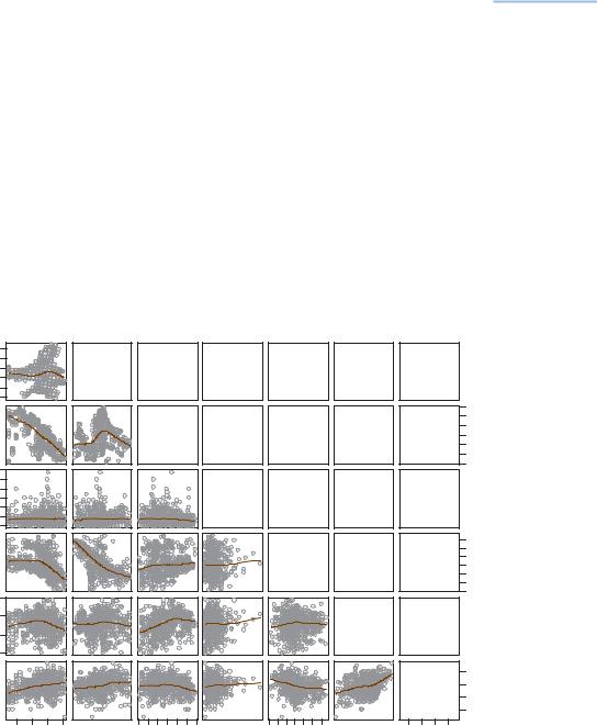
As a first bivariate view of associations between the two FD measures and the available covariates, Exhibit 20.8 shows the matrix of scatterplots, with Spearman rank correlations in the upper triangle and scatterplots and smooth relationhips in the lower triangle. Apart from the known features of the region, that depth is negatively correlated with longitude and temperature negatively correlated with latitude and longitude, the group-based FD is correlated with depth and the treebased FD negatively with temperature and positively with latitude and longitude, although these last correlations are less than 0.30 in absolute value. As already seen in Chapter 19, the variable slope does not appear to have any association with any other, so we drop it from further consideration.
To show the spatial relationship latitude and longitude should be considered together along with their interaction. We can compare two ways of spatial modelling, by spatial fuzzy coding (Chapter 11) and by generalized additive modelling (GAM,
Relating functional diversity to space, time and environment
71 |
73 |
75 |
|
0 |
10 |
20 |
30 |
|
0.0 |
1.0 |
|
|
|
|
|||||||||||||
|
|
|
|
|
|
|
|
|
|
|
|
|
|
|
|
|
|
|
|
|
|
|
|
|
|
|
30 |
Lon |
|
|
0.048 |
|
|
|
–0.63 |
|
|
0.073 |
|
|
|
–0.45 |
|
|
–0.13 |
|
0.25 |
|
|||||||
|
|
|
|
|
|
|
|
|
|
|
|
|
|
||||||||||||||
|
|
|
|
|
|
|
|
|
|
|
|
|
|
|
|||||||||||||
|
|
|
|
|
|
|
|
|
|
|
|
|
|
|
|
|
|
|
|
|
|
||||||
|
|
|
|
|
|
|
|
|
|
|
|
|
|
|
|
|
|
|
|
|
|
|
|
|
|
|
20 |
|
|
|
|
|
|
|
|
|
|
|
|
|
|
|
|
|
|
|
|
|
|
|
|
|
|
|
|
|
|
|
|
|
|
|
|
|
|
|
|
|
|
|
|
|
|
|
|
|
|
|
|
|
|
|
|
75 |
Lat |
0.25 |
|
–0.64 |
|
0.24 |
|
73 |
–0.0052 |
0.048 |
|
||||
|
|
|
|
|
|
|
|
71 |
|
|
|
|
|
|
500 |
|
|
Depth |
–0.11 |
0.093 |
0.35 |
–0.082 |
350 |
30 |
|
|
|
|
|
|
200 |
20 |
|
|
Slope |
|
0.016 |
0.12 |
|
10 |
|
|
–0.0023 |
|
|||
|
|
|
|
|
|
|
|
0 |
|
|
|
|
|
|
|
|
|
|
|
|
|
|
5 |
|
|
|
|
Temp |
0.042 |
–0.29 |
3 |
|
|
|
|
|
|||
|
|
|
|
|
|
|
1 |
|
|
|
|
|
|
|
–1 |
1.0 |
|
|
|
|
|
|
|
FDgroup |
0.30 |
|
|
|
|
|
|
|
|
|
|
|
|||
0.0 |
|
|
|
|
|
|
|
|
|
|
|
|
|
|
|
|
|
|
|
|
FDtree |
0.3 |
|
|
|
|
|
|
|
|
|
|
|
||
|
|
|
|
|
|
|
|
|
|
|
0.1 |
20 |
30 |
200 |
350 |
500 |
–1 |
1 |
3 |
5 |
0.1 |
0.3 |
|
Exhibit 20.8:
Scatterplots of the variables depth, slope, temperature, longitude and latitude
with one another as well as with the two measures of functional diversity, based on the functional groups (FDgroup) and on the dendrogram (FDtree). Spearman rank correlations are shown in the upper triangle, with font size proportional to their absolute values.
271
MULTIVARIATE ANALYSIS OF ECOLOGICAL DATA
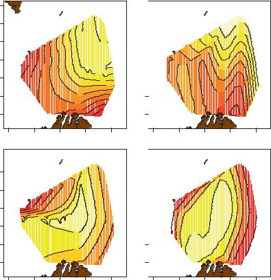
Chapter 18). For both models we model each FD measure on latitude and longitude interactively, and the results are shown in Exhibit 20.9 in the form of contours of predicted FD values.
The results or the two types of FD are quite different, with the tree-based FD showing a west and south to north-east gradient, with higher FD in the north-east, whereas the group-based FD shows higher diversity in the central area, falling off to the west and the south-east. Remember that the group-based FD takes the abundance values into account and the water in the central areas is warm, and species from more southern areas (e.g., Norwegian Sea) migrate into these areas (often in schools), especially in warmer years, giving a more equal spread of relative abundance values in the functional groups. Concerning the tree-based FD, the GAM fit shows a ridge in the diversity values from south to north while the fuzzy
Exhibit 20.9:
Contour plots of the spatial component of functional diversity according to the two definitions (first row is the tree-based FD,
second row is group-based FD) using two modelling methods (in columns, first column is using fuzzy spatial categories, second is using GAM modelling). The northern border of
Norway with Russia and the southern tip of Svalbard situate the region of interest
Fitting to fuzzy categories
|
|
77 |
|
|
|
|
76 |
|
|
FD |
Latitude |
75 |
|
|
based-Tree |
7473 |
0 |
. |
|
|
|
|
|
|
|
|
72 |
|
|
|
|
71 |
|
|
23
. |
24 |
0 |
|
25 |
|
. |
|
0 |
|
0.26
AIC = –1692
Adj R2: 14.2% 32 
 . 0
. 0
0.31
0.31 |
0.3 |
0.29 |
0.28 |
0.27 |
0.26 |
|
0.25 |
0.24 |
15 |
20 |
25 |
30 |
35 |
77

|
|
76 |
|
|
|
|
FD |
Latitude |
75 |
|
|
|
|
based-Group |
7473 |
.3 |
|
4 |
.5 |
|
|
|
|
|
. |
||
|
|
|
0 |
0 |
0 |
|
|
|
|
0.6 |
|
||
|
|
|
0.7 |
|||
|
|
|
|
|
|
0.8 |
|
|
|
|
|
|
0.9 |
AIC = 70
Adj R2: 15.8%
72 |
0.8 |
|
|
|
|
||
71 |
0.7 |
.6 |
|
0 |
|||
|
71 72 73 74 75 76 77

0 . 288
Fitting to GAM model
|
AIC = –1697 |
|
Adj R2: 15.0% |
|
.298 |
|
0 |
|
0.296 |
|
.294 |
|
0 |
|
0.29 |
0.29 |
0.292 |
|
|
|
0.288 |
|
.286 |
|
0 |
|
0.284 |
15 |
20 |
25 |
30 |
35 |
73 74 75 76 77


.8 

 0
0
|
.7 |
.65 |
0 |
|
|
0 |
|
.75 |
|
0 |
|
0.85
AIC = 123
Adj R2: 8.1%
72 |
|
|
|
|
|
|
|
71 |
.8 |
.75 |
|
7 |
0 |
. |
65 |
|
|
||||||
0 |
0. |
|
|
||||
|
0 |
|
|
|
15 |
20 |
25 |
30 |
35 |
15 |
20 |
25 |
30 |
35 |
|
|
Longitude |
|
|
|
|
Longitude |
|
|
272
CASE STUDY 2: FUNCTIONAL DIVERSITY OF FISH IN THE BARENTS SEA
fit shows a wider ridge from south-west to north-east. For the group-based FD the results are similar between the two methodological approaches, but the fuzzy approach performs noticeably better according to AIC and the adjusted R2. Another advantage of the approach using fuzzy-coded categories is that there is a p-value associated with every compass point’s difference with the central category. So we can get results that for the group-based FD several sectors are significantly lower than the central (C) one: NW, E, SE and S (all with p 0.001), NE (p 0.002) and
W (p 0.04), whereas for the tree-based FD the following sectors are significantly lower than the central one: NW (p 0.001), SE (p 0.002) and S (p 005).
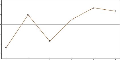
Although the spatial variation is highly linked to the variation of environmental variables such as temperature and possibly also to temporal variation, we can study inter-year variation in the residuals from the above spatial models as well as any further relationships with the environmental variables temperature and depth. As an example, we consider the residuals of tree-based classification from the fuzzy spatial model (top left example in Exhibit 20.9), and model the residuals on year as a categorical variable, and temperature and depth either as regular continuous variables, or the four-category fuzzy versions used in Chapter 19, or as smooth functions using GAM. Both temperature and depth are found to be nonsignificant predictors of the residuals, irrespective of the coding. There is significant temporal variation, however, almost identical in all analyses, which can be plotted as in Exhibit 20.10. Remembering that these are the residuals from the spatial model, we can say that in 1999 and 2001 there were lower functional diversities compared to the spatial model (as measured by the dendrogram-based approach) and higher in 2003 and 2004. All effects are different from 0 (the mean of the residuals) and highly significant (p 0.0001), apart from 2002 which is closer to 0 (p 0.025).
|
0.04 |
|
|
|
(p<0.0001) |
|
|
|
|
|
|
|
|
|
0.02 |
(p<0.0001) |
|
|
|
(p<0.0001) |
|
|
|
|
|
||
|
|
|
(p=0.025) |
|
|
|
|
|
|
|
|
|
|
effect |
0.00 |
|
|
|
|
|
Average |
–0.02 |
|
|
|
|
|
|
–0.04 |
|
(p<0.0001) |
|
|
|
|
|
|
|
|
|
|
|
(p<0.0001) |
|
|
|
|
|
|
–0.06 |
|
|
|
|
|
|
1999 |
2000 |
2001 |
2002 |
2003 |
2004 |
|
|
|
|
Years |
|
|
|
|
|
|
|
|
273 |
Exhibit 20.10:
Plot of regression coefficients for each year showing average estimated year effects for the residuals of (tree-based) functional diversities
from the spatial model, with p-values for testing differences compared to the zero mean of the residuals (dashed line)
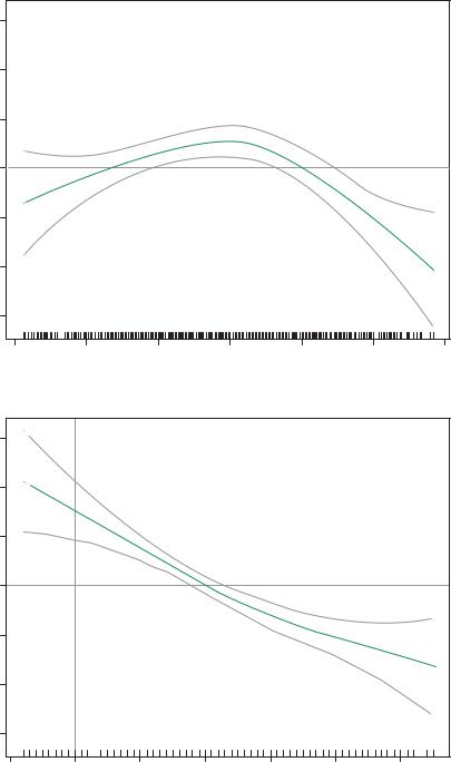
Exhibit 20.11:
GAM of tree-based FD as a smooth function of depth (p = 0.0001) and temperature (p < 0.0001). To model these effects parametrically depth would be modelled as a quadratic and temperature linear
MULTIVARIATE ANALYSIS OF ECOLOGICAL DATA
|
0.06 |
|
|
|
|
|
|
|
|
0.04 |
|
|
|
|
|
|
|
|
0.02 |
|
|
|
|
|
|
|
s(Depth, 2.73) |
0.00 |
|
|
|
|
|
|
|
|
–0.02 |
|
|
|
|
|
|
|
|
–0.06 |
|
|
|
|
|
|
|
|
200 |
250 |
300 |
350 |
|
400 |
450 |
500 |
|
|
|
|
Depth |
|
|
|
|
|
0.06 |
|
|
|
|
|
|
|
|
0.04 |
|
|
|
|
|
|
|
1.76) |
0.02 |
|
|
|
|
|
|
|
s(Temperature, |
–0.02 0.00 |
|
|
|
|
|
|
|
|
–0.06 |
|
|
|
|
|
|
|
|
–1 |
0 |
1 |
2 |
3 |
4 |
|
5 |
|
|
|
|
Temperature |
|
|
|
|
274 |
|
|
|
|
|
|
|
|

CASE STUDY 2: FUNCTIONAL DIVERSITY OF FISH IN THE BARENTS SEA
From the above it is clear that the effects of spatial position and of the environmental variables temperature and depth are confounded and difficult to separate. If FD is first related to temperature and depth, ignoring the spatial component, highly significant relationships are found: for example, tree-based FD goes down with increasing temperature and we find the same quadratic relationship with depth as in Chapter 18 where the response was species diversity – see Exhibit 18.7 for the analysis of only 89 sites (where temperature was nonsignificant), and Exhibit 20.11 for the present example of 600 sites. More or less the same depth value, about 350 m, is found here for maximum FD as was found before in Exhibit 18.7 for maximum species diversity. Adding the year effects gives almost exactly the same pattern as in Exhibit 20.9, with 1999 and 2001 low and the other years high. Of the FD variance, 30.2% (adjusted R 2) is explained by depth, temperature and years. Residuals from this environmental and temporal relationship, accounting for about 70% of the FD variance, can then be modelled spatially: using a GAM model as in Exhibit 20.8 there is still a significant spatial component in the residuals, although the explained variance in these residuals is only 4.3%.
In summary, temperature and depth, both of which are related to spatial position in the Barents Sea, are found to be strongly associated with functional diversity, and there are also significant differences between the years. Residuals from a model of FD as a function of these environmental and temporal variables can be explained, although to a minor extent, by spatial position.
1.Functional diversity measures diversity in the functional traits (feeding, motion, reproductive behaviour, habitat preferences, etc.) among species in an ecosystem.
2.Functional groups are groups of species that share the same functional traits.
3.To measure functional diversity two approaches are considered here, both based on a dendrogram obtained by hierarchical clustering of the species according to their functional traits. They are thus both dependent on the distance/dissimilarity function used as well as the type of clustering.
4.The first way is to use the hierarchical clustering to decide on the number of clusters that are sufficiently homogeneous internally to be considered separate groups. Functional diversity (FD) at a site can then be measured by any of the usual diversity measures, for example the Shannon-Weaver diversity, which is a function of relative abundances (or biomasses) of the functional groups. We call this group-based FD.
5.The second way is to add up the branches of the dendrogram of the particular mix of species at the site – this takes only presences of species into account, not their abundances. We call this tree-based FD.
SUMMARY:
Functional diversity of fish in the Barents Sea
275
MULTIVARIATE ANALYSIS OF ECOLOGICAL DATA
6.These FD measures are found to have monotonically increasing, slightly concave, relationships with species richness (SR). Tree-based FD is very closely related to SR because both take only species presences into account.
7.Both FD measures can be related to spatial, temporal and environmental variables in the usual way using multiple regression. Spatial coordinates are interactively coded to explain the spatial relationship. Continuous explanatory variables can be coded in their original form, possibly transformed to account for nonlinear relationships, or coded as fuzzy variables.
8.An alternative modelling strategy is to use generalized additive modelling (GAM) which produces a smooth regression relationship with the two-dimen- sional spatial position and the continuous variables.
276

APPENDICES
277
MULTIVARIATE ANALYSIS OF ECOLOGICAL DATA
278

APPENDIX A
Aspects of Theory
This appendix summarizes the theory described in this book. The treatment is definitely not exhaustive and the bibliography in Appendix B gives some pointers to additional reference material. We deal with the theory in more or less the same order as the corresponding methods appeared in the text, although some topics might be grouped slightly differently.
Contents
Transformations and standardization . . . . . . . . . . . . . . . . . . . . . . . . . . . . . . . . . . . . . . . . . . . . . . . . 279 Measures of distance and dissimilarity . . . . . . . . . . . . . . . . . . . . . . . . . . . . . . . . . . . . . . . . . . . . . . 281 Cluster analysis . . . . . . . . . . . . . . . . . . . . . . . . . . . . . . . . . . . . . . . . . . . . . . . . . . . . . . . . . . . . . . . . 282 Multidimensional scaling . . . . . . . . . . . . . . . . . . . . . . . . . . . . . . . . . . . . . . . . . . . . . . . . . . . . . . . . . 283 Principal component analysis, correspondence analysis and log-ratio analysis . . . . . . . . . . . . . . . . 284 Supplementary variables and points . . . . . . . . . . . . . . . . . . . . . . . . . . . . . . . . . . . . . . . . . . . . . . . . . 286 Dimension reduction with constraints . . . . . . . . . . . . . . . . . . . . . . . . . . . . . . . . . . . . . . . . . . . . . . . . 287 Permutation testing and bootstrapping . . . . . . . . . . . . . . . . . . . . . . . . . . . . . . . . . . . . . . . . . . . . . . . 288 Statistical modelling . . . . . . . . . . . . . . . . . . . . . . . . . . . . . . . . . . . . . . . . . . . . . . . . . . . . . . . . . . . . . 290
The most common measurements scales are: |
Transformations and |
|
standardization |
Continuous interval: differences between values are measured and interpreted; variables on this scale can have negative values; we also say an additive scale. For example, time, temperature.
Continuous ratio: ratios between values are measured and interpreted (i.e., percentage differences); variables on this scale have positive values; we also say a multiplicative scale. For example, heavy metal concentration, weight.
Categorical (or discrete) nominal: only a few categories are possible and they have no particular order. For example, region, phylogenetic group.
Categorical (or discrete) ordinal: only a few categories are possible and they do have an inherent ordering. For example, month, sediment class.
279