

Fig.46.6 Controllability canonical form.
We may mark distinctive features of A matrix in this scheme.
All elements of this matrix are equal to zero except for the elements located over the main diagonal (they are equal to one) and the elements of the last string.
 (46.17)
![]()
BK term for the closed-loop system will be as follows
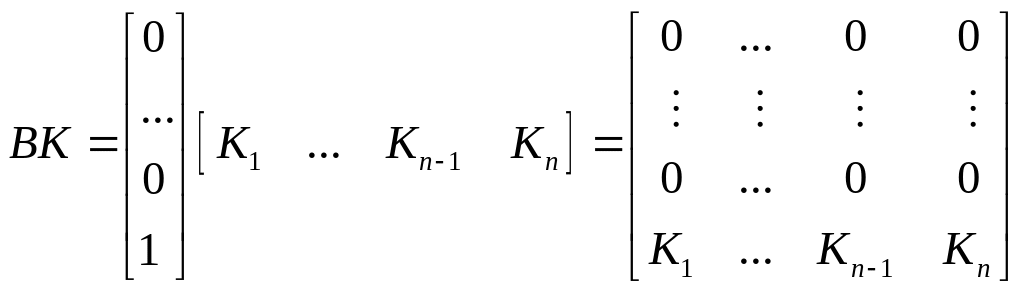
The coefficient matrix of the closed-loop system
![]() will be as follows
will be as follows
 (46.18)
This matrix is typical for controllability canonical form.
Thus, we may obtain the characteristic equation of the closed-loop control system:
![]() (46.19)
(46.19)
The desired characteristic of the closed-loop control system according to (46.14) will be as folows
![]()
Equating the coefficients for the expressions with equal powers of s in two last equations, we have
![]()
Thus, the sought coefficients are defined according to the following equation
![]() (46.20)
(46.20)
Eq.(46.20) represents the general solution of the pole placement method for SISO systems, but we have a control system complying to controllability canonical form.
But we may encounter 2 main problems:
usually state variables of the mentioned model don’t comply with natural variables of real control systems (so they don’t correspond to the physical nature of processes);
In the general case the state variables represented in controllability canonical form may be inaccessible for measurement.
The Ackermann’s formula is based on similarity
transformation, which transforms the given model with arbitrary
structure into controllability canonical
form; after that the required coefficients
![]() are defined.
are defined.
To do so we may use the Ackermann’s formula:
![]() (46.21)
(46.21)
where
![]() -
a matrix polynomial created by using the coefficients of the desired
characteristic equation
-
a matrix polynomial created by using the coefficients of the desired
characteristic equation
![]() .
.
![]() (46.22)
(46.22)
Example 46.4
Let’s consider a compensator design problem for a satellite control system.

Fig.46.7 Block diagram of a satellite control system

Fig.46.8 A simulation scheme for the satellite control system
The mentioned satellite control system has the
transfer function
![]() (look at Fig.46.7).
(look at Fig.46.7).
The state equation is as follows
![]()
Using a simulation circuit (Fig.46.8) and Eq.( 46.11) we may write:
![]() (46.23)
(46.23)
The state equations for the closed-loop system are as follows
![]()
 (46.24)
Thus, we may represent the state equations for the closed-loop system in the following form
 (46.25)
where
![]() - the coefficient matrix of the closed-loop control system.
- the coefficient matrix of the closed-loop control system.
We may define the characteristic equation of the closed-loop control system:
 (46.26)
Suppose, that design specifications require to
place the roots of characteristic equation at the points![]() .
.
In this case we may have the following desired characteristic equation:
![]() (46.27)
(46.27)
The design procedure requires to choose the
corresponding values of
![]() coefficients
in Eq.( 46.26) which are equal to the corresponding values of
coefficients in Eq.(46.27).
coefficients
in Eq.( 46.26) which are equal to the corresponding values of
coefficients in Eq.(46.27).
Thus, we may obtain:
![]() (46.28)
(46.28)
So we defined the procedure to choose corresponding feedback coefficients in order to place the roots of characteristic equation of control systems at any given points in s-plane.
If the roots of characteristic equation are
complex, then
![]() must be a complex conjugate number regarding
must be a complex conjugate number regarding![]() .
.
Example 46.5
Let’s consider a compensator design problem for a satellite control system from the previous example.
The state-space model is as follows
The desirable characteristic equation is as follows
In order to define K matrix we use the Ackermann’s formula.
![]()
then

We may define a matrix polynomial
![]()

Then we apply the Ackermann’s formula


Thus, the sought coefficient feedback matrix has the following form
![]() .
.
We obtained the result which coincides with the previous example.
Example 46.6
We continue to consider the system which controls a satellite.
Suppose, that according to requirements it’s
necessary to obtain a critically damped system with the settling time
1 s, i.e.
![]() = 1 s. Therefore the required time constant
= 1 s. Therefore the required time constant
![]() =
0.25 s, and two poles must be located at the following points s
= -4, i.e.
=
0.25 s, and two poles must be located at the following points s
= -4, i.e.
![]() =4.
=4.
In this case the desired characteristic equation will be as follows
![]()

Fig.46.9 A block diagram for the satellite control system (Example 46.6).
Объект = controlled object
Датчик скорости = speed transducer
Датчик положения = position sensor.
Fig.46.10 A simulation circuit for Example 46.6.
According to the previous example, the desired feedback coefficients are
![]() .
.
According to the simulation circuit (Fig.46.10) we may define the corresponding closed-loop transfer function
![]()

Fig.46.11 Step response characteristics of the
satellite control system to the entry conditions (![]() corresponding to
corresponding to![]() ).
).
This control system is critically damped.
Suppose, that we would like to retain the previous value of time constant = 0.25 s, but we desire to have =0.707.
It means that the roots of the characteristic
equation (the poles of the closed-loop system) must be
![]() ,
and
,
and
![]() .
.
![]() .
.
The step response characteristics are shown in Fig.46.11.
We note, that both system have the same time constant, but various values of damping factor .
You may also see Matlab script which allows to
calculate
![]() and
system response characteristic according to entry condition.
and
system response characteristic according to entry condition.
Matlab script:
A=[0 1;0 0]; B=[0;1]; C=[1 0]; D=0;
p=[-4+4i -4-4i];
K=acker(A, B, p)
sys=ss((A-B*K), B, C, D);
x0=[1 ; 0]
initial(sys,x0)
Response:
K =
32 8
