

- •Maxwell 3D User’s Guide
- •Maxwell 3D User’s Guide
- •Maxwell 3D Keyboard Shortcuts
- •User Defined Primitives
- •Maxwell and the Finite Element Method
- •The Finite Element Method in 1-D
- •The Finite Element Method in 1-D
- •The Finite Element Method in 1-D
- •The Finite Element Method in 1-D
- •3D Example: Puck Magnet above a steel plate
- •Adaptive Mesh Refinement
- •Adaptive Mesh Refinement
- •Adaptive Mesh Refinement
- •Adaptive Mesh Refinement
- •Adaptive Mesh Refinement
- •Adaptive Mesh Refinement
- •Plot of |B| on surface of the Plate (DC after 16 passes)
- •Adaptive Mesh Refinement
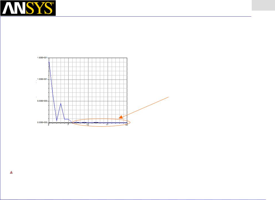
- •Plot of |B| on surface of the Plate (DC after 22 passes)
- •Convergence
- •Convergence definition through use of additional variables
- •The “Solve” Procedure in Maxwell
- •Summery
- •Example: Team Problem #20
- •Instantaneous Forces on Busbars in Maxwell 2D and 3D
- •Description
- •Setup the Design
- •Draw the Solution Region
- •Change its properties:
- •Create the Model
- •Create the Left Busbar
- •Create the Right Busbar
- •Assign the Boundaries and Sources
- •Assign the Parameters
- •Add an Analysis Setup
- •Solve the Problem
- •View the Results
- •Create a Plot of Force vs. Time
- •Setup the Design
- •Draw the Solution Region
- •Change its properties:
- •Create the Model
- •Create the Left Busbar
- •Assign the Boundaries and Sources
- •Assign the Parameters
- •Add an Analysis Setup
- •Solve the Problem
- •View the Results
- •Create a Plot of Force vs. Time
- •MSC Paper #118 "Post Processing of Vector Quantities, Lorentz Forces, and Moments
Maxwell Overview Presentation
v15 3.3
Convergence definition through use of additional variables
Delta Force [%]
Pass
Delta Force [%]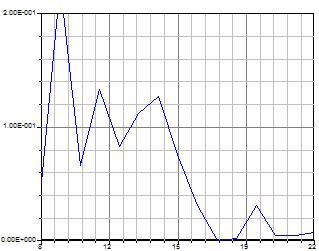
Pass
% Change in the Force on the magnet can be used to determine a more effective stopping criteria since this value can be tied directly to the acceptable numerical tolerance on a physical variable
ANSYS Maxwell Field Simulator v15 – Training Seminar |
3.3-18 |
|
|
Maxwell Overview Presentation
v15 3.3
The “Solve” Procedure in Maxwell
Start |
Generate Initial |
|
Mesh |
||
|
Solve fields using the
Finite Element Method
Calculate local |
Refine Mesh |
|
|
Solution error |
|
End criteria |
no |
reached ? |
|
yes |
|
Calculate Outputs (Force, Inductance, etc.)
ANSYS Maxwell Field Simulator v15 – Training Seminar |
3.3-19 |
|
|

Maxwell Overview Presentation
v15 3.3
Summery
Most of the execution time in a field solver is spent on the “final” solution. This is the solution that uses the largest mesh (i.e. the most finely discretized model) and hence yields the most accurate results.
Autoadaptive mesh refinement generates an efficient mesh without requiring the user to be an “expert mesher”.
User defined convergence criteria enable quantification of the trade-off between accuracy and calculation time.
|
|
|
|
|
|
|
|
ANSYS Maxwell Field Simulator v15 – Training Seminar |
3.3-20 |
||
|
|
|
|
Maxwell Overview Presentation
v15 3.3
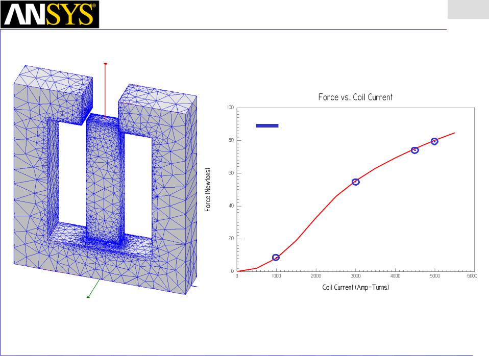
Example: Team Problem #20
Small Air Gaps
ANSYS Maxwell Field Simulator v15 – Training Seminar |
3.3-22 |
|
|
Maxwell Overview Presentation
v15 3.3
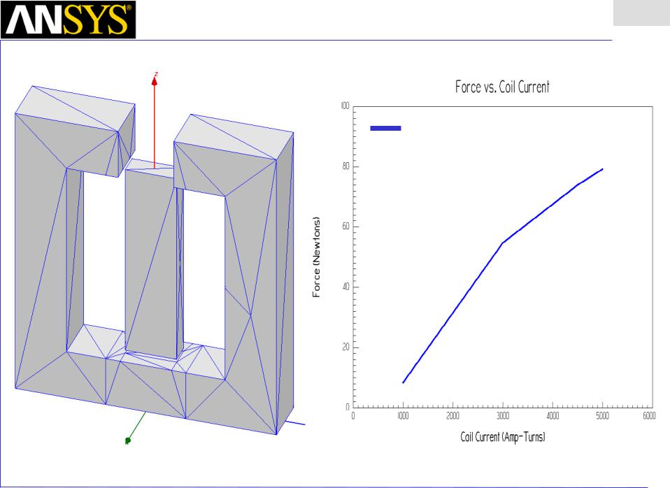
Automatic Adaptive Meshing
Measured
ANSYS Maxwell Field Simulator v15 – Training Seminar |
3.3-23 |
|
|
Maxwell Overview Presentation
v15 3.3
Comparison to Measurement
Measured
ANSYS Maxwell Field Simulator v15 – Training Seminar |
3.3-24 |
|
|

|
Maxwell v15 |
|
4.0 |
|
|
Data Reporting |
|
|
|
|
|
|
|
|
|
Overview
ANSYS Maxwell has very powerful and flexible data management and plotting capabilities. Once understood, it will make the whole solution process much easier, and will help craft the entire problem setup.
Topics of Discussion
2D Plotting
3D Plotting
Field Plotting
|
|
|
|
|
|
|
|
|
|
|
|
|
|
|
|
|
|
|
|
|
|
|
|
|
|
|
|
|
|
|
|
ANSYS Maxwell 3D Field Simulator v15 User’s Guide |
|
4.0-1 |
|||||
|
|
|
|
|
|
|
|

|
Maxwell v15 |
|
4.0 |
|
|
Data Reporting |
|
|
|
|
|
|
|
|
|
Data Plotting
Data plotting can take a variety of forms. The most often used format is 2D Cartesian plotting, but we also have the capability to plot in 3D as well. Below is a list of all the quantities that can be plotted on various graphs. For definitions of each of these quantities, see the online help or the respective solution type chapter.
Magnetostatic, Eddy Current, Electric
Force
Torque
Matrix
Transient
Motion
Position
Force/Torque
Velocity
Winding
Flux Linkage
Induced Voltage
Core Loss
Power Loss
Branch Current (external meter required)
Node Voltage (external meter required)
Fields
Mag_H
Mag_B
Mag_J
Energy Density
Coenergy Density
Apparent Energy Density
Ohmic Loss Density
Named Expressions
NOTE: For all data plots of Fields data, a Line must be defined before creating the plot.
|
|
|
|
|
|
|
|
|
|
|
|
ANSYS Maxwell 3D Field Simulator v15 User’s Guide |
|
4.0-2 |
|||
|
|
|
|
|
|
|
|
Maxwell v15 |
|
4.0 |
|
|
|
|
Data Reporting |
||
|
|
|
|
|
|
|
|
Data Plotting (Continued) |
|
|
|
|
|
|
|
|
|
|
|
|
|
|
|
|
|
Types of Plots: |
|
|
|
|
|
Rectangular Plot |
|
|
|
|
|
Data Table |
|
|
|
|
|
3D Rectangular Plot |
|
|
|
|
|
To Create a Plot: |
|
|
|
1.Select Maxwell 3D > Results > Create Magnetostatic Report
2.Reports Dialog will be displayed (options on the next page) OR
1.Select Maxwell 3D > Results > Create Fields Report
2.Reports Dialog will be displayed (options on the next page) OR
1.Select Maxwell 3D > Results > Create Quick Report (when available)
2.Choose Quick Report type and click OK.
|
|
|
|
|
|
|
|
|
|
|
|
ANSYS Maxwell 3D Field Simulator v15 User’s Guide |
|
4.0-3 |
|||
|
|
|
|
|
|

|
Maxwell v15 |
|
4.0 |
|
|
Data Reporting |
|
|
|
|
|
|
|
|
|
Data Plotting (Continued)
Creating a Plot (continued) 4. Context
Design – choose from available designs within a project
Solution – choose from available setups or solution types
Geometry – if plotting Fields data, select an available Line from the list.
5. Trace Tab
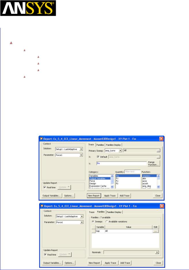
Primary Sweep – controls the source of the independent variable in the plot.
NOTE: By default, the Report editor selects Use Current Design and Project variable values. This will select the primary sweep of distance for a field data plot, or an undefined variable X for other plot types, and the current simulated values of the project variables
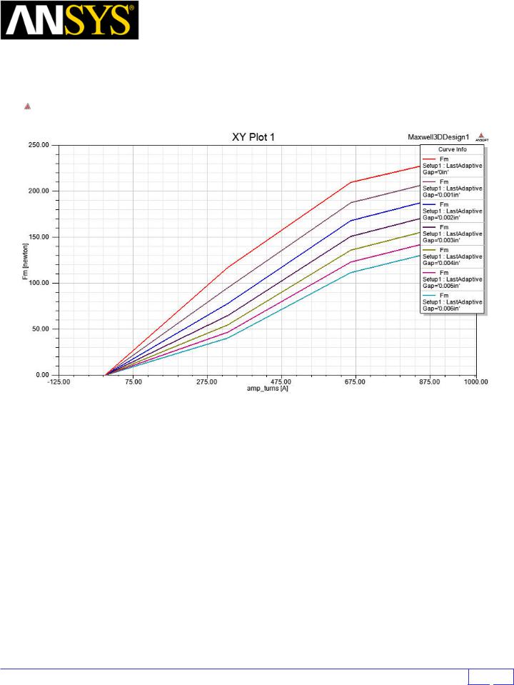
To display a plot with multiple traces for different variable values, select the Families tab and select the Sweeps for variables to be plot with. The Plot will have Primary variable as X axis and multiple traces corresponding to other variables selected from Families tab. You can also select Particular values of Sweep variable by selecting the radio button to Available variations
X – controls any functional operator on the independent variable (this is usually set to Primary Sweep).
Y – select the value to be plotted and any operator.
Category: Select the category of the variable which needs to be plot
Quantity: to Select the variable
Function: To perform arithmetic operations on variable before plot
6.
7.
Select Add Trace for as many values as you would like to plot Select Done when finished
An example of a multi-trace plot of the sweep tab shown on the previous page is shown next
|
|
|
|
|
|
|
|
|
|
|
|
ANSYS Maxwell 3D Field Simulator v15 User’s Guide |
|
4.0-4 |
|||
|
|
|
|
|
|
|
|
|
|
|
|
Maxwell v15 |
|
4.0 |
|||
|
|
|
|
|
|
|
Data Reporting |
||||
|
|
|
|
|
|
|
|
|
|
|
|
|
|
|
|
Data Plotting (Continued) |
|
|
|
|
|
||
|
|
|
|
|
|
|
|
|
|||
|
|
|
|
|
|
|
|
|
|||
|
|
|
|
|
|
|
|
|
|
|
|
|
|
|
|
|
|
|
|
|
|
|
|
|
|
|
|
|
|
|
|
|
|
|
|
|
|
|
|
|
|
|
|
|
|
|
|
|
|
|
|
|
|
|
|
|
|
|
|
|
|
|
|
|
|
|
|
|
|
|
|
|
|
|
|
|
|
|
|
|
|
|
|
ANSYS Maxwell 3D Field Simulator v15 User’s Guide |
4.0-5 |
||
|
|
|
|
|
Maxwell v15 |
|
4.1 |
|
|
Field Calculator |
|
|
|
|
|
|
|
|
|
Examples of the Field Calculator in Maxwell3D
The Field Calculator can be used for a variety of tasks, however its primary use is to extend the post-processing capabilities within Maxwell beyond the calculation / plotting of the main field quantities. The Field Calculator makes it possible to operate with primary vector fields (such as H, B, J, etc) using vector algebra and calculus operations in a way that is both mathematically correct and meaningful from a Maxwell’s equations perspective.
The Field Calculator can also operate with geometry quantities for three basic purposes:
-plot field quantities (or derived quantities) onto geometric entities;
-perform integration (line, surface, volume) of quantities over specified geometric entities;
-export field results in a user specified box or at a user specified set of locations (points).
Another important feature of the (field) calculator is that it can be fully script driven. All operations that can be performed in the calculator have a corresponding “image” in one or more lines of VBscript code. Scripts are widely used for repetitive post-processing operations, for support purposes and in cases where Optimetrics is used and post-processing scripts provide some quantity required in the optimization / parameterization process.
This document describes the mechanics of the tools as well as the “softer” side of it as well. So, apart from describing the structure of the interface this document will show examples of how to use the calculator to perform many of the post-processing operations encountered in practical, day to day engineering activity using Maxwell. Examples are grouped according to the type of solution. Keep in mind that most of the examples can be easily transposed into similar operations performed with solutions of different physical nature.
|
|
|
|
|
|
|
|
|
|
|
|
ANSYS Maxwell 3D Field Simulator v15 User’s Guide |
|
4.1-1 |
|||
|
|
|
|
|
|

|
Maxwell v15 |
|
4.1 |
|
|
Field Calculator |
|
|
|
|
|
|
|
|
|
ANSYS Maxwell Design Environment
The following features of the ANSYS Maxwell Design Environment are used to
interact with the calculator as covered in this topic
Analysis
Electrostatic
DC Conduction
Magnetostatic
Eddy Current
Transient
Results
Output Variables
Field Calculator
Field Overlays:
Named Expressions
Animate
|
|
|
|
|
|
|
|
|
|
|
|
ANSYS Maxwell 3D Field Simulator v15 User’s Guide |
|
4.1-2 |
|||
|
|
|
|
|
|

|
Maxwell v15 |
|
4.1 |
|
|
Field Calculator |
|
|
|
|
|
|
|
|
|
Description of the interface
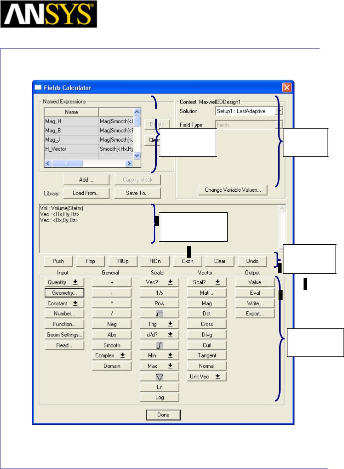
The interface is shown in Fig. I1. It is structured such that it contains a stack which holds the quantity of interest in stack registers. A number of operations are intended to allow the user to manipulate the contents of the stack or change the order of quantities being hold in stack registers. The description of the functionality of the stack manipulation buttons (and of the corresponding stack commands) is presented below:
- Push repeats the contents of the top stack register so that after the operation the two top lines contain identical information;
-Pop deletes the last entry from the stack (deletes the top of the stack);
-RlDn (roll down) is a “circular” move that makes the contents of the stacks slide down one line with the bottom of the stack advancing to the top;
-RlUp (roll up) is a “circular” move that makes the contents of the stacks slide up one line with the top of the stack dropping to the bottom;
-Exch (exchange) produces an exchange between the contents of the two top stack registers;
-Clear clears the entire contents of all stack registers;
-Undo reverses the result of the most recent operation.
The user should note that Undo operations could be nested up to the level where a basic quantity is obtained.
|
|
|
|
|
|
|
|
|
|
|
|
|
|
|
|
|
|
|
|
|
|
|
|
|
|
|
|
|
|
|
|
|
|
|
|
|
|
|
|
|
|
|
|
|
|
|
|
ANSYS Maxwell 3D Field Simulator v15 User’s Guide |
|
4.1-3 |
|||||
|
|
|
|
|
|
|
|
|
Maxwell v15 |
|
|
|
4.1 |
||
|
|
|
|
Field Calculator |
|||
|
|
|
|
|
|
|
|
|
|
|
|
|
|
|
|
|
|
|
|
|
|
|
|
|
|
|
|
|
|
|
|
Named |
Solution |
Expressions |
Context |
Stack & stack registers
Stack commands
Calculator
Buttons
Fig. I1 Field Calculator Interface
|
|
|
|
|
|
|
|
|
|
|
|
ANSYS Maxwell 3D Field Simulator v15 User’s Guide |
|
4.1-4 |
|||
|
|
|
|
|
|

|
Maxwell v15 |
|
4.1 |
|
|
Field Calculator |
|
|
|
|
|
|
|
|
|
The calculator buttons are organized in five categories as follows:
- Input contains calculator buttons that allow the user to enter data in the stack; sub-categories contain solution vector fields (B, H, J, etc.), geometry(point, line, surface, volume, coordinate system), scalar, vector or complex constants (depending on application) or even entire f.e.m. solutions.
-General contains general calculator operations that can be performed with “general” data (scalar, vector or complex), if the operation makes sense; for example if the top two entries on the stack are two vectors, one can perform the addition (+) but not multiplication (*);indeed, with vectors one can perform a dot product or a cross product but not a multiplication as it is possible with scalars.
-Scalar contains operations that can be performed on scalars; example of scalars are scalar constants, scalar fields, mathematical operations performed on vector which result in a scalar, components of vector fields (such as the X component of a vector field), etc.
-Vector contains operations that can be performed on vectors only; example of such operations are cross product (of two vectors), div, curl, etc.
-Output contains operations resulting in plots (2D / 3D), graphs, data export, data evaluation, etc.
As a rule, calculator operations are allowed if they make sense from a mathematical point of view. There are situations however where the contents of the top stack registers should be in a certain order for the operation to produce the expected result. The examples that follow will indicate the steps to be followed in order to obtain the desired result in a number of frequently encountered operations. The examples are grouped according to the type of solution (solver) used. They are typical medium/higher level post-processing task that can be encountered in current engineering practice. Throughout this manual it is assumed that the user has the basic skills of using the Field Calculator for basic operations as explained in the on-line technical documentation and/or during Ansoft basic training.
Note: The f.e.m. solution is always performed in the global (fixed) coordinate system. The plots of vector quantities are therefore related to the global coordinate system and will not change if a local coordinate system is defined with a different orientation from the global coordinate system.
|
|
|
|
|
|
|
|
|
|
|
|
|
|
|
|
|
|
|
|
|
|
|
|
|
|
|
|
|
|
|
|
ANSYS Maxwell 3D Field Simulator v15 User’s Guide |
|
4.1-5 |
|||||
|
|
|
|
|
|
|
|

|
Maxwell v15 |
|
4.1 |
|
|
Field Calculator |
|
|
|
|
|
|
|
|
|
Electrostatic Examples
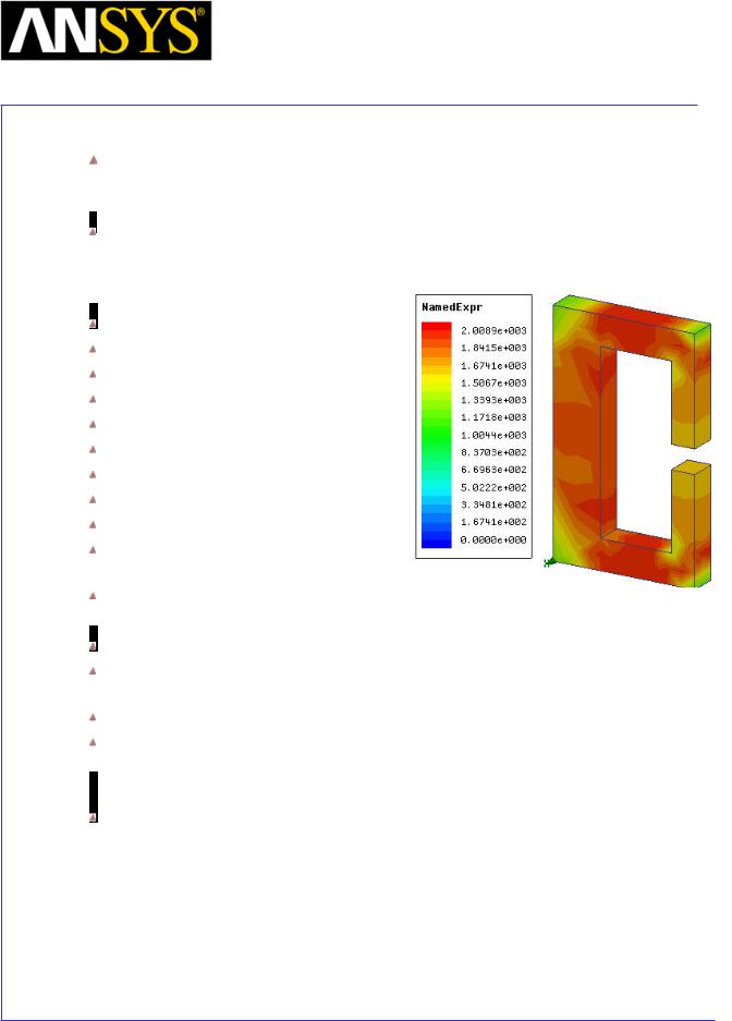
Example ES1: Calculate the charge density distribution and total electric charge on the surface of an object
Description: Assume an electrostatic (3D) application with separate metallic objects having applied voltages or floating voltages. The task is to calculate the total electric charge on any of the objects.
Calculate/plot the charge density distribution on the object; the sequence of calculator operations is described below:
Input > Quantity > D (load D vector into the calculator);
Input > Geometry
In Geometry window,
1.Select radio Button to Surface
2.Select the Surface of interest and Press OK
Vector > Unit Vec > Normal (creates the normal unit vector corresponding to the surface of interest) 
Vector > Dot (creates the dot product between D and the unit normal vector to the surface of interest, equal to the surface charge density)
Add (input “charge_density” as the name) -> OK (creates a named expression and adds it to the list)
Done (leaves calculator)
(select the surface of interest from the model)
Maxwell 3D > Fields > Fields > Named Expressions (a Selecting calculated expression window appears)
(select “charge_density” from the list) -> OK (A Create Field Plot window appears)
Done
Calculate the total electric charge on the surface of an object
Input > Quantity > D (load D vector into the calculator);
Input > Geometry > Surface… (select the surface of interest) -> OK
Vector > Normal
Scalar > ∫
Output > Eval
|
|
|
|
|
|
|
|
|
|
|
|
ANSYS Maxwell 3D Field Simulator v15 User’s Guide |
|
4.1-6 |
|||
|
|
|
|
|
|
|
Maxwell v15 |
|
|
4.1 |
|
|
|
||
|
|
|
||
|
|
|
Field Calculator |
|
|
|
|
|
|
|
|
|
|
|
Example ES2: Calculate the Maxwell stress distribution on the surface of an object
Description: Assume an electrostatic application (for ex. a parallel plate capacitor structure). The surface of interest and adjacent region should have a fine finite element mesh since the Maxwell stress method for calculation the force is quite sensitive to mesh.
The Maxwell electric stress vector has the following expression for objects without electrostrictive effects:
TnE = (D n)E − 12 nεE 2
where the unit vector n is the normal vector to the surface of interest. The sequence of calculator commands necessary to implement the above formula is given below.
Input > Quantity > D
Input > Geometry > Surface (select the surface of interest) > OK
Vector > Unit Vec > Normal (creates the normal unit vector corresponding to the surface of interest)
Vector > Dot
Input > Quantity > E
General > * (multiply)
Input > Geometry > Surface… (select the surface of interest) > OK
Vector > Unit Vec > Normal (creates the normal unit vector corresponding to the surface of interest)
Input > Number >Scalar (0.5) OK General > *
Input > Constant > Epsi0 General > *
Input > Quantity > E Push
Dot General > *
General > - (minus) Continued on next page.
|
|
|
|
|
|
|
|
|
|
|
|
ANSYS Maxwell 3D Field Simulator v15 User’s Guide |
|
4.1-7 |
|||
|
|
|
|
|
|
|
Maxwell v15 |
|
4.1 |
|
|
Field Calculator |
|
|
|
|
|
|
|
|
|
Example ES2: Continued
Add … (input “stress” as the name) > OK (creates a named expression and adds it to the list)
Done (leaves calculator)
(select the surface of interest from the model)
Maxwell 3D > Fields > Fields > Named Expressions (a Selecting calculated expression window appears)
(select “stress” from the list) > OK (A Create Field Plot window appears) Done
If an integration of the Maxwell stress is to be performed over the surface of interest, then use the Named Expression in the following calculator sequence:
(select “stress” from the Named Expressions list)
Copy to stack (inserts the named expression to the stack)
Input > Geometry > Surface (select surface of interest) > OK
Vector > Normal
Scalar > ∫
Output > Eval
Note: The surface in all the above calculator commands should lie in free space or should coincide with the surface of an object surrounded by free space (vacuum, air). It should also be noted that the above calculations hold true in general for any instance where a volume distribution of force density is equivalent to a surface distribution of stress (tension):
F = ∫ fdv =  ∫Tn dS
vΣ Σ
where Tn is the local tension force acting along the normal direction to the surface and F is the total force acting on object(s) inside Σ.
The above results for the electrostatic case hold for magnetostatic applications if the electric field quantities are replaced with corresponding magnetic quantities.
|
|
|
|
|
|
|
|
|
|
|
|
ANSYS Maxwell 3D Field Simulator v15 User’s Guide |
|
4.1-8 |
|||
|
|
|
|
|
|
|
Maxwell v15 |
|
|
4.1 |
|
|
|
||
|
|
|
||
|
|
|
Field Calculator |
|
|
|
|
|
|
|
|
|
|
|
Current flow Examples
Example CF1: Calculate the resistance of a conduction path between two terminals
Description: Assume a given conductor geometry that extends between two terminals with applied DC currents.
In DC applications (static current flow) one frequent question is related to the calculation of the resistance when one has the field solution to the conduction (current flow) problem. The formula for the analytical calculation of the DC
resistance is:
RDC = C∫σ(s)dsA(s)
where the integral is calculated along curve C (between the terminals) coinciding with the “axis” of the conductor. Note that both conductivity and cross section area are in general function of point (location along C). The above formula is not easily implementable in the general case in the field calculator so that alternative methods to calculate the resistance must be found.
One possible way is to calculate the resistance using the power loss in the respective conductor due to a known conduction current passing through the conductor.
|
|
P |
|
|
|
|
|
|
|
|
|||||
|
RDC = |
|
where power loss is given by P = ∫V |
E J dV = ∫ |
J |
J dV |
|
|
I DC2 |
||||||
|
σ |
||||||
|
|
|
|
|
V |
|
|
The sequence of calculator commands to compute the power loss P is given below:
Input > Quantity > J Push
Input > Number > Scalar (1e7) OK (conductivity assumed to be 1e7 S/m) General > / (divide)
Vector > Dot
Input > Geometry > Volume (select the volume of interest) > OK Scalar > ∫
Output > Eval
The resistance can now be easily calculated from power and the square of the current.
Continued on next page.
|
|
|
|
|
|
|
|
|
|
|
|
ANSYS Maxwell 3D Field Simulator v15 User’s Guide |
|
4.1-9 |
|||
|
|
|
|
|
|

|
Maxwell v15 |
|
|
4.1 |
|
|
|
||
|
|
|
||
|
|
|
Field Calculator |
|
|
|
|
|
|
|
|
|
|
|
There is another way to calculate the resistance which makes use of the well
known Ohm’s law.
RDC = UI
Assuming that the conductor is bounded by two terminals, T1 and T2 (current through T1 and T2 must be the same), the resistance of the conductor (between T1 and T2) is given the ratio of the voltage differential U between T1 and T2 and the respective current, I . So it is necessary to define two points on the respective terminals and then calculate the voltage at the two locations (voltage is called Phi in the field calculator). The rest is simple as described above.
Example CF2: Export the field solution to a uniform grid
Description: Assume a conduction problem solved. It is desired to export the field solution at locations belonging to a uniform grid to an ASCII file.
The field calculator allows the field solutions to be exported regardless of the nature of the solution or the type of solver used to obtain the solution. It is possible to export any quantity that can be evaluated in the field calculator. Depending on the nature of the data being exported (scalar, vector, complex), the structure of each line in the output file is going to be different. However, regardless of what data is being exported, each line in the data section of the output file contains the coordinates of the point (x, y, z) followed by the data being exported (1 value for a scalar quantity, 2 values for a complex quantity, 3 values for a vector in 3D, 6 values for a complex vector in 3D)
Continued on next page.
|
|
|
|
|
|
|
|
|
|
|
|
ANSYS Maxwell 3D Field Simulator v15 User’s Guide |
|
4.1-10 |
|||
|
|
|
|
|
|
|
Maxwell v15 |
|
4.1 |
|
|
Field Calculator |
|
|
|
|
|
|
|
|
|
To export the current density vector to a grid the field calculator steps are:
Input > Quantity > J
Output > Export (then fill in the data as appropriate, see Fig. CF2)
OK
Fig. CF2 Define the size of the export region (box) and spacing within
Select Calculate grid points and define minimum, maximum & spacing in all 3 directions X, Y, Z as the size of the rectangular export region (box) and the spacing between locations. By default the location of the ASCII file containing the export data is in the project directory. Clicking on the browse symbol one can also choose another location for the exported file.
Note: One can export the quantity calculated with the field calculator at user specified locations by selecting Input grid points from file. In that case the ASCII file containing on each line the x, y and z coordinates of the locations must exist prior to initiating the export-to-file command.
|
|
|
|
|
|
|
|
|
|
|
|
ANSYS Maxwell 3D Field Simulator v15 User’s Guide |
|
4.1-11 |
|||
|
|
|
|
|
|

|
Maxwell v15 |
|
4.1 |
|
|
Field Calculator |
|
|
|
|
|
|
|
|
|
Example CF3: Calculate the conduction current in a branch of a complex conduction path
Description: There are situations where the current splits along the conduction path. If the nature of the problem is such that symmetry considerations cannot be applied, it may be necessary to evaluate total current in 2 or more parallel branches after the split point. To be able to perform the calculation described above, it is necessary to have each parallel branch (where the current is to be calculated) modeled as a separate solid.
Before the calculation process is started, make sure that the (local) coordinate system is placed somewhere along the branch where the current is calculated, preferably in a median location along that branch. In more general terms, that location is where the integration is performed and it is advisable to choose it far from areas where the current splits or changes direction, if possible.
Here is the process to be followed to perform the calculation using the field calculator.
Input > Quantity > J
Input > Geometry > Volume (choose the volume of the branch of interest) OK
General > Domain (this is to limit the subsequent calculations to the branch of interest only)
Input > Geometry > Surface > yz (choose axis plane that cuts perpendicular to the branch) OK
Vector > Normal Scalar > ∫ Output > Eval
The result of the evaluation is positive or negative depending on the general orientation of the J vector versus the normal of the integration surface (S). In mathematical terms the operation performed above can be expressed as:
I = ∫J n dS
S
Note: The integration surface (yz, in the example above) extends through the whole region, however because of the “domain” command used previously, the calculation is restricted only to the specified solid (that is the S surface is the intersection between the specified solid and the integration plane).
|
|
|
|
|
|
|
|
|
|
|
|
ANSYS Maxwell 3D Field Simulator v15 User’s Guide |
|
4.1-12 |
|||
|
|
|
|
|
|

|
Maxwell v15 |
|
4.1 |
|
|
Field Calculator |
|
|
|
|
|
|
|
|
|
Magnetostatic examples
Example MS1: Calculate (check) the current in a conductor using Ampere’s theorem
Description: Assume a magnetostatic problem where the magnetic field is produced by a given distribution of currents in conductors. To calculate the current in the conductor using Ampere’s theorem, a closed polyline (of arbitrary shape) should be drawn around the respective conductor. In a mathematical form the Ampere’s theorem is given by:
ISΓ =  ∫H ds
∫H ds
Γ
where Γ is the closed contour (polyline) and SΓ is an open surface bounded by Γ but otherwise of arbitrary shape. ISΓ is the total current intercepting the surface SΓ.
To calculate the (closed) line integral of H, the sequence of field calculator commands is: 
Input > Quantity > H
Input > Geometry > Line (choose the closed polygonal line around the conductor) OK
Vector > Tangent Scalar > ∫ Output > Eval
The value should be reasonably close to the value of the corresponding current. The match between the two can be used as a measure of the global accuracy of the calculation in the general region where the closed line was placed.
|
|
|
|
|
|
|
|
|
|
|
|
ANSYS Maxwell 3D Field Simulator v15 User’s Guide |
|
4.1-13 |
|||
|
|
|
|
|
|

|
Maxwell v15 |
|
|
4.1 |
|
|
|
||
|
|
|
||
|
|
|
Field Calculator |
|
|
|
|
|
|
|
|
|
|
|
Example MS2: Calculate the magnetic flux through a surface
Description: Assume the case of a magnetostatic application. To calculate the magnetic flux through an already existing surface the sequence of calculator commands is:
Input > Quantity > B
Input > Geometry > Surface (specify the integration surface) OK
Vector > Normal
Scalar > ∫
Output > Eval
The result is positive or negative depending on the orientation of the B vector with respect to the normal to the surface of integration.
The above operation corresponds to the following mathematical formula for the magnetic flux:
ΦS = ∫B n dA
S
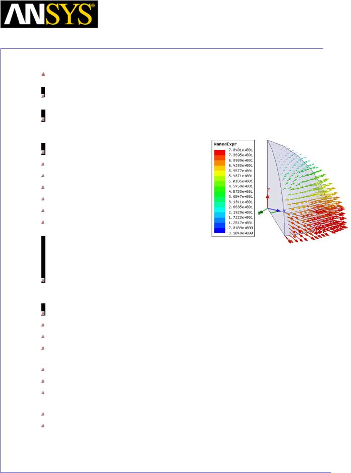
Example MS3: Calculate components of the Lorentz force
Description: Assume a distribution of magnetic field surrounding conductors with applied DC currents. The calculation of the components of the Lorentz force has the following steps in the field calculator.
Input > Quantity > J
Input > Quantity > B
Vector > Cross
Vector > Scal? > ScalarX
Input > Geometry > Volume (specify the volume of interest) OK
Scalar > ∫
Output > Eval
The above example shows the process for calculating the X component of the Lorentz force. Similar steps should be performed for all components of interest.
|
|
|
|
|
|
|
|
|
|
|
|
ANSYS Maxwell 3D Field Simulator v15 User’s Guide |
|
4.1-14 |
|||
|
|
|
|
|
|
|
Maxwell v15 |
|
4.1 |
|
|
Field Calculator |
|
|
|
|
|
|
|
|
|
Example MS4: Calculate the distribution of relative permeability in nonlinear material
Description: Assume a non-linear magnetostatic problem. To plot the relative permeability distribution inside a non-linear material the following steps should be taken:
Input > Quantity > B Vector > Scal? > ScalarX Input > Quantity > H Vector > Scal? > ScalarX Input > Constant > Mu0 General > * (multiply) General > / (divide) General > Smooth
Add (input “rel_perm” as the name)
OK (creates a named expression and adds it to the list)
Done (leaves calculator)
(select the surface of interest from the model)
Maxwell 3D > Fields > Fields > Named Expressions (a Selecting calculated expression window appears)
(select “rel_perm” from the list) > OK (a Create Field Plot window appears) Done
Note: The above sequence of commands makes use of one single field component (X component). Please note that any spatial component can be used for the purpose of calculating relative permeability in isotropic, non-linear soft magnetic materials. The result would still be the same if we used the Y component or the Z component. However, this does not apply for anisotropic materials. The “smoothing” also used in the sequence is also recommended particularly in cases where the mesh density is not very high.
|
|
|
|
|
|
|
|
|
|
|
|
ANSYS Maxwell 3D Field Simulator v15 User’s Guide |
|
4.1-15 |
|||
|
|
|
|
|
|
|
Maxwell v15 |
|
|
4.1 |
|
|
|
||
|
|
|
||
|
|
|
Field Calculator |
|
|
|
|
|
|
|
|
|
|
|
Frequency domain (AC) Examples
Example AC1: Calculate the radiation resistance of a circular loop
Description: Assume a circular loop of radius 0.02 m with an applied current excitation at 1.5 GHz;
The radiation resistance is given by the following formula:
Rr = |
Pav |
P |
= |
1 |
∫∫S |
Re(E × H * )dS = |
1 |
∫∫S |
Re |
1 |
( × H )× H * dS |
|
2 |
||||||||||||
2 |
2 |
|
||||||||||
|
Irms |
av |
|
|
jωε0 |
|
||||||
|
|
|
|
|
|
|
|
|
|
|||
where S is the outer surface of the region (preferably spherical), placed conveniently far away from the source of radiation.
Assuming that a half symmetry model is used, no ½ is needed in the above formula. The sequence of calculator commands necessary for the calculation of the average power is as follows:
Input > Quantity > H
Vector > Curl
Input > Number > Complex (0 , -12) OK
General > *
Input > Quantity > H
General > Complex > Conj
Vector > Cross
General > Complex > Real
Input > Geometry > Surface (select the surface of interest) > OK
Vector > Normal
Scalar > ∫
Output > Eval
Note: The integration surface above must be an open surface (radiation surface) if a symmetry model is used. Surfaces of existing objects cannot be used since they are always closed. Therefore the necessary integration surface must be created in the example above using Modeler > Surface > Create Object From Face command.
|
|
|
|
|
|
|
|
|
|
|
|
ANSYS Maxwell 3D Field Simulator v15 User’s Guide |
|
4.1-16 |
|||
|
|
|
|
|
|
|
Maxwell v15 |
|
4.1 |
|
|
Field Calculator |
|
|
|
|
|
|
|
|
|
Example AC2: Calculate/Plot the Poynting vector
Description: Same as in Example AC1.
To obtain the Poynting vector the following sequence of calculator commands is necessary:
Input > Quantity > H
Vector > Curl
Input > Number > Complex (0 , -12) OK
General > *
Input > Quantity > H
General > Complex > Conj
Vector > Cross
To plot the real part of the Poynting vector the following commands should be added to the above sequence:
General > Complex > Real
Input > Number > Scalar (0.5) OK General > *
Add (input “Poynting” as the name) > OK (creates a named expression and adds it to the list)
Done (leaves calculator)
(select the surface of interest from the model)
Maxwell 3D > Fields > Fields > Named Expressions (a Selecting calculated expression window appears)
(select “Poynting” from the list) > OK (a Create Field Plot window appears) Done
|
|
|
|
|
|
|
|
|
|
|
|
|
|
|
|
|
|
|
|
|
|
|
|
|
|
|
|
|
|
|
|
ANSYS Maxwell 3D Field Simulator v15 User’s Guide |
|
4.1-17 |
|||||
|
|
|
|
|
|
|
|
|
Maxwell v15 |
|
4.1 |
|
|
Field Calculator |
|
|
|
|
|
|
|
|
|
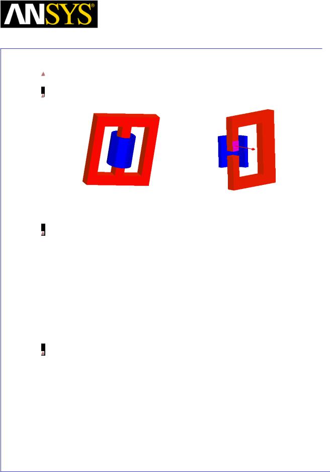
Example AC3: Calculate total induced current in a solid
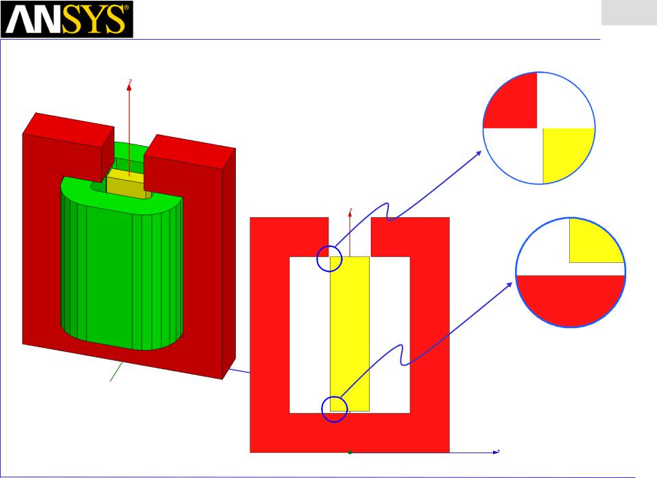
Description: Consider (as example) the device in Fig. AC3.
|
a) full model |
b) quarter model |
|
Fig. AC3 Geometry of inductor model
Assume that the induced current through the surface marked with an arrow in the quarter model is to be calculated. Please note that there is an expected net current flow through the market surface, due to the symmetry of the problem. As a general recommendation, the surface that is going to be used in the process of integrating the current density should exist prior to solving the problem. In some cases this also means that the geometry needs to be created in such a way so that the particular post-processing task is made possible. Once the object containing the integration surface exists, use the Modeler > Surface > Create Object From Face command to create the integration surface necessary for the calculation. Make sure that the object with expected induced currents has non-zero conductivity and that the eddy-effect calculation was turned on.
Assuming now that all of the above was taken care of, the sequence of calculator commands necessary to obtain separately the real part and the imaginary part of the induced current is described on the next page:
|
|
|
|
|
|
|
|
|
|
|
|
|
|
|
|
|
|
|
|
|
|
|
|
|
|
|
|
|
|
|
|
ANSYS Maxwell 3D Field Simulator v15 User’s Guide |
|
4.1-18 |
|||||
|
|
|
|
|
|
|
|

|
Maxwell v15 |
|
|
4.1 |
|
|
|
||
|
|
|
||
|
|
|
Field Calculator |
|
|
|
|
|
|
|
|
|
|
|
For the real part of the induced current:
Input > Quantity > J General > Complex > Real
Input > Geometry > Surface (select previously defined integration surface) OK Vector > Normal
Scalar > ∫ Output > Eval
For the imaginary part of the induced current:
Input > Quantity > J General > Complex > Imag
Input > Geometry > Surface (select previously defined integration surface) OK Vector > Normal
Scalar > ∫
Output > Eval
If instead of getting the real and imaginary part of the current , one desires to do an “at phase” calculation, the sequence of commands is:
Input > Quantity > J
Input > Number > Scalar (45) OK (assuming a calculation at 45 degrees phase angle)
General > Complex > AtPhase
Input > Geometry > Surface (select previously defined integration surface) OK Vector > Normal
Scalar > ∫
Output > Eval
|
|
|
|
|
|
|
|
|
|
|
|
|
|
|
|
|
|
|
|
|
|
|
|
|
|
|
|
|
|
|
|
ANSYS Maxwell 3D Field Simulator v15 User’s Guide |
|
4.1-19 |
|||||
|
|
|
|
|
|
|
|

|
Maxwell v15 |
|
4.1 |
|
|
Field Calculator |
|
|
|
|
|
|
|
|
|
Example AC4: Calculate (ohmic) voltage drop along a conductive path
Description: Assume the existence of a conductive path (a previously defined open line totally contained inside a conductor). To calculate the real and imaginary components of the ohmic voltage drop inside the conductor the following steps should be followed:
For the real part of the voltage:
Input > Quantity > J
Vector > Matl > Conductivity > Divide OK
General > Complex > Real
Input > Geometry > Line > (select the applicable line) OK
Vector > Tangent
Scalar > ∫
Output > Eval
For the imaginary part of the voltage:
Input > Quantity > J
Vector > Matl > Conductivity > Divide OK
General > Complex > Imag
Input > Geometry > Line > (select the applicable line) OK
Vector > Tangent
Scalar > ∫
Output > Eval
To calculate the phase of the voltage manipulate the contents of the stack so that the top register contains the real part of the voltage and the second register of the stack contains the imaginary part. To calculate phase enter the following command:
Scalar > Trig > Atan2
|
|
|
|
|
|
|
|
|
|
|
|
ANSYS Maxwell 3D Field Simulator v15 User’s Guide |
|
4.1-20 |
|||
|
|
|
|
|
|
|
Maxwell v15 |
|
|
4.1 |
|
|
|
||
|
|
|
||
|
|
|
Field Calculator |
|
|
|
|
|
|
|
|
|
|
|
Example AC5: Calculate the AC resistance of a conductor
Description: Consider the existence of an AC application containing conductors with significant skin effect. Assume also that the mesh density is appropriate for the task, i.e. mesh has a layered structure with 1-2 layers per skin depth for 3-4 skin depths if the conductor allows it. Here is the sequence to follow in order to calculate the total power dissipated in the conductor of interest.
Input > Quantity > OhmicLoss
Input > Geometry > Volume (specify volume of interest) OK Scalar > ∫
Output > Eval
Note: To obtain the AC resistance the power obtained above must be divided by the squared rms value of the current applied to the conductor. Note that in the Boundary/Source Manager peak values are entered for sources, not rms values.
|
|
|
|
|
|
|
|
|
|
|
|
ANSYS Maxwell 3D Field Simulator v15 User’s Guide |
|
4.1-21 |
|||
|
|
|
|
|
|

|
Maxwell v15 |
|
|
4.1 |
|
|
|
||
|
|
|
||
|
|
|
Field Calculator |
|
|
|
|
|
|
|
|
|
|
|
Time Domain Examples
Example TD1: Plotting Transient Data
Description: Assume a time domain (transient application) requiring the display of induced current as a function of time. Do this before solving if fields are not saved at every step, or any time if fields are available.
Input > Quantity > J
Input > Geometry > Surface (enter the surface of interest) OK Vector > Normal
Scalar > ∫
Add (input “Induced_Current” as the name) > OK (creates a named expression and adds it to the list)
Done (leaves calculator)
Maxwell 3D > Results > Output Variables… (an Output Variables Dialogue appears)
(select Fields from the Report Type pull down menu)
(select Calculator Expressions as the Category and “Induced_Current” as the Quantity)
Insert Quantity Into Expression
(name your expression by writing “Ind_Cur” in the Name textbox)
Add (adds an output variable and its expression to the list) Done
This Output Variable can be accessed two ways. First, it can be accessed directly in the reports - make sure that the Reports Type is set to Fields (not Transient). Second, it can be included in the Solve setup under the Output Variables tab (which also makes it available in the reports with the Reports Type set to Transient).
|
|
|
|
|
|
|
|
|
|
|
|
ANSYS Maxwell 3D Field Simulator v15 User’s Guide |
|
4.1-22 |
|||
|
|
|
|
|
|

|
Maxwell v15 |
|
4.1 |
|
|
Field Calculator |
|
|
|
|
|
|
|
|
|
Example TD2: Find the maximum/minimum field value/location
Description: Consider a solved transient application. To find extreme field values in a given volume and/or the respective locations follow these steps.
To get the value of the maximum magnetic flux density in a given volume:
Input > Quantity > B
Vector > Mag
Input > Geometry > Volume (enter volume of interest) OK
Scalar > Max > Value
Output > Eval
To get the location of the maximum:
Input > Quantity > B
Vector > Mag
Input > Geometry > Volume (enter volume of interest) OK
Scalar > Max > Position
Output > Eval
The process is very similar when searching for the minimum. Just replace the Max with Min in the above sequences.
|
|
|
|
|
|
|
|
|
|
|
|
ANSYS Maxwell 3D Field Simulator v15 User’s Guide |
|
4.1-23 |
|||
|
|
|
|
|
|

|
Maxwell v15 |
|
4.1 |
|
|
Field Calculator |
|
|
|
|
|
|
|
|
|
Example TD3: Combine (by summation) the solutions from two time steps
Description: Assume a linear model transient application. It is possible to add the solution from different time steps if you follow these steps:
First, set the solution context to a certain time step, say t1 by selecting View > Set Solution Context… and choosing an appropriate time from the list.
Then in the calculator:
Input > Quantity > B
Write (enter the name of the file) OK
Exit the calculator and choose a different time step, say t2.
Then, in the calculator:
Input > Quantity > B
Read (specify the name of the .reg file to be read in) OK
General > + (add)
Vector > Mag
Input > Geometry > Surface > (enter surface of interest) OK
Note 1: For this operation to succeed it is necessary that the respective meshes are identical. This condition is of course satisfied in transient applications without motion since they do not have adaptive meshing. It should be noted that this capability can be used in other solutions sequences –say staticif the meshes in the two models are identical.
The whole operation is numeric entirely, therefore the nature of the quantities being “combined” is not checked from a physical significance point of view. It is possible to add for example an H vector solution to a B vector solution. This doesn’t have of course any physical significance, so the user is responsible for the physical significance of the operation.
For the particular case of time domain applications it is possible to study the “displacement” of the (vector) solution from one time step to another, study the spatial orthogonality of two solution, etc. It is a very powerful capability that can be used in many interesting ways.
|
|
|
|
|
|
|
|
|
|
|
|
ANSYS Maxwell 3D Field Simulator v15 User’s Guide |
|
4.1-24 |
|||
|
|
|
|
|
|
|
Maxwell v15 |
|
4.1 |
|
|
Field Calculator |
|
|
|
|
|
|
|
|
|
Example TD3: Continued
Note 2: As another example of using this capability please consider another typical application: power flow in a given device.
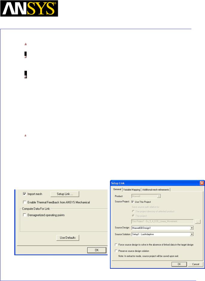
As example one can consider the case of a cylindrical conductor above the ground plane with 1 Amp current, the voltage with respect to the ground being 1000 V. As well known, one can solve separately the magnetostatic problem (in which case the voltage is of no consequence, and only magnetic fields are calculated) and the electrostatic problem (in which case only the electric fields are calculated). With Maxwell it is possible to “combine” the two results in the post-processing phase if the assumption that the electric and magnetic fields are totally separated and do not influence each other. One possible reason that such an operation is meaningful from a physical point of view might be the need for an analysis of power flow.
Assume that a magnetostatic and electrostatic problem are created with identical geometries. Link the mesh from one simulation to the mesh of the other, so that they will be identical – this can be accomplished in the Setup tab of the Analysis Setup properties. Select the Import mesh box, and clicking on the Setup Link … button. Then specify the target Design and Solution in the Setup Link dialog. To assure that the mesh is identical in both the linked solution and the target solution, make sure to set the Maximum Number of Passes to one (1) in the linked solution.
|
|
|
|
|
|
|
|
|
|
|
|
|
|
|
|
|
|
|
|
|
|
|
|
|
|
|
|
|
|
|
|
|
|
|
|
|
|
|
|
|
|
|
|
|
|
|
|
|
|
|
|
|
|
|
|
|
|
|
|
ANSYS Maxwell 3D Field Simulator v15 User’s Guide |
|
4.1-25 |
|||||||
|
|
|
|
|
|
|
|
|
|

|
Maxwell v15 |
|
4.1 |
|
|
Field Calculator |
|
|
|
|
|
|
|
|
|
Example TD3: Continued
Solve both these models and access the electrostatic results. Export the electric field solution as follows:
Input > Quantity > E
Output > Write… (enter the name of the .reg file to contain the solution) OK
Access now the solution of the magnetostatic problem and perform the following operations with the calculator after placing the coordinate system in the median plane of the conductor (yz plane if the conductor is oriented along x axis):
Input > Read (specify the name of the file containing electrostatic E field) OK Input > Quantity > H
Vector > Cross
Input > Geometry > Volume > background > OK General > Domain
Input > Geometry > Surface > yz Vector > Normal
Scalar > ∫
Output > Eval
A result around 1000 W should be obtained, corresponding to 1000 W of power being transferred along the wire but NOT THROUGH THE WIRE! Indeed the power is transmitted through the air around the wire (the Poynting vector has higher values closer to the wire and decays in a radial direction). The wire here only has the role of GUIDING the power transfer! The wire absorbs from the electromagnetic field only the power corresponding to the conduction losses in the wire.
When the integration of the Poynting vector was performed above, a domain operation was also performed limiting the result to the background only. This shows clearly that the distribution of the Poynting vector in the background is responsible for the power transfer. Displaying the Poynting vector in different transversal planes to the wire shows also the direction of the power transfer.
This type of analysis can be very useful in studying the power transfer in complex devices.
|
|
|
|
|
|
|
|
|
|
|
|
ANSYS Maxwell 3D Field Simulator v15 User’s Guide |
|
4.1-26 |
|||
|
|
|
|
|
|

|
Maxwell v15 |
|
4.1 |
|
|
Field Calculator |
|
|
|
|
|
|
|
|
|
Example TD4: Create an animation from saved field solutions
Description: Assume a solved time domain application. To create an animation file of a certain field quantity extracted from the saved field solution (say magnitude of conduction current density J) proceed as described below.
(select surface of interest)
Maxwell 3D > Fields > Fields > J > Mag_J
Done
Maxwell 3D > Fields > Animate … (a Setup Animation dialogue appears)
(select desired time steps from those available in the list)
Done
|
|
|
|
|
|
|
|
|
|
|
|
ANSYS Maxwell 3D Field Simulator v15 User’s Guide |
|
4.1-27 |
|||
|
|
|
|
|
|

|
Maxwell v15 |
|
4.1 |
|
|
Field Calculator |
|
|
|
|
|
|
|
|
|
Miscellaneous Examples
Example M1: Calculation of volumes and areas
To calculate the volume of an object here is the sequence of calculator commands:
Input > Number > Scalar (1) OK (enters the scalar value of 1)
Input > Geometry > Volume (enter the volume of interest) OK
Scalar > ∫
Output > Eval
The result is expressed in m3.
To calculate the area of a surface here is the sequence of calculator commands:
Input > Number > Scalar (1) OK (enters the scalar value of 1)
Input > Geometry > Surface (enter the surface of interest) OK
Scalar > ∫
Output > Eval
The result is expressed in m2.
|
|
|
|
|
|
|
|
|
|
|
|
ANSYS Maxwell 3D Field Simulator v15 User’s Guide |
|
4.1-28 |
|||
|
|
|
|
|
|

|
Maxwell v15 |
|
5.0 |
|
Chapter 5.0 – Magnetostatic |
|
|
|
|
|
|
|
|
|
|
Chapter 5.0 – Magnetostatic Examples
5.1 – Magnetic Force
5.2 – Inductance Calculation
5.3 –Stranded Conductors
5.4 – Equivalent Circuit Extraction (ECE) Linear Movement
5.5 – Anisotropic Materials
5.6 – Symmetry Boundaries
5.7 – Permanent Magnet Magnetization 5.8 – Master/Slave boundaries
|
|
|
|
|
|
|
|
|
|
|
|
|
|
|
|
|
|
|
|
|
|
|
|
|
|
|
|
|
|
|
|
|
|
|
|
|
|
|
|
|
|
|
|
|
|
|
|
|
|
|
|
|
|
|
|
|
|
|
|
ANSYS Maxwell 3D Field Simulator v15 User’s Guide |
|
5.0 |
|
||||||
|
|
|
|
|
|
|
|
|
|
Maxwell v15 |
5.1 |
Example (Magnetostatic) – Magnetic Force
Magnetic Force
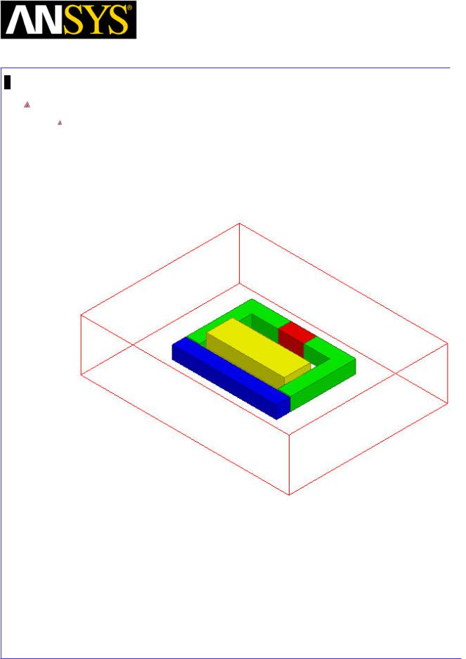
This example is intended to show you how to create and analyze a magnetostatic problem with a permanent magnet to determine the force exerted on a steel bar using the Magnetostatic solver in the Ansoft Maxwell 3D Design Environment.
|
|
|
|
|
|
|
|
|
|
|
|
|
|
|
|
|
|
|
|
|
|
|
|
|
|
|
|
|
|
|
|
|
|
|
|
|
|
|
|
|
|
|
|
|
|
|
|
|
|
|
|
|
|
|
|
|
|
|
|
ANSYS Maxwell 3D Field Simulator v15 User’s Guide |
|
5.1-1 |
|||||||
|
|
|
|
|
|
|
|
|
|
Maxwell v15 |
5.1 |
Example (Magnetostatic) – Magnetic Force
ANSYS Maxwell Design Environment
The following features of the ANSYS Maxwell Design Environment are used to
create the models covered in this topic
3D Solid Modeling
Primitives: Box
Surface Operations: Section
Boolean Operations: Subtract, Unite, Separate Bodies
Boundaries/Excitations
Current: Stranded
Analysis
Magnetostatic
Results
Force
Field Overlays:
Vector B
|
|
|
|
|
|
|
|
|
|
|
|
|
|
|
|
|
|
|
|
|
|
|
|
|
|
|
|
|
|
|
|
ANSYS Maxwell 3D Field Simulator v15 User’s Guide |
|
5.1-2 |
|||||
|
|
|
|
|
|
|
|

Maxwell v15 |
5.1 |
Example (Magnetostatic) – Magnetic Force
Launching Maxwell
To access Maxwell:
1.Click the Microsoft Start button, select Programs, and select Ansoft > Maxwell 15.0 and select Maxwell 15.0
Setting Tool Options
To set the tool options:
Note: In order to follow the steps outlined in this example, verify that the following tool options are set :
1. Select the menu item Tools > Options > Maxwell 3D Options
Maxwell Options Window:
1. Click the General Options tab
Use Wizards for data input when creating new boundaries: Checked
Duplicate boundaries/mesh operations with geometry:
Checked
2.Click the OK button
2.Select the menu item Tools > Options > Modeler Options.
Modeler Options Window:
1. Click the Operation tab
 Automatically cover closed polylines: Checked 2. Click the Display tab
 Default transparency = 0.8 3. Click the Drawing tab
 Edit property of new primitives: Checked 4. Click the OK button
|
|
|
|
|
|
|
|
|
|
|
|
|
|
|
|
|
|
|
|
|
|
|
|
|
|
|
|
|
|
|
|
ANSYS Maxwell 3D Field Simulator v15 User’s Guide |
|
5.1-3 |
|||||
|
|
|
|
|
|
|
|

Maxwell v15 |
5.1 |
Example (Magnetostatic) – Magnetic Force
Opening a New Project
To open a new project:
After launching Maxwell, a project will be automatically created. You can also create a new project using below options.
1.In an Maxwell window, click the On the Standard toolbar, or select the menu item File > New.
Select the menu item Project > Insert Maxwell 3D Design, or click on the icon
Set Solution Type
To set the Solution Type:
Select the menu item Maxwell 3D > Solution Type
Solution Type Window:
1.Choose Magnetostatic
2.Click the OK button
|
|
|
|
|
|
|
|
|
|
|
|
|
|
|
|
|
|
|
|
|
|
|
|
|
|
|
|
|
|
|
|
|
|
|
|
|
|
|
|
|
|
|
|
|
|
|
|
|
|
|
|
|
|
|
|
|
|
|
|
ANSYS Maxwell 3D Field Simulator v15 User’s Guide |
|
5.1-4 |
|||||||
|
|
|
|
|
|
|
|
|
|
Maxwell v15 |
5.1 |
Example (Magnetostatic) – Magnetic Force
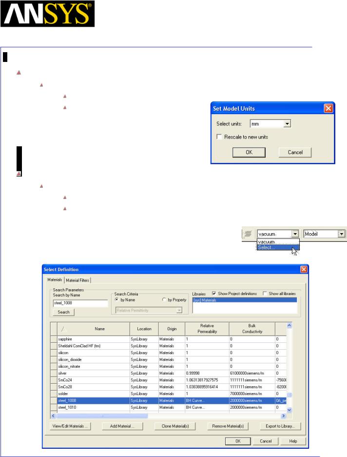
Set Model Units
To Set the units:
Select the menu item Modeler > Units
Set Model Units:
1.Select Units: mm
2.Click the OK button
Set Default Material
To set the default material:
Using the 3D Modeler Materials toolbar, choose Select
In Select Definition window,
1.Type steel_1008 in the Search by Name field
2.Click the OK button
|
|
|
|
|
|
|
|
|
|
|
|
|
|
|
|
|
|
|
|
|
|
|
|
|
|
|
|
|
|
|
|
ANSYS Maxwell 3D Field Simulator v15 User’s Guide |
|
5.1-5 |
|||||
|
|
|
|
|
|
|
|
Maxwell v15 |
5.1 |
Example (Magnetostatic) – Magnetic Force
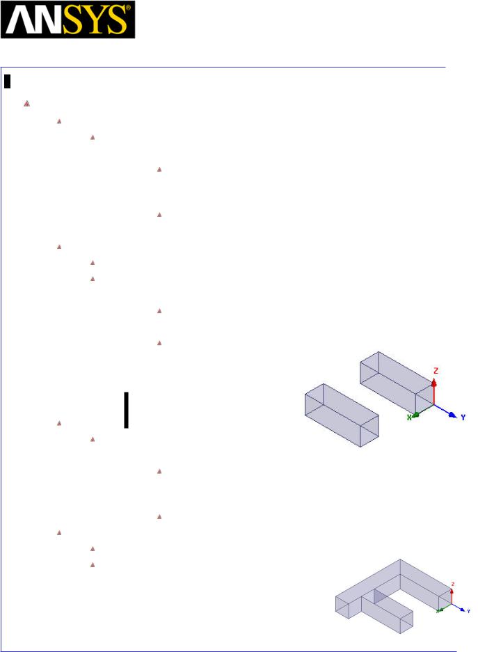
Create Core
Create Box
Select the menu item Draw > Box
1. Using the coordinate entry fields, enter the box position X: 0, Y: 0, Z: -5, Press the Enter key
2.Using the coordinate entry fields, enter the opposite corner of the box:
dX: 10, dY: -30, dZ: 10, Press the Enter key
 Select the menu item View > Fit All > Active View. Duplicate Box
Select the object Box1 from the history tree
Select the menu item Edit > Duplicate Along Line
Using the coordinate entry fields, enter the first point
X: 0, Y: 0, Z: 0, Press the Enter key
Using the coordinate entry fields, enter the second point dX: 30, dY: 0, dZ: 0, Press the Enter key
3.Total Number: 2
4.Click the OK button
Create another box
Select the menu item Draw > Box
1. Using the coordinate entry fields, enter the box position X: 0, Y: -30, Z: -5, Press the Enter key
2.Using the coordinate entry fields, enter the opposite corner of the box:
dX: 50, dY: -10, dZ: 10, Press the Enter key
Unite Objects
Select the menu item Edit > Select All
Select the menu item, Modeler > Boolean > Unite
|
|
|
|
|
|
|
|
|
|
|
|
|
|
|
|
|
|
|
|
|
|
|
|
|
|
|
|
|
|
|
|
|
|
|
|
|
|
|
|
|
|
|
|
|
|
|
|
|
|
ANSYS Maxwell 3D Field Simulator v15 User’s Guide |
|
5.1-6 |
|||||||
|
|
|
|
|
|
|
|
|
|
Maxwell v15 |
5.1 |
Example (Magnetostatic) – Magnetic Force
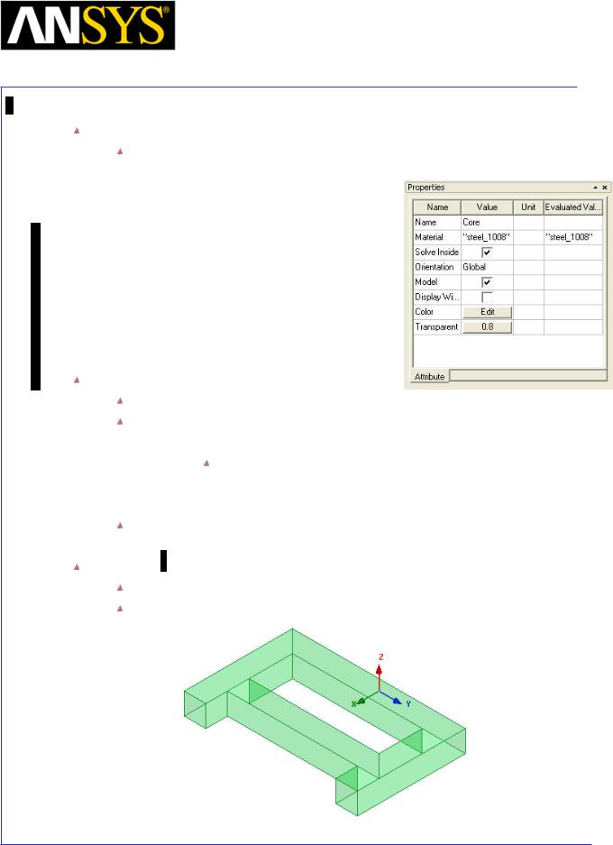
Change Attributes
Select the resulting object from the tree and goto Properties window
1.Change the name of the object to Core
2.Change its color to Green
Mirror object
Select the Object Core from the history tree
Select the menu item, Edit > Duplicate > Mirror
1. Using the coordinate entry fields, enter the first point
X: 0, Y: 0, Z: 0, Press the Enter key
2. Using the coordinate entry fields, enter the normal point
 dX: 0, dY: 1, dZ: 0, Press the Enter key Select the menu item View > Fit All > Active View.
Unite Objects
Press Ctrl and select the objects Core and Core_1 from the history tree
Select the menu item, Modeler > Boolean > Unite
|
|
|
|
|
|
|
|
|
|
|
|
|
|
|
|
|
|
|
|
|
|
|
|
|
|
|
|
|
|
|
|
|
|
|
|
|
|
|
|
|
|
|
|
|
|
|
|
|
|
|
|
|
|
|
|
|
|
|
|
|
|
|
|
|
|
|
|
|
|
|
|
|
|
|
|
|
|
|
|
|
|
|
|
|
|
|
|
|
|
|
|
|
|
|
|
ANSYS Maxwell 3D Field Simulator v15 User’s Guide |
|
5.1-7 |
|||||||||
|
|
|
|
|
|
|
|
|
|
|
|
Maxwell v15 |
5.1 |
Example (Magnetostatic) – Magnetic Force
Create Bar
Create Box
Select the menu item Draw > Box
1. Using the coordinate entry fields, enter the box position X: 51, Y: -40, Z: -5, Press the Enter key
2.Using the coordinate entry fields, enter the opposite corner of the box:
dX: 10, dY: 80, dZ: 10, Press the Enter key
Change Attributes
Select the object from the tree and goto Properties window
1.Change the name of the object to Bar
2.Change its color to Blue
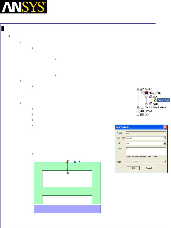
Parameterize Object
Expand the history tree of the object Bar
Double click on the command CreateBox from the tree
For Position, type: 50mm+mx, -40, -5, Click the Tab key to accept
In Add variable window,
1.Unit Type: Length
2.Unit: mm
3.Value: 1
4.Press OK
Press OK to exit
|
|
|
|
|
|
|
|
|
|
|
|
|
|
|
|
|
|
|
|
|
|
|
|
|
|
|
|
|
|
|
|
|
|
|
|
|
|
|
|
|
|
|
|
|
|
|
|
|
|
ANSYS Maxwell 3D Field Simulator v15 User’s Guide |
|
5.1-8 |
|||||||
|
|
|
|
|
|
|
|
|
|
Maxwell v15 |
5.1 |
Example (Magnetostatic) – Magnetic Force
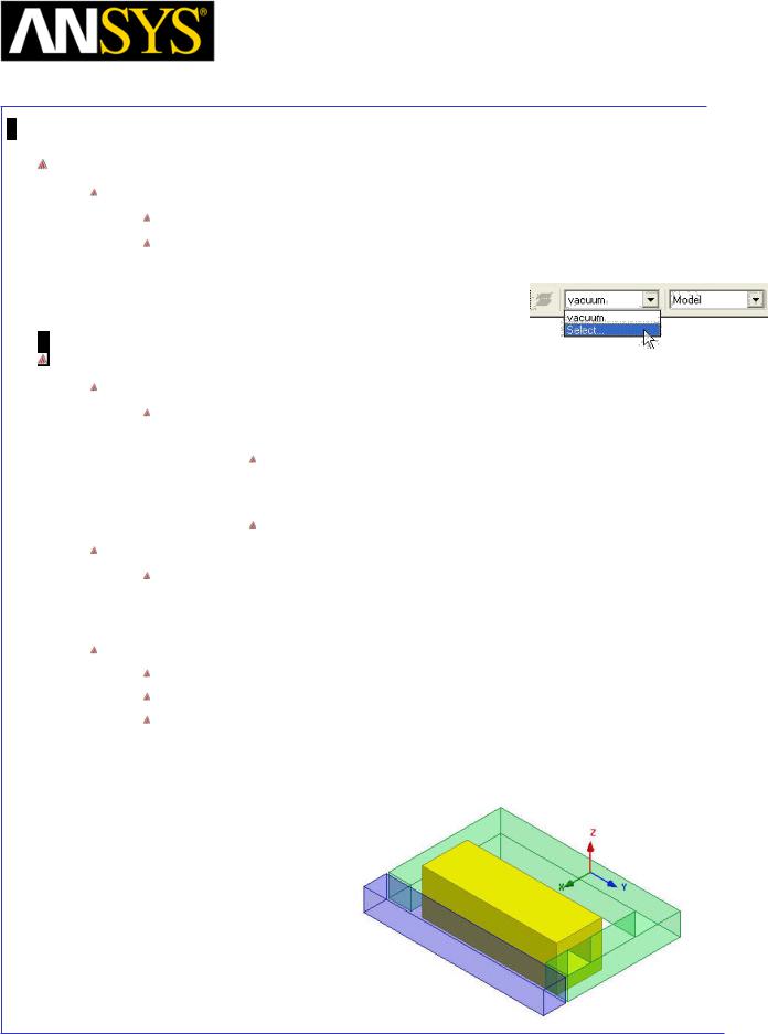
Set Default Material
To set the default material:
Using the 3D Modeler Materials toolbar, choose Select
In Select Definition window,
1.Type Copper in the Search by Name field
2.Click the OK button
Create Coil
Create Box
Select the menu item Draw > Box
1. Using the coordinate entry fields, enter the box position X: 45, Y: 30, Z: 10, Press the Enter key
2.Using the coordinate entry fields, enter the opposite corner of the box:
dX: -20, dY: -60, dZ: -20, Press the Enter key
Change Attributes
Select the object from the tree and goto Properties window
1.Change the name of the object to Coil
2.Change its color to Yellow
Subtract Core
Press Ctrl and select the objects Core and Coil from the history tree
Select the menu item Modeler > Boolean > Subtract
In Subtract Window,
1.Blank Parts: Coil
2.Tool Parts: Core
3.Clone tool objects before subtracting: Checked
4.Click the OK button
|
|
|
|
|
|
|
|
|
|
|
|
|
|
|
|
|
|
|
|
|
|
|
|
|
|
|
|
|
|
|
|
|
|
|
|
|
|
|
|
|
|
|
|
|
|
|
|
|
|
|
|
|
|
|
|
|
|
|
|
|
|
|
|
|
|
|
|
|
|
|
|
|
|
|
|
|
|
|
|
|
|
|
|
ANSYS Maxwell 3D Field Simulator v15 User’s Guide |
|
5.1-9 |
|||||||||
|
|
|
|
|
|
|
|
|
|
|
|
Maxwell v15 |
5.1 |
Example (Magnetostatic) – Magnetic Force
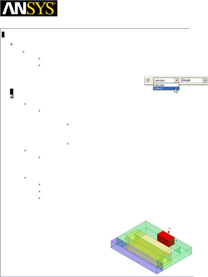
Set Default Material
To set the default material:
Using the 3D Modeler Materials toolbar, choose Select
In Select Definition window,
1.Type NdFe35 in the Search by Name field
2.Click the OK button
Create Magnet
Create Box
Select the menu item Draw > Box
1. Using the coordinate entry fields, enter the box position X: 0, Y: -10, Z: -5, Press the Enter key
2.Using the coordinate entry fields, enter the opposite corner of the box:
dX: 10, dY: 20, dZ: 10, Press the Enter key
Change Attributes
Select the object from the tree and goto Properties window
1.Change the name of the object to Magnet
2.Change its color to Red
Subtract Object
Press Ctrl and select the objects Magnet and Core from the history tree
Select the menu item Modeler > Boolean > Subtract
In Subtract Window
1.Blank Parts: Core
2.Tool Parts: Magnet
3.Clone tool objects before subtracting: Checked
4.Click the OK button
|
|
|
|
|
|
|
|
|
|
|
|
|
|
|
|
|
|
|
|
|
|
|
|
|
|
|
|
|
|
|
|
|
|
|
|
|
|
|
|
|
|
|
|
|
|
|
|
|
|
ANSYS Maxwell 3D Field Simulator v15 User’s Guide |
|
5.1-10 |
|||||||
|
|
|
|
|
|
|
|
|
|
Maxwell v15 |
5.1 |
Example (Magnetostatic) – Magnetic Force
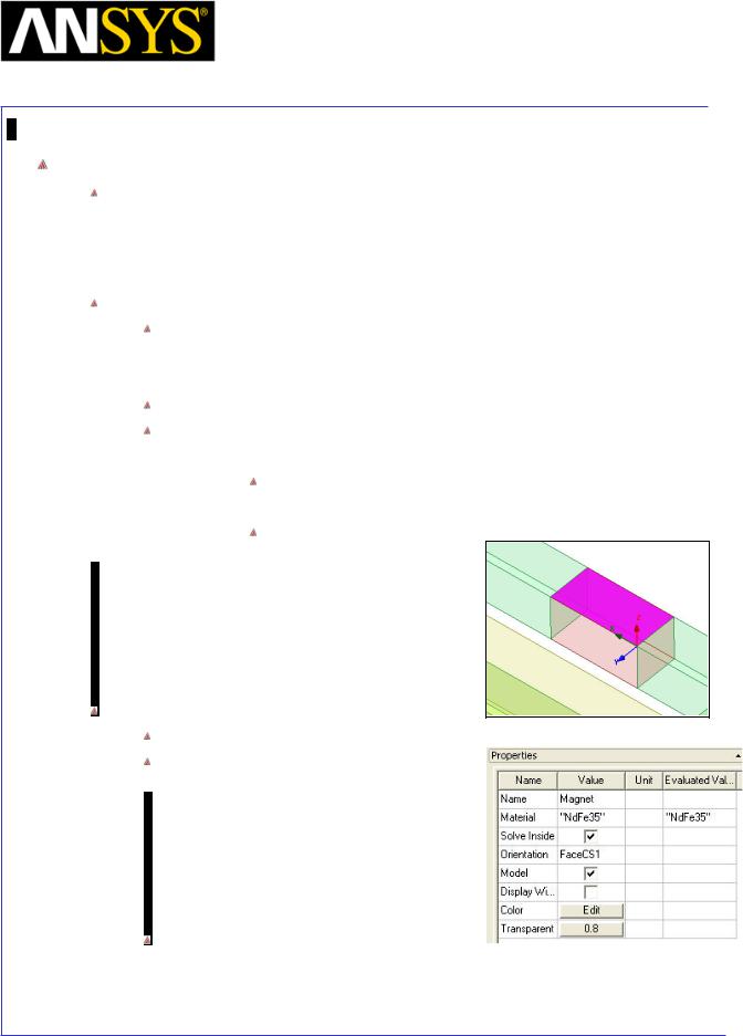
Orient Magnet
Note: By default all objects in Maxwell will have their orientation with respect to global co-ordinate system and all magnetic materials are magnetized in X direction. If actual direction of magnetization is different from Global axis, we need to create Local coordinate system in that direction and orient the magnet with respect to local coordinate system.
Create Local coordinate system
Change Selection from Object to faces
1.Select the menu item Edit > Select > Faces or
2.Press shortcut key “F” from keyboard
Using the mouse, select the top face of the Magnet from graphic window Select the menu item Modeler > Coordinate System > Create > Face CS
1. Using the coordinate entry fields, enter the origin
X: 10, Y: 10, Z: 5, Press the Enter key
2. Using the coordinate entry fields, enter the axis: dX: 0, dY: -20, dZ: 0, Press the Enter key
Change Orientation of Magnet
Select Magnet from the tree and goto Properties window
Change Orientation to FaceCS1
Change Selection to Objects
1.Select the menu item Edit > Select > Objects or
2.Press shortcut key “O” from keyboard
|
|
|
|
|
|
|
|
|
|
|
|
ANSYS Maxwell 3D Field Simulator v15 User’s Guide |
|
5.1-11 |
|||
|
|
|
|
|
|
Maxwell v15 |
5.1 |
Example (Magnetostatic) – Magnetic Force
Assign Boundaries
Assign Insulating boundary to prevent current leakage out of the Coil
Select the object Coil from the tree
Select the menu item Maxwell 3D > Boundaries > Assign > Insulating
In Insulating Boundary window,
1.Name: Insulating1
2.Click the OK button
Create Excitations
Change Work Coordinate System
Goto Modeler > Coordinate System > Set Working CS
In Select Coordinate System Window
1.Select Global
2.Press Select
Create Section of coil for assigning Current
Select the object Coil from the history tree
Select the menu item Modeler > Surface > Section
In Section window,
1.Section Plane: XY
2.Click the OK button
Change Attributes
Select the object Coil_Section1 from the tree and goto Properties window 1. Change the name of the object to Coil_Terminal
Separate Sheets
Select the sheet Coil_Terminal
Select the menu item Modeler > Boolean > Separate Bodies
Delete Extra Sheets
Select the sheet Coil_Terminal_Seperate1 from the tree Select the menu item Edit >Delete
|
|
|
|
|
|
|
|
|
|
|
|
|
|
|
|
|
|
|
|
|
|
|
|
|
|
|
|
|
|
|
|
ANSYS Maxwell 3D Field Simulator v15 User’s Guide |
|
5.1-12 |
|||||
|
|
|
|
|
|
|
|
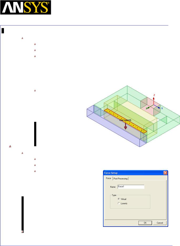
Maxwell v15 |
5.1 |
Example (Magnetostatic) – Magnetic Force
Assign Excitations
Select the sheet Coil_Terminal from the history tree
Select the menu item Maxwell 3D > Excitations > Assign > Current
In Current Excitation window,
1.Name: Current1
2.Value: c1
3.Type: Stranded
4.Current Direction: negative Z (Use Swap Direction if needed)
5.Press OK
In Add variable window,
1.Unit Type: Current
2.Unit: A
3.Value: 100
4.Press OK
Create Force Parameter
Create Parameter to calculate Force
Select the Object Bar from the history tree
Select the menu item Maxwell 3D > Parameters > Assign > Force
In Force Setup window,
1.Name: Force1
2.Type: Virtual
3.Press OK button
Note: Virtual forces are useful on any object while Lorentz forces are only applicable on current carrying objects which have permeability = 1.
|
|
|
|
|
|
|
|
|
|
|
|
ANSYS Maxwell 3D Field Simulator v15 User’s Guide |
|
5.1-13 |
|||
|
|
|
|
|
|
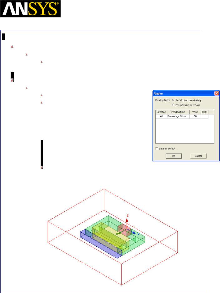
Maxwell v15 |
5.1 |
Example (Magnetostatic) – Magnetic Force
Set Default Material
To Set Default Material
Using the 3D Modeler Materials toolbar, choose Vacuum
Define Region
Create Simulation Region
Select the menu item Draw > Region
In Region window,
1.Pad all directions similarly: Checked
2.Padding Type: Percentage Offset
3.Value: 50
4.Press OK
Note: For all Maxwell 3D projects a solution space must be defined. Unless a partial model (like a motor wedge) is used, a region is usually created as described above.
|
|
|
|
|
|
|
|
|
|
|
|
|
|
|
|
|
|
|
|
|
|
|
|
|
|
|
|
|
|
|
|
ANSYS Maxwell 3D Field Simulator v15 User’s Guide |
|
5.1-14 |
|||||
|
|
|
|
|
|
|
|
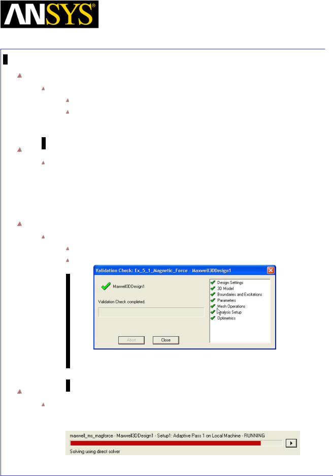
Maxwell v15 |
5.1 |
Example (Magnetostatic) – Magnetic Force
Analysis Setup
To create an analysis setup:
Select the menu item Maxwell 3D > Analysis Setup > Add Solution Setup
Solution Setup Window:
1. Click the OK button to accept all default settings.
Save Project
To save the project:
1.In an Ansoft Maxwell window, select the menu item File > Save As.
2.From the Save As window, type the Filename: Ex_5_1_Magnetic_Force
3.Click the Save button
Model Validation
To validate the model:
Select the menu item Maxwell 3D > Validation Check
Click the Close button
Note: To view any errors or warning messages, use the Message Manager.
Analyze
To start the solution process:
1. Select the menu item Maxwell 3D > Analyze All
|
|
|
|
|
|
|
|
|
|
|
|
|
|
|
|
|
|
|
|
|
|
|
|
|
|
|
|
|
|
|
|
ANSYS Maxwell 3D Field Simulator v15 User’s Guide |
|
5.1-15 |
|||||
|
|
|
|
|
|
|
|
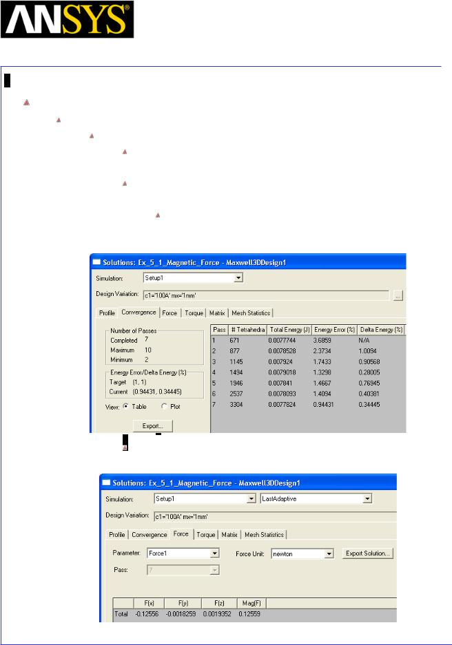
Maxwell v15 |
5.1 |
Example (Magnetostatic) – Magnetic Force
Solution Data
To view the Solution Data:
Select the menu item Maxwell 3D > Results > Solution Data
To view the Profile:
1. Click the Profile Tab. To view the Convergence:
1. Click the Convergence Tab
Note: The default view is for convergence is Table. Select the Plot radio button to view a graphical representations of the convergence data.
To view the Force values: 1. Click the ForceTab
|
|
|
|
|
|
|
|
|
|
|
|
|
|
|
|
|
|
|
|
|
|
|
|
|
|
|
|
|
|
|
|
ANSYS Maxwell 3D Field Simulator v15 User’s Guide |
|
5.1-16 |
|||||
|
|
|
|
|
|
|
|
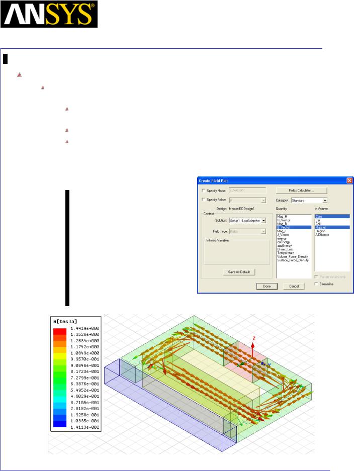
Maxwell v15 |
5.1 |
Example (Magnetostatic) – Magnetic Force
Plot Flux Density on Core Cross section
To ensure that the current direction and magnetization are correct, create a plot the flux density vector on the core cross section.
In the history tree, expand Planes and select the geometry on which to create the plot: Global:XY
Select the menu item Maxwell 3D > Fields > Fields > B > B_Vector
In Create Field plot window
1.Quantity: B_vector
2.In Volume: Press Ctrl and select Core and Magnet
3.Press Done
Note: This field plot is for the nominal design case with: mx = 1mm and c1 = 100A.
|
|
|
|
|
|
|
|
|
|
|
|
|
|
|
|
|
|
|
|
|
|
|
|
|
|
|
|
|
|
|
|
ANSYS Maxwell 3D Field Simulator v15 User’s Guide |
|
5.1-17 |
|||||
|
|
|
|
|
|
|
|

Maxwell v15 |
5.1 |
Example (Magnetostatic) – Magnetic Force
Optimetrics Setup – Parametric Sweep
During the design of a device, it is common practice to develop design trends based on swept parameters. Ansoft Maxwell 3D with Optimetrics Parametric Sweep can automatically create these design curves.
Add a Parametric Sweep
Select the menu item Maxwell 3D > Optimetrics Analysis > Add Parametric
In Setup Sweep Analysis window,
1.On the Sweep Definitions tab:
1.Click the Add button
2.Add/Edit Sweep Dialog
1.Select Variable: c1 (pull down menu to to change from “mx” if necessary)
2.Select Linear Step
3.Start: 0
4.Stop: 500
5.Step: 100
6.Click the Add button
7.Click the OK button
2.Click the Options tab:
1.Save Fields And Mesh: Checked
3.Click the OK button
Analyze Parametric Sweep
To start the solution process:
1.Expand the Project Tree to display the items listed under Optimetrics
2.Right-click the mouse on ParametricSetup1 and choose Analyze
|
|
|
|
|
|
|
|
|
|
|
|
|
|
|
|
|
|
|
|
|
|
|
|
|
|
|
|
|
|
|
|
ANSYS Maxwell 3D Field Simulator v15 User’s Guide |
|
5.1-18 |
|||||
|
|
|
|
|
|
|
|
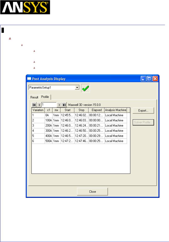
Maxwell v15 |
5.1 |
Example (Magnetostatic) – Magnetic Force
Optimetrics Results
To view the Optimetrics Results:
Select the menu item Maxwell 3D > Optimetrics Analysis > Optimetrics Results
Select the Profile Tab to view the solution progress for each setup. Click the Close button when you are finished viewing the results
|
|
|
|
|
|
|
|
|
|
|
|
|
|
|
|
|
|
|
|
|
|
|
|
|
|
|
|
|
|
|
|
ANSYS Maxwell 3D Field Simulator v15 User’s Guide |
|
5.1-19 |
|||||
|
|
|
|
|
|
|
|
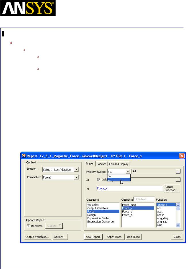
Maxwell v15 |
5.1 |
Example (Magnetostatic) – Magnetic Force
Create Plot of Force at each Current
To create a report:
Select the menu item Maxwell 3D> Results > Create Magnetostatic Report > Rectangular Plot
In Reports window
1.Solution: Setup1: LastAdaptive
2.Parameter: Force1
3.Click the Trace tab
1.Parametric Sweep : c1
2.X Axis: Default
3.Y Axis:
1.Category: Force
2.Quantity: Force_x
3.Function: <none>
4.Click the New Report button
|
|
|
|
|
|
|
|
|
|
|
|
ANSYS Maxwell 3D Field Simulator v15 User’s Guide |
|
5.1-20 |
|||
|
|
|
|
|
|
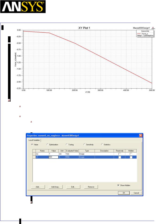
Maxwell v15 |
5.1 |
Example (Magnetostatic) – Magnetic Force
Plot Flux Density on Core Cross section at a different current
Finally, create a plot of B_vector in the core corresponding to the last row in the parametric table with c1 = 500A.
Switch to the solution for the last row in the parametric table:
Select Maxwell 3D > Design Properties > Local Variables. Change the value for c1 = 500 and click on OK.
The previous B_vector plot automatically updates to show the fields for c1 = 500A. The flux density is higher as expected
|
|
|
|
|
|
|
|
|
|
|
|
|
|
|
|
|
|
ANSYS Maxwell |
3D Field Simulator v15 User’s Guide |
|
|
5.1-21 |
||||
|
|
|
|
|
|
|
|
|
Maxwell v15 |
5.1 |
Example (Magnetostatic) – Magnetic Force
|
|
|
|
|
|
|
|
|
|
|
|
|
|
|
|
|
|
|
|
|
|
|
|
|
|
|
|
ANSYS Maxwell 3D Field Simulator v15 User’s Guide |
|
5.1-22 |
||||
|
|
|
|
|
|
|
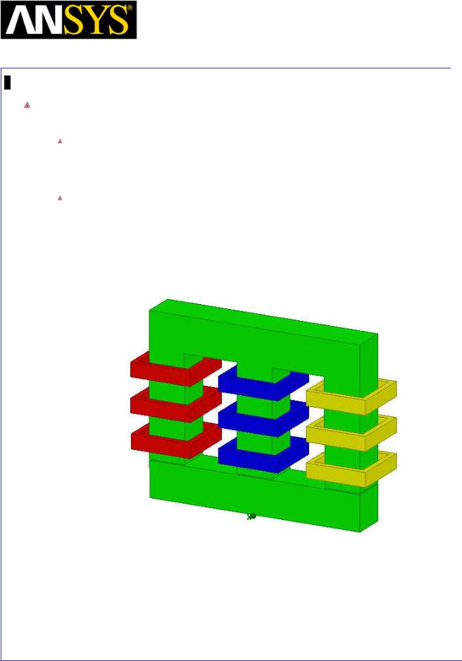
Maxwell v15 |
5.2 |
Example (Magnetostatic) – Inductance Calculation
The implementation and application of a 3-phase Inductor using the Magnetostatic Solver to calculate the nonlinear inductance
The inductance calculation is an important part of a magnetostatic simulation. The inductive properties will, of course, change with the nonlinearities of the problem. The properties and concepts of the inductance calculation are described in this example.
This example uses a 3-phase, 3-coil-per-phase inductor to demonstrate how the inductance calculation produces meaningful results. The setup is scrutinized and the results are examined. Then a half-symmetry model is examined to familiarize the user with a half-symmetry setup. Finally incremental inductance calculation was compared with apparent inductance in non-linear region of operation to define correct calculation.
|
|
|
|
|
|
|
|
|
|
|
|
ANSYS Maxwell 3D Field Simulator v15 User’s Guide |
|
5.2-1 |
|||
|
|
|
|
|
|
Maxwell v15 |
5.2 |
Example (Magnetostatic) – Inductance Calculation
ANSYS Maxwell Design Environment
The following features of the ANSYS Maxwell Design Environment are used to
create the models covered in this topic
3D Solid Modeling
Primitives: Box, Rectangle, Region
Surface Operations: Section
Boolean Operations: Subtract, Separate Bodies, Split
3D Modeler: Delete Last Operation
Sweep: Along Path
Duplicate: Along Line
Boundaries/Excitations
Current: Stranded
Analysis
Magnetostatic
Results
Inductance Matrix
|
|
|
|
|
|
|
|
|
|
|
|
|
|
|
|
|
|
|
|
|
|
|
|
|
|
|
|
|
|
|
|
ANSYS Maxwell 3D Field Simulator v15 User’s Guide |
|
5.2-2 |
|||||
|
|
|
|
|
|
|
|

Maxwell v15 |
5.2 |
Example (Magnetostatic) – Inductance Calculation
Launching Maxwell
To access Maxwell:
1.Click the Microsoft Start button, select Programs, and select Ansoft > Maxwell 15.0 and select Maxwell 15.0
Setting Tool Options
To set the tool options:
Note: In order to follow the steps outlined in this example, verify that the following tool options are set :
1. Select the menu item Tools > Options > Maxwell 3D Options
Maxwell Options Window:
1. Click the General Options tab
Use Wizards for data input when creating new boundaries: Checked
Duplicate boundaries/mesh operations with geometry:
Checked
2.Click the OK button
2.Select the menu item Tools > Options > Modeler Options.
Modeler Options Window:
1. Click the Operation tab
 Automatically cover closed polylines: Checked 2. Click the Display tab
 Default transparency = 0.8 3. Click the Drawing tab
 Edit property of new primitives: Checked 4. Click the OK button
|
|
|
|
|
|
|
|
|
|
|
|
|
|
|
|
|
|
|
|
|
|
|
|
|
|
|
|
|
|
|
|
ANSYS Maxwell 3D Field Simulator v15 User’s Guide |
|
5.2-3 |
|||||
|
|
|
|
|
|
|
|

Maxwell v15 |
5.2 |
Example (Magnetostatic) – Inductance Calculation
Opening a New Project
To open a new project:
After launching Maxwell, a project will be automatically created. You can also create a new project using below options.
1.In an Maxwell window, click the On the Standard toolbar, or select the menu item File > New.
Select the menu item Project > Insert Maxwell 3D Design, or click on the icon
Set Solution Type
To set the Solution Type:
Select the menu item Maxwell 3D > Solution Type
Solution Type Window:
1.Choose Magnetostatic
2.Click the OK button
|
|
|
|
|
|
|
|
|
|
|
|
|
|
|
|
|
|
|
|
|
|
|
|
|
|
|
|
|
|
|
|
ANSYS Maxwell 3D Field Simulator v15 User’s Guide |
|
5.2-4 |
|||||
|
|
|
|
|
|
|
|
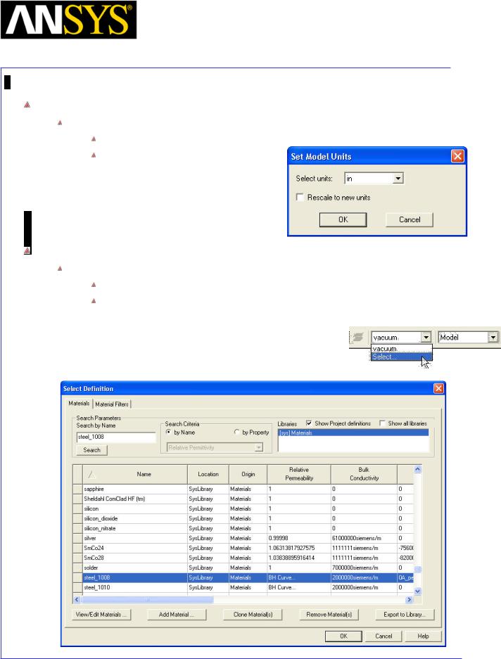
Maxwell v15 |
5.2 |
Example (Magnetostatic) – Inductance Calculation
Set Model Units
To Set the units:
Select the menu item Modeler > Units
Set Model Units:
1.Select Units: in (inches)
2.Click the OK button
Set Default Material
To set the default material:
Using the 3D Modeler Materials toolbar, choose Select
In Select Definition window,
1.Type steel_1008 in the Search by Name field
2.Click the OK button
|
|
|
|
|
|
|
|
|
|
|
|
|
|
|
|
|
|
|
|
|
|
|
|
|
|
|
|
|
|
|
|
ANSYS Maxwell 3D Field Simulator v15 User’s Guide |
|
5.2-5 |
|||||
|
|
|
|
|
|
|
|
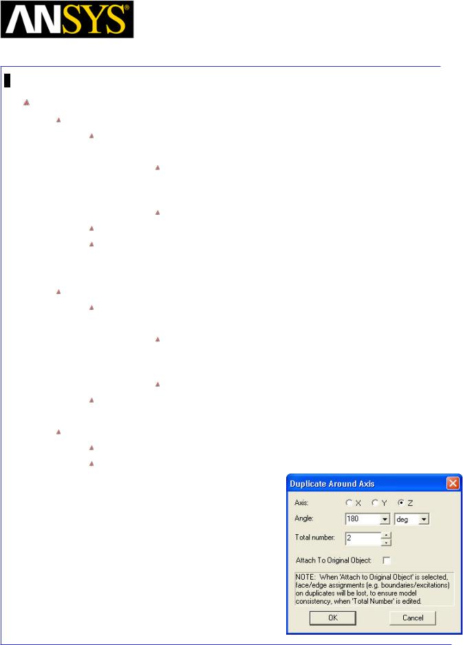
Maxwell v15 |
5.2 |
Example (Magnetostatic) – Inductance Calculation
Create Core
Create Box
Select the menu item Draw > Box
1. Using the coordinate entry fields, enter the box position X: -1, Y: -6, Z: 0, Press the Enter key
2.Using the coordinate entry fields, enter the opposite corner of the box:
dX: 2, dY: 12, dZ: 10, Press the Enter key
Select the menu item View > Fit All > Active View.
Select the resulting object from the tree and goto Properties window
1.Change the name of the object to Core
2.Change its color to Green
Create Another Box
Select the menu item Draw > Box
1. Using the coordinate entry fields, enter the box position X: -1, Y: 1, Z: 2, Press the Enter key
2.Using the coordinate entry fields, enter the opposite corner of the box:
dX: 2, dY: 3, dZ: 6, Press the Enter key
Select the resulting object from the tree and goto Properties window 1. Change the name of the object to Hole
Duplicate Hole
Select the object Hole from the history tree
Select the menu item Edit > Duplicate > Around Axis
1.Axis: Z
2.Angle: 180
3.Total Number: 2
4.Click the OK button
|
|
|
|
|
|
|
|
|
|
|
|
ANSYS Maxwell 3D Field Simulator v15 User’s Guide |
|
5.2-6 |
|||
|
|
|
|
|
|
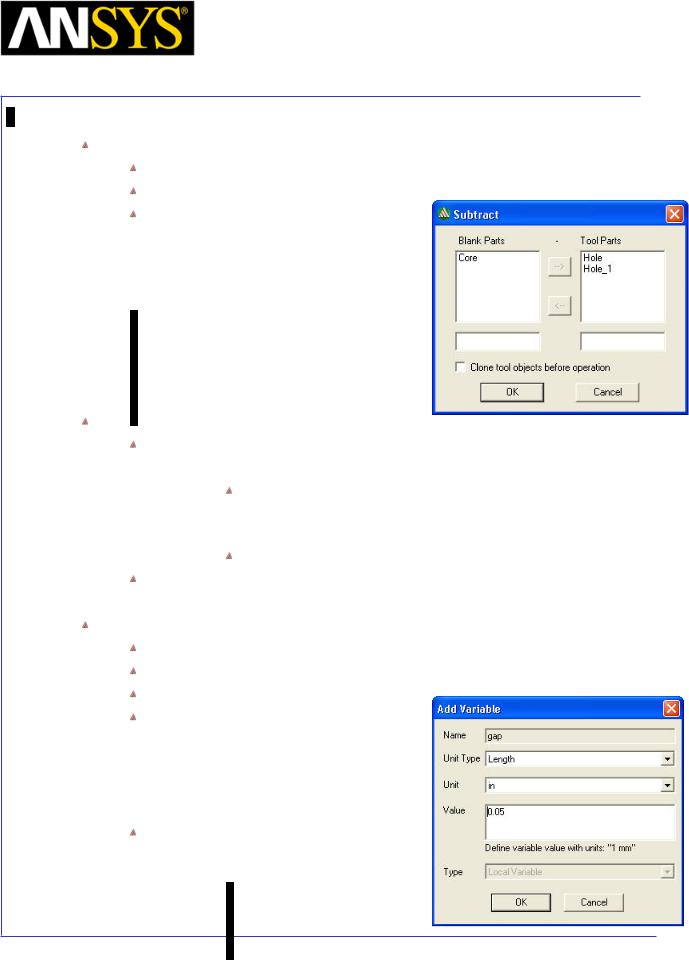
Maxwell v15 |
5.2 |
Example (Magnetostatic) – Inductance Calculation
Subtract Objects
Select the menu item Edit > Select All
Select the menu item, Modeler > Boolean > Subtract
In Subtract Window
1.Blank Parts: Core
2.Tool Parts: Hole and Hole_1
3.Click the OK button
Create Core_Gap
Select the menu item Draw > Box
1. Using the coordinate entry fields, enter the box position X: -1, Y: -6, Z: 2, Press the Enter key
2.Using the coordinate entry fields, enter the opposite corner of the box:
dX: 2, dY: 12, dZ: 0.05, Press the Enter key
Select the resulting object from the tree and goto Properties window 1. Change the name of the object to Core_Gap
Parameterize Gap
Expand the history tree of the object Core_Gap
Double click on the command CreateBox from the tree
For ZSize type: gap and press Enter In Add variable window,
1.Unit Type: Length
2.Unit: inch
3.Value: 0.05
4.Press OK
Press OK to exit
|
|
|
|
|
|
|
|
|
|
|
|
|
|
|
|
|
|
|
|
|
|
|
|
|
|
|
|
|
|
|
|
|
|
|
|
ANSYS Maxwell 3D Field Simulator v15 |
User’s Guide |
|
5.2-7 |
|||||
|
|
|
|
|
|
|
|
|
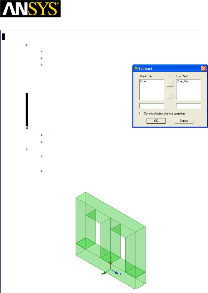
Maxwell v15 |
5.2 |
Example (Magnetostatic) – Inductance Calculation
Subtract Core
Press Ctrl and select the objects Core and Core_Gap from the history tree
Select the menu item Modeler > Boolean > Subtract
In Subtract Window,
1.Blank Parts: Core
2.Tool Parts: Core_Gap
3.Click the OK button
Separate Core
Select the object Core from the history tree
Select the menu item Modeler > Boolean > Separate Bodies
Change Attributes
Select the object Core from the tree and goto Properties window 1. Change the name of the object to Core_E
Select the object Core_Separate1 from the tree and goto Properties window
1. Change the name of the object to Core_I
|
|
|
|
|
|
|
|
|
|
|
|
|
|
|
|
|
|
|
|
|
|
|
|
|
|
|
|
|
|
|
|
ANSYS Maxwell 3D Field Simulator v15 User’s Guide |
|
5.2-8 |
|||||
|
|
|
|
|
|
|
|
Maxwell v15 |
5.2 |
Example (Magnetostatic) – Inductance Calculation
Set Default Material
To set the default material:
Using the 3D Modeler Materials toolbar, choose Select
In Select Definition window,
1.Type Copper in the Search by Name field
2.Click the OK button
Create Coils and Terminals
Create Rectangle
Select menu item Modeler > Grid Plane > YZ
Select menu item Draw > Rectangle.
1. Using the coordinate entry fields, enter the rectangle position X: 0, Y: -3.6, Z: 3.5, Press the Enter key
2.Using the coordinate entry fields, enter the opposite corner of the rectangle
dX: 0, dY: 0.3, dZ: -0.8, Press the Enter key
Select the resulting object from the tree and goto Properties window 1. Change the name of the object to CoilA_1
Create Guide
Select menu item Modeler > Grid Plane > XY
Select menu item Draw > Rectangle.
1. Using the coordinate entry fields, enter the rectangle position X: 1.5, Y: -6.5, Z: 3, Press the Enter key
2.Using the coordinate entry fields, enter the opposite corner of the rectangle
dX: -3, dY: 3, dZ: 0, Press the Enter key
Select the resulting object from the tree and goto Properties window 1. Change the name of the object to Guide
Select Guide from the tree and goto menu item Modeler > Delete Last Operation
Note: This operation will remove the cover closed polygon operation that is performed automatically. The results will be a rectangular polyline
|
|
|
|
|
|
|
|
|
|
|
|
|
|
ANSYS Maxwell |
3D Field Simulator v15 User’s Guide |
|
5.2-9 |
|||
|
|
|
|
|
|
|
Maxwell v15 |
5.2 |
Example (Magnetostatic) – Inductance Calculation
Sweep Object
Press Ctrl and select the objects CoilA_1 and Guide from the history tree
Select menu item Draw > Sweep > Along Path
In Sweep along path window
1.Angle of twist: 0 deg
2.Draft Angle: 0 deg
3.Draft type: Round
4.Select OK
Create Section for CoilA_1
Select the object CoilA_1 from the history tree
Select the menu item Modeler > Surface > Section
In Section window,
1.Section Plane: YZ
2.Click the OK button
Rename CoilA_1_Section1 to TerminalA_1
Separate Sheets
Select the sheet TerminalA_1 resulted in last operation
Select the menu item Modeler > Boolean > Separate Bodies
Delete the extra sheet TerminalA_1_Seperate1
|
|
|
|
|
|
|
|
|
|
|
|
|
|
|
|
|
|
|
|
|
|
|
|
|
|
|
|
|
|
|
|
ANSYS Maxwell 3D Field Simulator v15 User’s Guide |
|
5.2-10 |
|||||
|
|
|
|
|
|
|
|
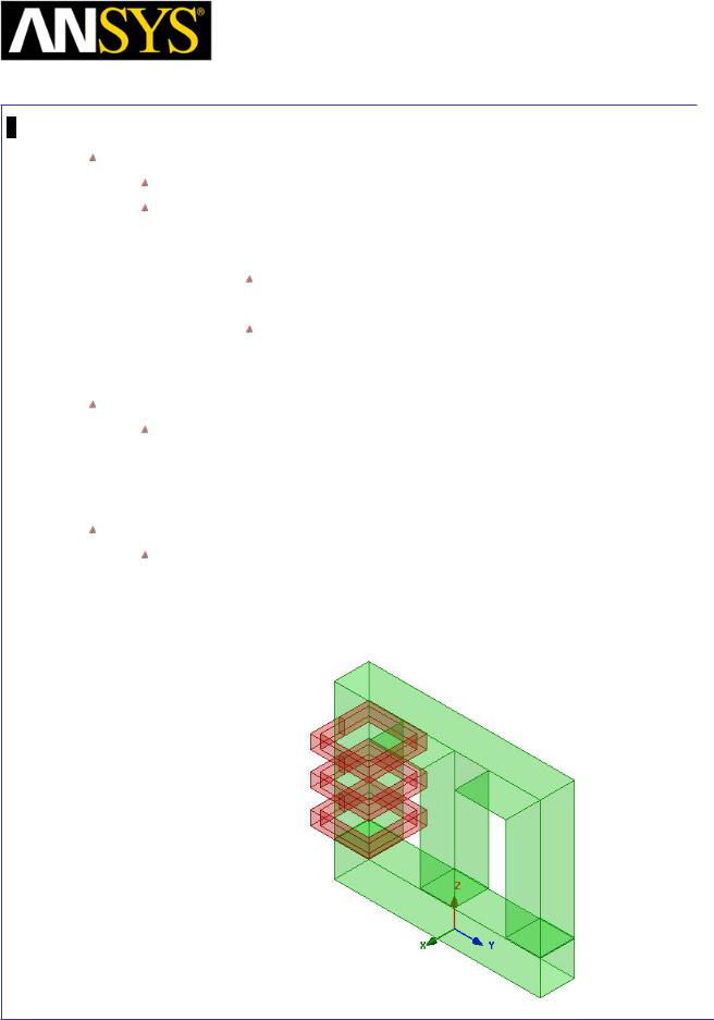
Maxwell v15 |
5.2 |
Example (Magnetostatic) – Inductance Calculation
Duplicate Objects
Press Ctrl and select the objects CoilA_1 and TerminalA_1 from the tree Select menu item Edit > Duplicate > Along Line
1.Using the coordinate entry fields, enter the first point of duplicate vector
X: 0, Y: 0, Z: 0, Press the Enter key
2. Using the coordinate entry fields, enter the second point dX: 0, dY: 0, dZ: 1.925, Press the Enter key
3.Total Number : 3
4.Press OK
Change Attributes of Coils
Select the resulting objects from the tree and goto Properties window
1.Change the name of the object CoilA_1_1 to CoilA_2
2.Change the name of the object CoilA_1_2 to CoilA_3
3.Change color of CoilA_1,CoilA_2 and CoilA_3 to Red
Change Attributes of Terminals
Select the resulting objects from the tree and goto Properties window
1.Change the name of the object TerminalA_1_1 to TerminalA_2
2.Change the name of the object TerminalA_1_2 to TerminalA_3
3.Change color of TerminalA_1,TerminalA_2 and TerminalA_3 to Red
|
|
|
|
|
|
|
|
|
|
|
|
|
|
|
|
|
|
|
|
|
|
|
|
|
|
|
|
|
|
|
|
ANSYS Maxwell 3D Field Simulator v15 User’s Guide |
|
5.2-11 |
|||||
|
|
|
|
|
|
|
|
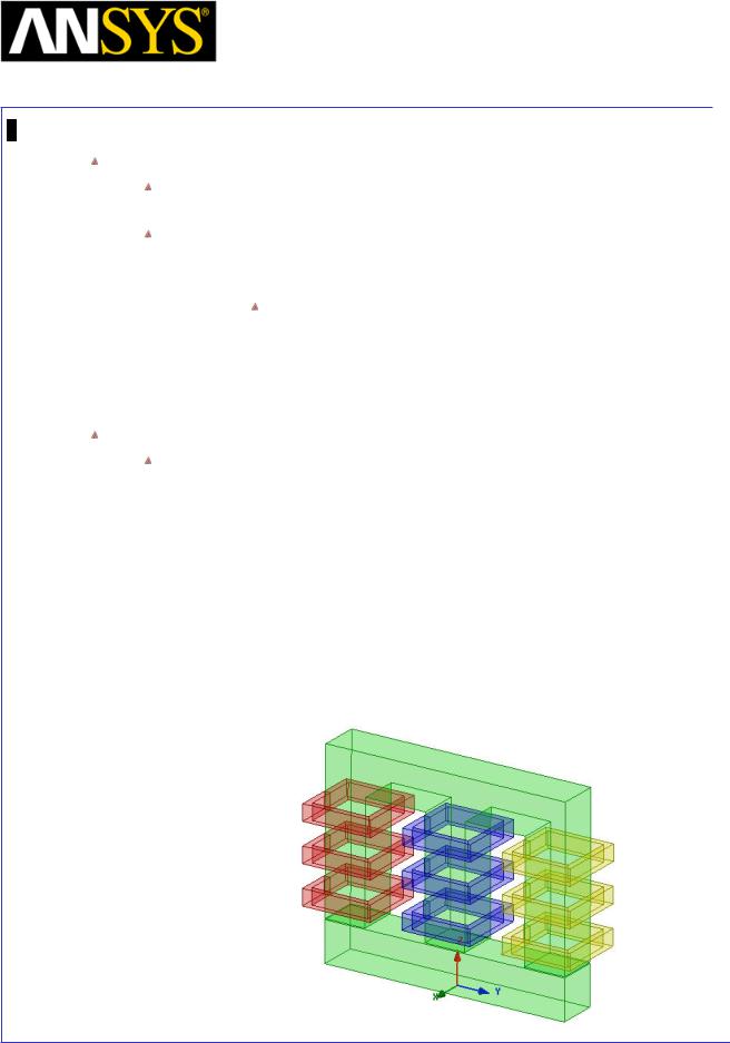
Maxwell v15 |
5.2 |
Example (Magnetostatic) – Inductance Calculation
Duplicate Coils
Press Ctrl and select the object CoilA_1, CoilA_2 ,CoilA_3,TerminalA_1, TerminalA_2 and TerminalA_3 from the tree
Select menu item Edit > Duplicate > Along Line
1.Using the coordinate entry fields, enter the first point of duplicate vector
X: 0, Y: 0, Z: 0, Press the Enter key
2. Using the coordinate entry fields, enter the second point
3.
4.
 dX: 0, dY: 5, dZ: 0, Press the Enter key Total Number : 3
Press OK
Change Attributes
Select the resulting objects from the tree and goto Properties window
1.Change the name of the objects CoilA_1_1, CoilA_2_1 and CoilA_3_1 to CoilB_1, CoilB_2 and CoilB_3
2.Change the name of the objects CoilA_1_2, CoilA_2_2 and CoilA_3_2 to CoilC_1, CoilC_2 and CoilC_3
3.Change the name of the terminals TerminalA_1_1, TerminalA_2_1, TerminalA_3_1, TerminalA_1_2, TerminalA_2_2 and TerminalA_3_2 to TerminalB_1, TerminalB_2, TerminalB_3, TerminalC_1, TerminalC_2 and TerminalC_3
4.
5.
Change color of all CoilB and TerminalB objects to Blue Change color of all CoilC and TerminalC objects to Yellow
|
|
|
|
|
|
|
|
|
|
|
|
|
|
|
|
|
|
|
|
|
|
|
|
|
|
|
|
|
|
|
|
ANSYS Maxwell 3D Field Simulator v15 User’s Guide |
|
5.2-12 |
|||||
|
|
|
|
|
|
|
|
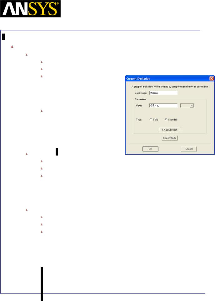
Maxwell v15 |
5.2 |
Example (Magnetostatic) – Inductance Calculation
Create Excitations
Assign Excitation to TerminalA
Press Ctrl and select objects TerminalA_1, TerminalA_2 and TerminalA_3
Select the menu item Maxwell 3D > Excitations > Assign > Current
In Current Excitation window,
1.Name: PhaseA
2.Value: -0.5*Mag
3.Type: Stranded
4.Press OK
In Add variable window,
1.Unit Type: Current
2.Unit: A
3.Value: 30
4.Press OK
Assign Excitation to TerminalB
Press Ctrl and select objects TerminalB_1, TerminalB_2 and TerminalB_3
Select the menu item Maxwell 3D > Excitations > Assign > Current
In Current Excitation window,
1.Name: PhaseB
2.Value: Mag
3.Type: Stranded
4.Press OK
Assign Excitation to TerminalC
Press Ctrl and select objects TerminalC_1, TerminalC_2 and TerminalC_3
Select the menu item Maxwell 3D > Excitations > Assign > Current
In Current Excitation window,
1.Name: PhaseC
2.Value: -0.5*Mag
3.Type: Stranded
4.Press OK
|
|
|
|
|
|
|
|
|
|
|
|
|
|
|
|
|
|
ANSYS Maxwell 3D Field Simulator v15 User’s Guide |
|
5.2-13 |
|||
|
|
|
|
|
|
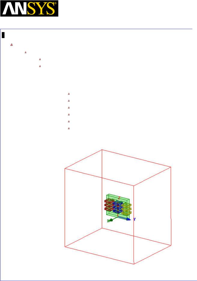
Maxwell v15 |
5.2 |
Example (Magnetostatic) – Inductance Calculation
Define Region
Create Simulation Region
Select the menu item Draw > Region
In Region window,
1.Padding Data: Pad individual directions
2.Padding Type: Percentage Offset
3.Directions:
+X = 400
-X = 400
+Y = 100
-Y = 100
+Z = 150 -Z = 150
Press OK
|
|
|
|
|
|
|
|
|
|
|
|
|
|
|
|
|
|
|
|
|
|
|
|
|
|
|
|
|
|
|
|
ANSYS Maxwell 3D Field Simulator v15 User’s Guide |
|
5.2-14 |
|||||
|
|
|
|
|
|
|
|

Maxwell v15 |
5.2 |
Example (Magnetostatic) – Inductance Calculation
Inductance Calculation Defining Equations
Inductance in a magnetostatic simulation can be defined as
λ1 = L11I1 + L12 I2 +
λ2 = L21I1 + L22 I2 +
where λ is the flux linkage for an individual coil, and I is the current.
This inductance is the apparent inductance – it defines the ratio of flux linkage to current in one coil.
The inductance of a coil can also be defined by the energy storage as
L = 2×W I 2
I 2
= ∫B HdΩ I 2
where the energy is determined by the magnetic flux density and field intensity in the solution space.
This energy storage calculation is what determines the inductance values in the matrix. The on-diagonal elements (L11, L22, etc.) are determined by exciting the coils individually and finding the energy from the B and H fields for each individual case. The off-diagonal elements (L12, L21, L13, etc.) are determined from a combination of the B and H fields from the individually excited cases. The following is the exact defining equation for the inductance calculation
Lij = ∫Bi H j dΩ
where it is assumed that one ampere is flowing through the respective coils.
For nonlinear materials, the value of the inductance obtained from these calculations is only valid for the specific source currents. If any of the source currents change, the characteristics of the field solution will change as well as the inductance of each coil (less change when in a linear region, greatest change when moving from the linear region to a saturated region).
If only linear materials are used, the value of the inductance will be valid for any value of source currents.
|
|
|
|
|
|
|
|
|
|
|
|
ANSYS Maxwell 3D Field Simulator v15 User’s Guide |
|
5.2-15 |
|||
|
|
|
|
|
|
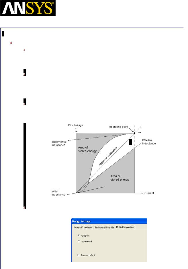
Maxwell v15 |
5.2 |
Example (Magnetostatic) – Inductance Calculation
Inductance Calculation Methodology
The inductance calculation is performed after the field solution and depends on the values of the field solution at every point in the solution space because it requires an energy integral in the entire solution space.
After the field solution is completed, the relative permeability values are “frozen”. Then, one ampere is sequentially excited in each coil, and a field solution is performed with the frozen permeabilities. With these field solutions, the energy integral is performed and the inductance is obtained as described previously.
The inductance obtained in this manner is the inductance per turn^2 (referred to as the nominal inductance in the software) and is the apparent inductance (determined by the flux linkage/current operating point in the graphic below).
Incremental inductance can also be obtained using Maxwell by setting the parameter Maxwell 3D > Design Settings > Matrix Computation to the value Incremental
|
|
|
|
|
|
|
|
|
|
|
|
ANSYS Maxwell 3D Field Simulator v15 User’s Guide |
|
5.2-16 |
|||
|
|
|
|
|
|
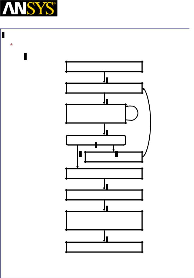
Maxwell v15 |
5.2 |
Example (Magnetostatic) – Inductance Calculation
Inductance Calculation Process
Initial Setup
Adaptive Solution
Nonlinear Convergence (Changing permeability)
Solution Convergence ?
Refine Mesh
Converged or Number of Passes
Permeability is Frozen
Inductance Matrix Solution
(Linear solution process)
Matrix Post Processing
|
|
|
|
|
|
|
|
|
|
|
|
ANSYS Maxwell 3D Field Simulator v15 User’s Guide |
|
5.2-17 |
|||
|
|
|
|
|
|

Maxwell v15 |
5.2 |
Example (Magnetostatic) – Inductance Calculation
Inductance Calculation Post Processing
The nominal inductances that are computed by the solver are returned in units of Henries/turns^2. In order to return each inductance in units of Henries, the number of turns for each coil must be specified at some point. Also, the inductance matrix can be grouped to represent windings in series, and a factor can be included if the winding is made up of parallel branches. These are all considered post-processing, and they can help to return meaningful quantities.
The post processed inductances are calculated as follows:
Lij = Ni N j Lij _ nom
Lgroup = ∑ ∑Lij
i _ group j _ group
Lbranched = Lgroup  b2
b2
The first step is to find the coil inductances from the nominal inductances by multiplying by the number of turns in each coil (or number of turns squared for self inductances).
The next step is to group the series inductances by adding up all the inductances in the block (i.e. if conductors 1 through N are grouped, then add up the N by N block of inductances to obtain the grouped self inductance – the same process is followed for grouped mutual inductances).
The final step is to take into account parallel branches by dividing by the number of branches squared. The inductance decreases with parallel branches because of the reduced number of turns per branch.
|
|
|
|
|
|
|
|
|
|
|
|
ANSYS Maxwell 3D Field Simulator v15 User’s Guide |
|
5.2-18 |
|||
|
|
|
|
|
|
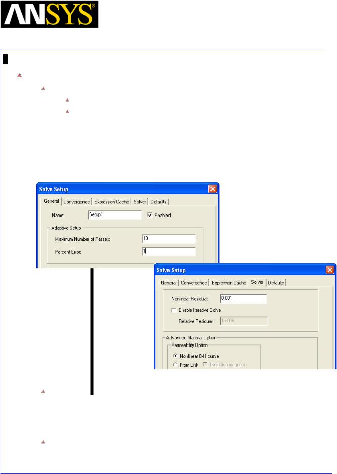
Maxwell v15 |
5.2 |
Example (Magnetostatic) – Inductance Calculation
Analysis Setup
To create an analysis setup:
Select the menu item Maxwell 3D > Analysis Setup > Add Solution Setup
Solution Setup Window:
1. General Tab
 Percentage Error: 1 2. Solver Tab
 Nonlinear Residuals : 0.001 3. Click the OK button
The Nonlinear Residual is important in simulations with nonlinear materials that operate outside of the linear region. Increasing the number will make the simulation run faster, decreasing the number will force the nonlinear solver to more precisely find the nonlinear B-H operating points within the steel (or other nonlinear magnetic material).
It is often the case with saturated nonlinear materials that the Nonlinear Residual will need to be reduced to obtain accurate results.
|
|
|
|
|
|
|
|
|
|
|
|
|
|
|
|
|
|
|
|
|
|
|
|
|
|
|
|
5.2-19 |
|||
ANSYS Maxwell 3D Field Simulator v15 User’s Guide |
|
|
|||||
|
|
|
|
|
|
|
|
Maxwell v15 |
5.2 |
Example (Magnetostatic) – Inductance Calculation
Create Matrix Parameters
Create parameters for 30 Turns of Coil
Select the menu item Maxwell 3D > Parameters > Assign > Matrix
In Matrix window, 1. Solver Tab:
Include : Checked for all sources
2.In Post Processing Tab
1.Turns : Specify 30 for each of the sources
2.Press Ctrl and select PhaseA_1, PhaseA_2 and PhaseA_3
3.Select Group
4.Rename the group created as PhaseA
5.Leave Branches to 1
6.In similar way, create groups PhaseB and PhaseC
3.Press OK
This setup says that each source has 30 turns and that the sources on each leg are connected in series (as far as the post-processing is concerned).
|
|
|
|
|
|
ANSYS Maxwell 3D Field Simulator v15 User’s Guide |
5.2-20 |
||||
|
|
|
|
|
|
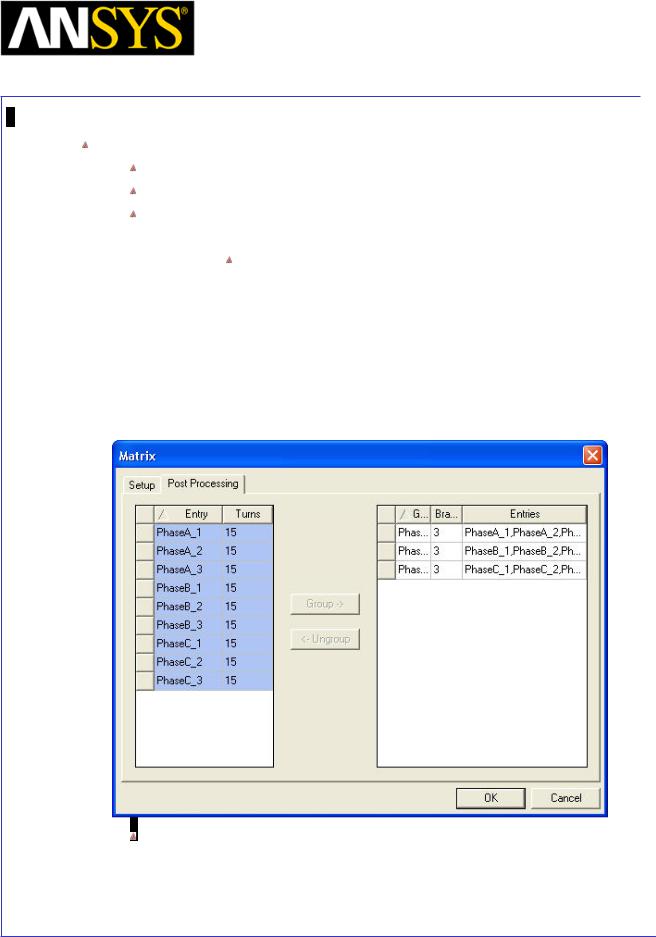
Maxwell v15 |
5.2 |
Example (Magnetostatic) – Inductance Calculation
Create parameters for 15 Turns of Coil
We will create a second Matrix Parameter to show what the settings signify.
Select the menu item Maxwell 3D > Parameters > Assign > Matrix
In Matrix window, 1. Solver Tab:
Include : Checked for all sources
2.In Post Processing Tab
1.Turns : Specify 15 for each of the sources
2.Press Ctrl and select PhaseA_1, PhaseA_2 and PhaseA_3
3.Select Group
4.Rename the group created as PhaseA
5.Change Branches to 3
6.In similar way, create groups PhaseB and PhaseC
This setup says that each source has 15 turns in 3 branches of 15 turns each (with twice the current in each turn as for the 30 turn case) and that the sources on each leg are connected in series (as far as the postprocessing is concerned).
|
|
|
|
|
|
|
|
|
|
|
|
|
|
|
|
|
|
|
|
|
|
|
|
|
|
|
|
5.2-21 |
|||
ANSYS Maxwell 3D Field Simulator v15 User’s Guide |
|
|
|||||
|
|
|
|
|
|
|
|
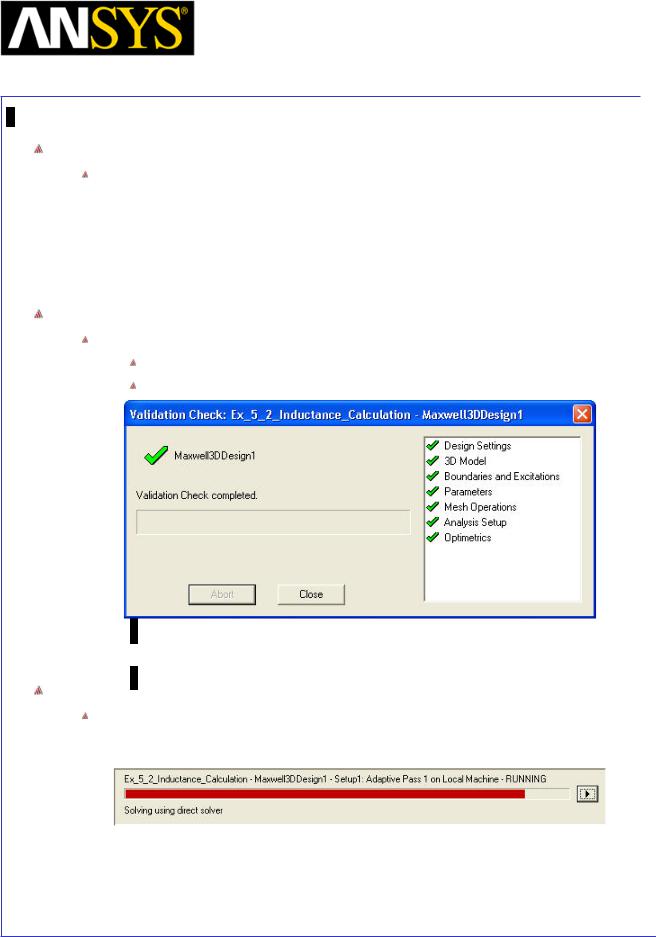
Maxwell v15 |
5.2 |
Example (Magnetostatic) – Inductance Calculation
Save Project
To save the project:
1.In an Ansoft Maxwell window, select the menu item File > Save As.
2.From the Save As window, type the Filename: Ex_5_2_Inductance_Calculation
3.Click the Save button
Model Validation
To validate the model:
Select the menu item Maxwell 3D > Validation Check
Click the Close button
Note: To view any errors or warning messages, use the Message Manager.
Analyze
To start the solution process:
1. Select the menu item Maxwell 3D > Analyze All
|
|
|
|
|
|
|
|
|
|
|
|
|
|
|
|
|
|
|
|
|
|
|
|
|
|
|
|
|
|
|
|
ANSYS Maxwell 3D Field Simulator v15 User’s Guide |
|
5.2-22 |
|||||
|
|
|
|
|
|
|
|
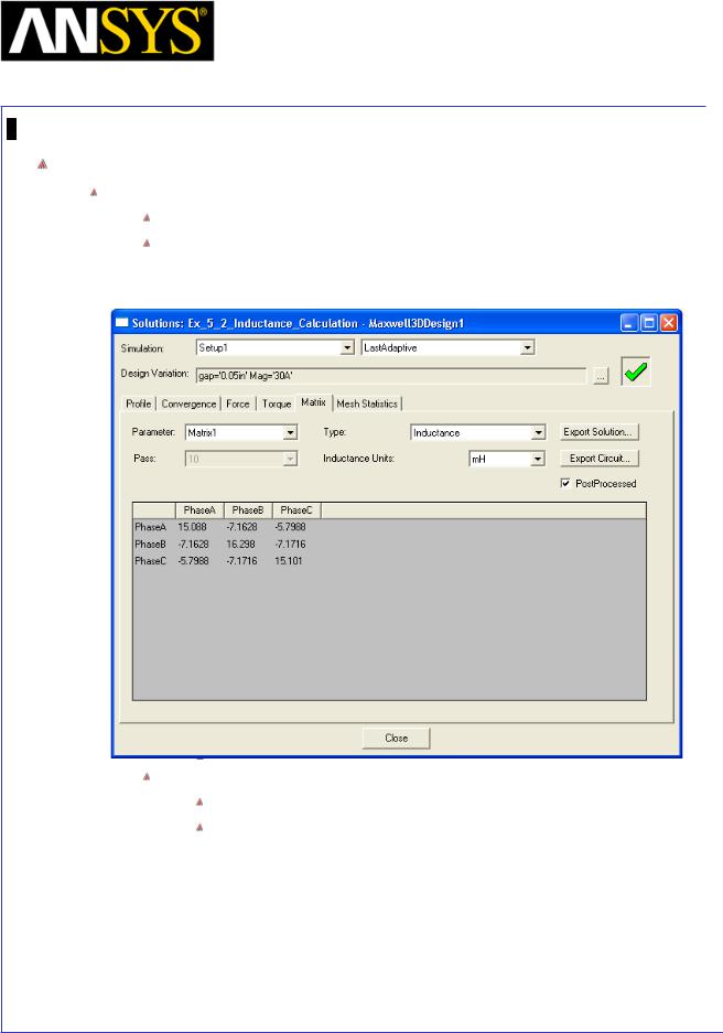
Maxwell v15 |
5.2 |
Example (Magnetostatic) – Inductance Calculation
Solution Data
To view the Solution Data:
Select the menu item Maxwell 3D > Results > Solution Data
Matrix Tab
1.By default, non-postprocessed data is shown for Matrix1
2.Change the option PostProcessed: Checked
Note:
Results are symmetric in both axes as we would expect.
Mutual inductances are negative. It is important to note that the direction of the current used for the mutual inductances is determined by the direction of the arrow for each excitation
|
|
|
|
|
|
|
|
|
|
|
|
|
|
|
|
|
|
|
|
|
|
|
|
|
|
|
|
|
|
|
|
ANSYS Maxwell 3D Field Simulator v15 User’s Guide |
|
5.2-23 |
|||||
|
|
|
|
|
|
|
|
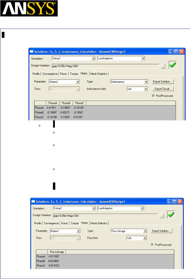
Maxwell v15 |
5.2 |
Example (Magnetostatic) – Inductance Calculation
3. Change Parameter to Matrix2
Note:
Notice that the results change to reflect twice the turns and one-third the branches (2^2 * 3^2 = 36 times the previous inductance value).
Remember that by increasing the turns, the current in each turn is decreased to keep the total ampere-turns constant – this is very important for nonlinear materials. The solutions apply only for this value of current.
If you were to compare the non-post processed results for both matrices, you would see that these values are the same.
4.Change Parameter to Matrix1 and the Solution Type to Flux Linkage to see either the Post Processed or nominal flux linkage values.
|
|
|
|
|
|
|
|
|
|
|
|
|
|
|
|
|
|
|
|
|
|
|
|
|
|
|
|
|
|
|
|
|
|
|
|
|
|
|
|
|
|
|
|
|
|
|
|
|
|
ANSYS Maxwell 3D Field Simulator v15 User’s Guide |
|
5.2-24 |
|||||||
|
|
|
|
|
|
|
|
|
|

Maxwell v15 |
5.2 |
Example (Magnetostatic) – Inductance Calculation
Results and Interpretations
These results are being obtained from a magnetostatic simulation with arbitrary constant current inputs defined for each leg. The notation used was in terms of 3 phases, which might imply that this is an AC inductor of some sort. The modeling of AC currents in a magnetostatic simulation can sometimes be valid for instantaneous values (of force and inductance), but the requirements are that eddy currents do not effect the solution (either a low frequency source or low loss materials). The other two options available in the Maxwell software are eddy current simulations (which allows AC sources, but does not allow nonlinear materials), and transient simulations (which allows the study of nonlinear and AC phenomena).
This type of magnetostatic simulation would also be valuable for an Equivalent Circuit Extraction (again, eddy currents should be negligible) - this would require each phase to be excited as a variable, and run as a full parametric simulation including all phases across all possible current values (at least 5^3 variations to see any nonlinear behavior). Notice that if you do an equivalent circuit extraction of the inductance, the flux values automatically take into account the grouping and other post-processing values specified in the matrix parameter.
Other magnetostatic results can be obtained from this simulation, such as force on the Core_I object and magnetic field in the steel (is it saturating?).
Remember that this simulation uses nonlinear materials, so all of the solutions are only valid for this specific set of excitations. If you were to change the input currents, then you will have to solve again to see how the inductance and other results change.
Another important note is that although we included 2 matrix parameters, this is not necessary to see differently post-processed results. You can edit the postprocessing characteristics of the matrix after having solved the problem, and the results will adjust to reflect the changes without needing to resolve. The only time that you would need multiple matrices is if one matrix or the other did not include all the coils. By using two matrices, the inductance calculation was performed twice, lengthening the simulation. The point of this example was to show that multiple matrix parameters can be defined – not to suggest using multiple matrix parameters.
|
|
|
|
|
|
|
|
|
|
|
|
|
|
|
|
|
|
|
|
|
|
|
|
|
|
|
|
5.2-25 |
|||
ANSYS Maxwell 3D Field Simulator v15 User’s Guide |
|
|
|||||
|
|
|
|
|
|
|
|
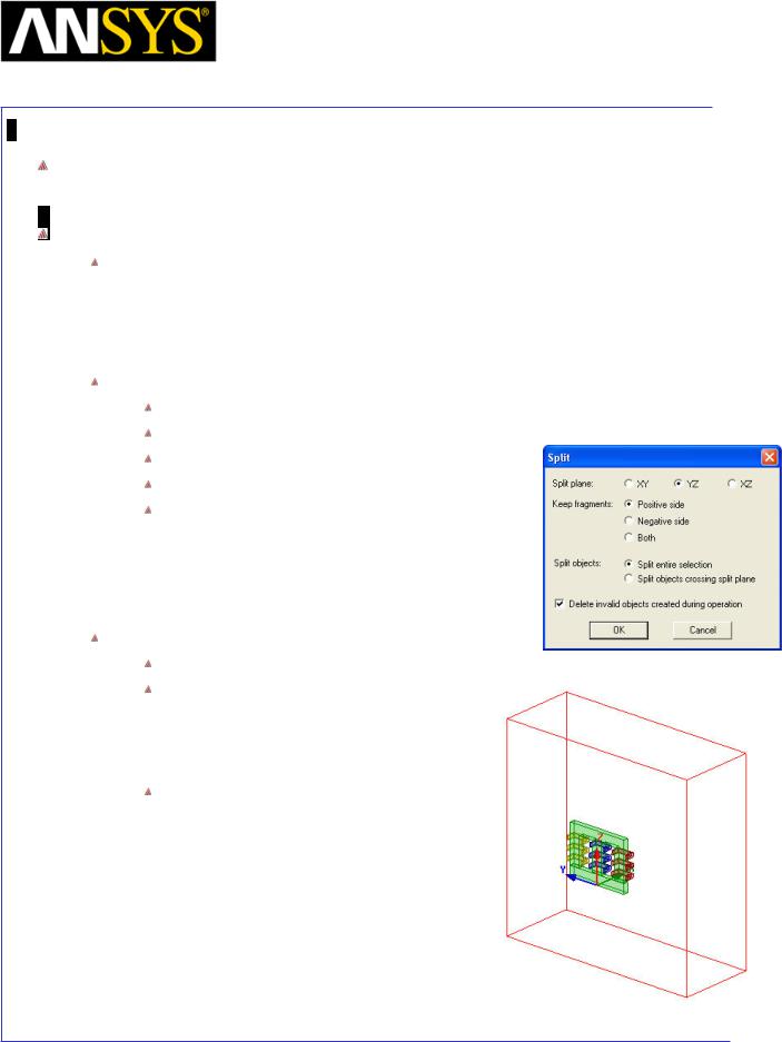
Maxwell v15 |
5.2 |
Example (Magnetostatic) – Inductance Calculation
Example 2: Solving Symmetry Model
Create Symmetry Design
Copy Design
1.Select Maxwell3D Design1 in Project Manager window, right click and select Copy
2.Select project Ex_5_2_Inductance_Calculation in Project Manager window and select Paste
Split Geometry
Select Region from the history tree
Select the menu item View > Visibility> Hide Selection > Active View
Select the menu item Edit > Select All Visible
Select menu item Modeler > Boolean > Split
In Split window
1.Split plane: YZ
2.Keep fragments: Positive side
3.Split objects: Split entire selection
4.Press OK
Modify Region
Select menu item Draw > Region
In Properties window,
1.+X Padding Data: 800
2.-X padding Data: 0
3.Press OK
Select menu item View > Visibility >
Show All > Active View to view Region
|
|
|
|
|
|
|
|
|
|
|
|
|
|
|
|
|
|
|
|
|
|
|
|
|
|
|
|
|
|
|
|
ANSYS Maxwell 3D Field Simulator v15 User’s Guide |
|
5.2-26 |
|||||
|
|
|
|
|
|
|
|
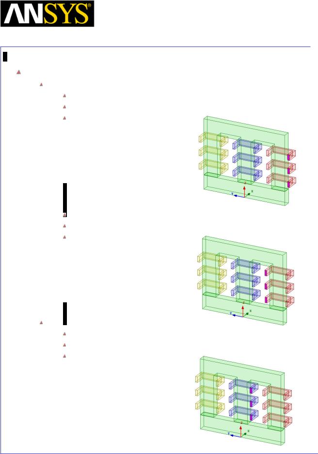
Maxwell v15 |
5.2 |
Example (Magnetostatic) – Inductance Calculation
Specify Excitations
Create Excitation for CoilA
Press Ctrl and select faces of CoilA as shown in image
Select menu item Maxwell 3D > Excitations > Assign > Current
In Current Excitation window,
1.Name: PhaseA_in
2.Value: -0.5*Mag
3.Type: Stranded
4.Direction: Positive X
5.Press OK
Press Ctrl and select faces of CoilA as shown in below image
Select menu item Maxwell 3D > Excitations > Assign > Current
In Current Excitation window,
1.Name: PhaseA_out
2.Value: -0.5*Mag
3.Type: Stranded
4.Direction: Negative X
5.Press OK
Create Excitations for CoilB
Press Ctrl and select faces of CoilB as shown in below image
Select menu item Maxwell 3D > Excitations > Assign > Current
In Current Excitation window,
1.Name: PhaseB_in
2.Value: Mag
3.Type: Stranded
4.Direction: Positive X
5.Press OK
|
|
|
|
|
|
|
|
|
|
|
|
|
|
|
|
|
|
|
|
|
|
|
|
|
|
|
|
|
|
|
|
ANSYS Maxwell 3D Field Simulator v15 User’s Guide |
|
5.2-27 |
|||||
|
|
|
|
|
|
|
|
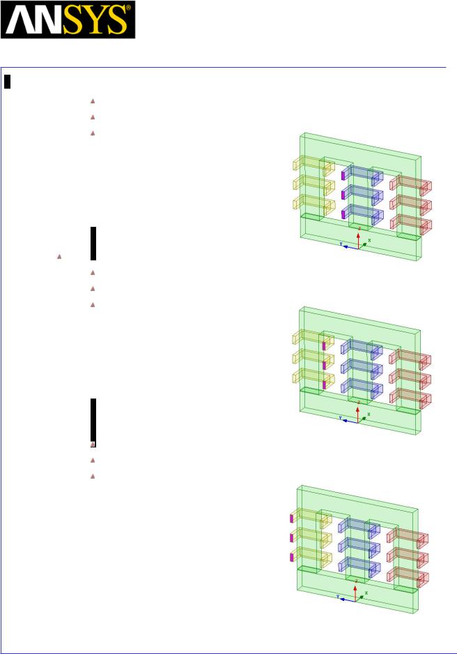
Maxwell v15 |
5.2 |
Example (Magnetostatic) – Inductance Calculation
Press Ctrl and select faces of CoilA as shown in below image
Select menu item Maxwell 3D > Excitations > Assign > Current
In Current Excitation window,
1.Name: PhaseB_out
2.Value: Mag
3.Type: Stranded
4.Direction: Negative X
5.Press OK
Create Excitation for CoilC
Press Ctrl and select faces of CoilC as shown in below image
Select menu item Maxwell 3D > Excitations > Assign > Current
In Current Excitation window,
1.Name: PhaseC_in
2.Value: -0.5*Mag
3.Type: Stranded
4.Direction: Positive X
5.Press OK
Press Ctrl and select faces of CoilC as shown in below image
Select menu item Maxwell 3D > Excitations > Assign > Current
In Current Excitation window,
1.Name: PhaseC_out
2.Value: -0.5*Mag
3.Type: Stranded
4.Direction: Negative X
5.Press OK
|
|
|
|
|
|
|
|
|
|
|
|
|
|
|
|
|
|
|
|
|
|
|
|
|
|
|
|
|
|
|
|
|
|
|
|
|
|
|
|
|
|
|
|
|
|
|
|
|
|
ANSYS Maxwell 3D Field Simulator v15 User’s Guide |
|
5.2-28 |
|||||||
|
|
|
|
|
|
|
|
|
|
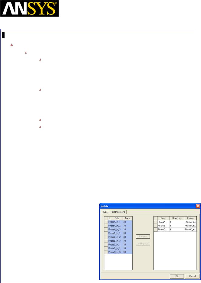
Maxwell v15 |
5.2 |
Example (Magnetostatic) – Inductance Calculation
Create Matrix Parameters
Note:
When matrix parameters are defined, a check will be performed for proper conduction paths and for terminals correctly defined across a cross-section of the conduction paths. Several errors can appear when defining a matrix, and these often have to do with the definition of the conducting objects or the excitation.
The excitations that appear in the matrix setup, are those excitations that are pointing into the conductor. So, for a symmetry model that requires two excitations per conductor, only one excitation per conductor will be listed in the matrix setup – this excitation will be the one pointing into the modeled conductor.
Select the menu item Maxwell 3D > Parameters > Assign > Matrix
In Matrix window, 1. Solver Tab:
 Include : Checked for all sources 2. In Post Processing Tab
1.
2.
Turns : Specify 30 for each of the sources
Press Ctrl and select PhaseA_in_1, PhaseA_in_2 and PhaseA_in_3
3.
4.
5.
6.
Select Group
Rename the group created as PhaseA Leave Branches to 1
In similar way, create groups PhaseB and PhaseC
3. Press OK
|
|
|
|
|
|
|
|
|
|
|
|
|
|
|
|
|
|
|
|
|
|
|
|
|
|
|
|
|
|
|
|
ANSYS Maxwell 3D Field Simulator v15 User’s Guide |
|
5.2-29 |
|||||
|
|
|
|
|
|
|
|
Maxwell v15 |
5.2 |
Example (Magnetostatic) – Inductance Calculation
Model Validation
To validate the model:
Select the menu item Maxwell 3D > Validation Check
Click the Close button
Note: To view any errors or warning messages, use the Message Manager.
Analyze
To start the solution process:
1. Select the menu item Maxwell 3D > Analyze All
|
|
|
|
|
|
|
|
|
|
|
|
ANSYS Maxwell 3D Field Simulator v15 User’s Guide |
|
5.2-30 |
|||
|
|
|
|
|
|
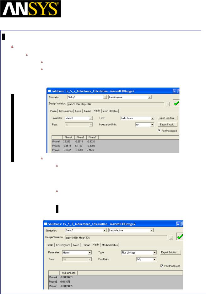
Maxwell v15 |
5.2 |
Example (Magnetostatic) – Inductance Calculation
Solution Data
To view the Solution Data:
Select the menu item Maxwell 3D > Results > Solution Data
Matrix Tab
1.By default, non-postprocessed data is shown for Matrix1
2.Change the option PostProcessed: Checked
Note:
Notice that the results are half the value that we obtained for the full model. This is very important to remember when using these values. The halved results are consistent for other parameters and properties as well (i.e. torque, total energy, etc.)
If these values are used to create an Equivalent Circuit Extraction, remember to use a scaling factor of 2 to account for the symmetry.
3.Change the Solution Type to Flux Linkage to see either the Post Processed or nominal flux linkage values.
|
|
|
|
|
|
|
|
|
|
|
|
|
|
|
|
|
|
|
|
|
|
|
|
|
|
|
|
|
|
|
|
ANSYS Maxwell 3D Field Simulator v15 User’s Guide |
|
5.2-31 |
|||||
|
|
|
|
|
|
|
|
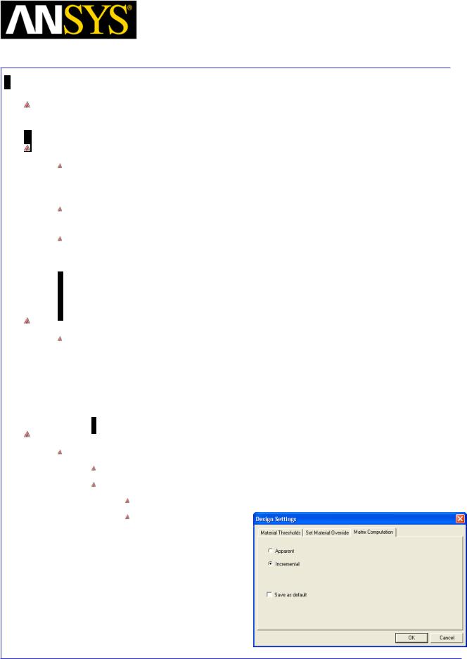
Maxwell v15 |
5.2 |
Example (Magnetostatic) – Inductance Calculation
Example 2: Incremental Inductance Calculation
Incremental Inductance Calculation
Apparent inductance calculation works fine when material operation is within the linear region of BH Curve. When material is operating in non-linear region, inductance calculation with apparent method may not correct.
In Such cases Incremental inductance gives better results compared to apparent inductance.
Incremental inductance value is calculated using slope of the Flux linkage vs Current graph at material operating point.
Ldjk = |
∂λj |
∂ik |
Create Symmetry Design
Copy Design
1.Select Maxwell3D Design1 in Project Manager window, right click and select Copy
2.Select project Ex_5_2_Inductance_Calculation in Project Manager window and select Paste
Change Inductance Calculation Method
To Change inductance Calculation method
Select the menu item Maxwell 3D > Design Settings
In Design Settings window,
Select the tab Matrix Computation
Press OK
|
|
|
|
|
|
|
|
|
|
|
|
|
|
|
|
|
|
|
|
|
|
|
|
|
|
|
|
|
|
|
|
|
|
|
|
|
|
|
|
|
|
|
|
|
|
|
|
|
|
|
|
|
|
|
|
|
|
|
|
ANSYS Maxwell 3D Field Simulator v15 User’s Guide |
|
5.2-32 |
|||||||
|
|
|
|
|
|
|
|
|
|
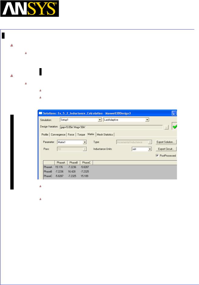
Maxwell v15 |
5.2 |
Example (Magnetostatic) – Inductance Calculation
Analyze
To start the solution process:
1. Select the menu item Maxwell 3D > Analyze All
Solution Data
To view the Solution Data:
Select the menu item Maxwell 3D > Results > Solution Data
Matrix Tab
1. PostProcessed: Checked
It can be seen that the results are almost the same as well got with apparent inductance calculation method.
Now we will drive the core into nonlinear region of operation and check the impact
|
|
|
|
|
|
|
|
|
|
|
|
|
|
|
|
|
|
|
|
|
|
|
|
|
|
|
|
|
|
|
|
ANSYS Maxwell 3D Field Simulator v15 User’s Guide |
|
5.2-33 |
|||||
|
|
|
|
|
|
|
|
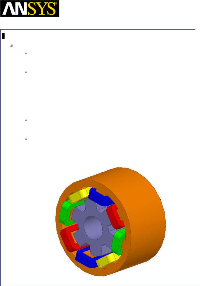
Maxwell v15 |
5.3 |
Example (Magnetostatic) – Stranded Conductors
Stranded Conductors
This example is intended to show you how to create and analyze a magnetostatic problem with stranded conductors for a Switched Reluctance Motor geometry using Magnetostatic solver in the ANSYS Maxwell 3D Design Environment.
Within the Maxwell 3D Design Environment, complete coils can be modeled as Stranded Conductors. There are many advantages to using Stranded Conductors when modeling coils that have multiple turns. The first obvious advantage is that a coil with multiple wires, say 2500, can be modeled as a single object as opposed to modeling each wire which would be impracticable. Secondly, defining a Stranded Conductor means that the current density will be uniform throughout the cross section of the conductor which is physically correct for a coil with many turns.
The example that will be used to demonstrate how Stranded Conductors are implemented in a switched Reluctance Motor. This switched reluctance motor will have four phases and two coils per phase.
Note: There is no fundamental difference between how stranded conductors are treated in the Eddy Current solver as compared to the Magnetostatic Solver. When using the Eddy Current Solver and specifying Stranded for the terminal excitation the Eddy Effect is automatically turned off
|
|
|
|
|
|
|
|
|
|
|
|
ANSYS Maxwell 3D Field Simulator v15 User’s Guide |
|
5.3-1 |
|||
|
|
|
|
|
|
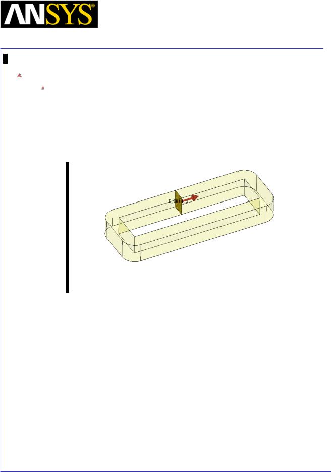
Maxwell v15 |
5.3 |
Example (Magnetostatic) – Stranded Conductors
Theory – Magnetostatic Solver
When using the Magnetostatic Solver, with a Stranded Current Source, the solver assumes the following conditions:
1.The current density is uniformly distributed over the cross section of the terminal as well as through the entire conductor.
2.The direction of the current is indicated by the arrow as seen on the terminal. Change the direction of the current by clicking on Swap Direction in the Current Excitation window to reverse the flow.
3.The solver does not know how many turns are represented by the coil, thus the value of current that is being applied represents the total ampere-turns. For this example, the value 3570 could represent any of the following:
1.1 amp thru 3570 turns
2.5 amps thru 750 turns
3.25 amps thru 150 turns
4.3570 amps thru 1 turn
or any such combination that produces a value of 3750 ampere-turns. The ratio of amperes to turns does not impact the field solution or the value of inductance reported in the inductance matrix. However, this value of inductance assumes a 1 turn coil, and must be multiplied by N2 to determine the actual inductance of the coil. Please refer to the overview for details of the inductance calculation.
|
|
|
|
|
|
|
|
|
|
|
|
ANSYS Maxwell 3D Field Simulator v15 User’s Guide |
|
5.3-2 |
|||
|
|
|
|
|
|

Maxwell v15 |
5.3 |
Example (Magnetostatic) – Stranded Conductors
Theory – Magnetostatic Solver (Continued)
The ampere-turn value used to define the current source is used to calculate the current density which is the initial condition used by the solver according to the
equation:
I
J = S n
Where: I is the total current in ampere-turns
S is the area of the terminal in m2
nis the unit normal direction
J is the Current Density vector in A/m2
The path of the current is determined by the conduction path. Select the menu item Maxwell > Excitations > Conduction Paths to view the conduction path, and verify that the conduction path is correct. In this example, if any of the coils touched the stator, then this would constitute a separate conduction path since the material properties of the stator has a conductivity value 2e6 siemens/meter; to solve this problem an insulation boundary will need to be applied to the coils or stator; please refer to the overview section for details on insulation boundaries.
Although the Magnetostatic solver uses the current density vector J as the initial condition, it does not solve for J directly as part of the output solution matrix. The quantity that the Magnetostatic solver directly calculates is the magnetic field intensity H. From H, the current density J in any conductor is derived by:
J = × H
|
|
|
|
|
|
|
|
|
|
|
|
ANSYS Maxwell 3D Field Simulator v15 User’s Guide |
|
5.3-3 |
|||
|
|
|
|
|
|

Maxwell v15 |
5.3 |
Example (Magnetostatic) – Stranded Conductors
ANSYS Maxwell Design Environment
The following features of the ANSYS Maxwell Design Environment are used to
create the models covered in this topic
3D Solid Modeling
User Defined Primitives (UDP): Switched Reluctance Motor
Primitives: Regular Polyhedron
Surface Operations: Section
Boolean Operations: Separate Bodies
Boundaries/Excitations
Current: Stranded
Analysis
Magnetostatic
Results
Field Calculator
Field Overlays:
Magnitude B
|
|
|
|
|
|
|
|
|
|
|
|
|
|
|
|
|
|
|
|
|
|
|
|
|
|
|
|
|
|
|
|
ANSYS Maxwell 3D Field Simulator v15 User’s Guide |
|
5.3-4 |
|||||
|
|
|
|
|
|
|
|

Maxwell v15 |
5.3 |
Example (Magnetostatic) – Stranded Conductors
Launching Maxwell
To access Maxwell:
1.Click the Microsoft Start button, select Programs, and select Ansoft > Maxwell 15.0 and select Maxwell 15.0
Setting Tool Options
To set the tool options:
Note: In order to follow the steps outlined in this example, verify that the following tool options are set :
1. Select the menu item Tools > Options > Maxwell 3D Options
Maxwell Options Window:
1. Click the General Options tab
Use Wizards for data input when creating new boundaries: Checked
Duplicate boundaries/mesh operations with geometry:
Checked
2.Click the OK button
2.Select the menu item Tools > Options > Modeler Options.
Modeler Options Window:
1. Click the Operation tab
 Automatically cover closed polylines: Checked 2. Click the Display tab
 Default transparency = 0.8 3. Click the Drawing tab
 Edit property of new primitives: Checked 4. Click the OK button
|
|
|
|
|
|
|
|
|
|
|
|
|
|
|
|
|
|
|
|
|
|
|
|
|
|
|
|
|
|
|
|
ANSYS Maxwell 3D Field Simulator v15 User’s Guide |
|
5.3-5 |
|||||
|
|
|
|
|
|
|
|

Maxwell v15 |
5.3 |
Example (Magnetostatic) – Stranded Conductors
Opening a New Project
To open a new project:
After launching Maxwell, a project will be automatically created. You can also create a new project using below options.
1.In an Maxwell window, click the On the Standard toolbar, or select the menu item File > New.
Select the menu item Project > Insert Maxwell 3D Design, or click on the icon
Set Solution Type
To set the Solution Type:
Select the menu item Maxwell 3D > Solution Type
Solution Type Window:
1.Choose Magnetostatic
2.Click the OK button
|
|
|
|
|
|
|
|
|
|
|
|
|
|
|
|
|
|
|
|
|
|
|
|
|
|
|
|
|
|
|
|
ANSYS Maxwell 3D Field Simulator v15 User’s Guide |
|
5.3-6 |
|||||
|
|
|
|
|
|
|
|
Maxwell v15 |
5.3 |
Example (Magnetostatic) – Stranded Conductors
Set Model Units
To Set the units:
Select the menu item Modeler > Units
Set Model Units:
1.Select Units: mm
2.Click the OK button
Set Default Material
To set the default material:
Using the 3D Modeler Materials toolbar, choose Select
In Select Definition window,
1.Type steel_1008 in the Search by Name field
2.Click the OK button
|
|
|
|
|
|
|
|
|
|
|
|
|
|
|
|
|
|
|
|
|
|
|
|
|
|
|
|
|
|
|
|
ANSYS Maxwell 3D Field Simulator v15 User’s Guide |
|
5.3-7 |
|||||
|
|
|
|
|
|
|
|
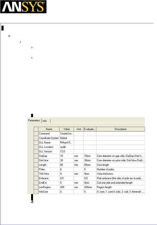
Maxwell v15 |
5.3 |
Example (Magnetostatic) – Stranded Conductors
Create Rotor
To Create Rotor
Select the menu item Draw > User Defined Primitive > SysLib > RMxprt > SRMCore
In User Defined Primitive Operation window
1.For the value of DiaGap, type: 70, Click the Tab key to accept
2.For the value of DiaYoke, type: 30, Click the Tab key to accept
3.For the value of Length, type: 65, Click the Tab key to accept
4.For the value of Poles, type: 6, Click the Tab key to accept
5.For the value of ThkYoke, type: 9, Click the Tab key to accept
6.For the value of Embrace, type: 0.5, Click the Tab key to accept
7.For the value of EndExt, type: 0, Click the Tab key to accept
8.For the value of InfoCore, type: 0, Click the Tab key to accept
9.Click the OK button
Select the menu item View > Fit All > Active View.
|
|
|
|
|
|
|
|
|
|
|
|
|
|
|
|
|
|
|
|
|
|
|
|
ANSYS Maxwell 3D Field Simulator v15 User’s Guide |
|
5.3-8 |
|||||
|
|
|
|
|
|
|
|
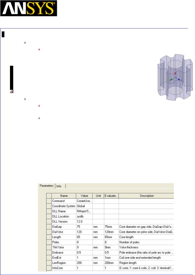
Maxwell v15 |
5.3 |
Example (Magnetostatic) – Stranded Conductors
Change Attributes
Select the resulting object from the tree and goto Properties window 1. Change the name of the object to Rotor
Create Stator and Coil
To Create Stator and Coils
Select the menu item Draw > User Defined Primitive > SysLib > RMxprt > SRMCore
In User Defined Primitive Operation window
1.For the value of DiaGap, type: 75, Click the Tab key to accept
2.For the value of DiaYoke, type: 120, Click the Tab key to accept
3.For the value of Length, type: 65, Click the Tab key to accept
4.For the value of Poles, type: 8, Click the Tab key to accept
5.For the value of ThkYoke, type: 9, Click the Tab key to accept
6.For the value of Embrace, type: 0.5, Click the Tab key to accept
7.For the value of EndExt, type: 1, Click the Tab key to accept
8.For the value of InfoCore, type: 1, Click the Tab key to accept
9.Click the OK button
|
|
|
|
|
|
|
|
|
|
|
|
|
|
|
|
|
|
|
|
|
|
|
|
|
|
|
|
|
|
|
|
|
|
|
|
|
|
|
|
|
|
|
|
|
|
|
|
|
|
|
|
|
|
|
|
|
|
|
|
ANSYS Maxwell 3D Field Simulator v15 User’s Guide |
|
5.3-9 |
|||||||
|
|
|
|
|
|
|
|
|
|
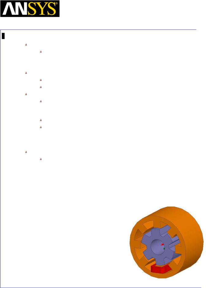
Maxwell v15 |
5.3 |
Example (Magnetostatic) – Stranded Conductors
Change Attributes
Select the resulting object from the tree and goto Properties window
1.Change the name of the object to Stator
2.Change its color to Orange
Separate Coils
Select the object Stator from the tree
Select the menu item Modeler > Boolean > Separate Bodies
Delete Unwanted Objects
Select the objects Stator_Separate2, Stator_Separate3, Stator_Separate4, Stator_Separate5, Stator_Separate6, Stator_Separate7 and Stator_Separate8 from the tree
Select the menu item Edit > Delete
Note: We have kept only one coil and deleted others. We will recreate other coils after excitations are specified for one coil. This way we can copy coil terminal and excitation from one coil to all other coils. Thus we will can save time needed to specify excitation for each coil.
Change Attributes
Select the object Stator_Separate1 from the tree and goto Properties window
1.Change the name of the object to Coil_A1
2.Change its color to Red
3.Goto Material tab and select Edit
4.In Select Definition window,
1.Type copper in the Search by Name field
2.Click the OK button
|
|
|
|
|
|
|
|
|
|
|
|
|
|
|
|
|
|
|
|
|
|
|
|
|
|
|
|
|
|
|
|
|
|
|
|
|
|
|
|
|
|
|
|
|
|
|
|
|
|
|
|
|
|
|
|
|
|
|
|
|
|
|
|
|
|
|
|
|
|
|
|
|
|
|
|
|
|
|
|
|
|
|
|
ANSYS Maxwell 3D Field Simulator v15 User’s Guide |
|
5.3-10 |
|||||||||
|
|
|
|
|
|
|
|
|
|
|
|
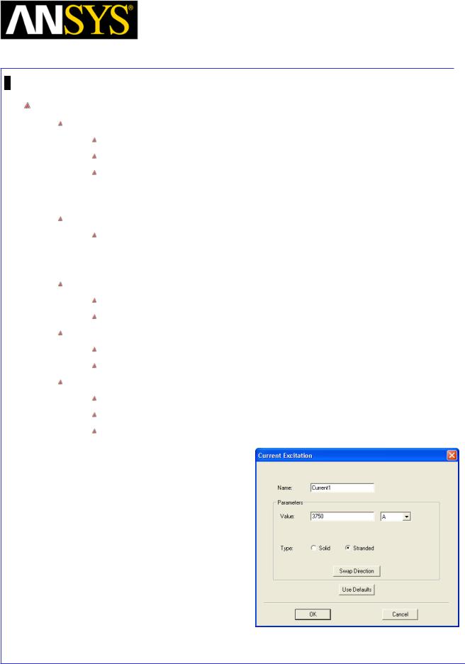
Maxwell v15 |
5.3 |
Example (Magnetostatic) – Stranded Conductors
Create Excitations
Create Section
Select the object Coil_A1 from the tree
Select the menu item Modeler > Surface >Section
In Section window,
1.Section Plane: XY
2.Click the OK button
Change Attributes
Select the object Coil_Section1 from the tree and goto Properties window
1.Change the name of the object to Terminal_A1
2.Change its color to Red
Separate Sections
Select the object Terminal_A1 from the tree
Select the menu item Modeler > Boolean > Separate Bodies
Delete Extra Sheets
Select the object Terminal_A1_Separate1 from the tree
Select the menu item Edit > Delete
Assign Excitation
Select the object Terminal_A1
Select the menu item Maxwell 3D > Excitations > Assign >Current
In Current Excitation window,
1.Name: Current1
2.Value: 3750 A
3.Type: Stranded
4.Press OK
|
|
|
|
|
|
|
|
|
|
|
|
|
|
|
|
|
|
|
|
|
|
|
|
|
|
|
|
|
|
|
|
|
|
|
|
|
|
|
|
|
|
|
|
|
|
|
|
|
|
|
|
|
|
|
|
|
|
|
|
|
|
|
|
|
|
|
|
|
|
|
|
|
|
|
|
|
|
|
|
|
|
|
|
|
|
|
|
|
|
|
|
|
|
|
|
ANSYS Maxwell 3D Field Simulator v15 User’s Guide |
|
5.3-11 |
|||||||||
|
|
|
|
|
|
|
|
|
|
|
|
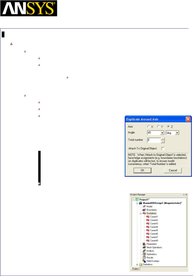
Maxwell v15 |
5.3 |
Example (Magnetostatic) – Stranded Conductors
Duplicate Coil with Excitations
Verify Duplicate Boundary Option is Set
Select the menu item Tools > Options > Maxwell 3D Options
Maxwell Options Window:
1. Click the General Options tab
Duplicate boundaries/mesh operations with geometry: Checked
2. Click the OK button Duplicate Objects
Select the object Coil_A1 and sheet Terminal_A1 from the tree
Select the menu item Edit > Duplicate > Around Axis
In Duplicate Around Axis window,
1.Axis: Z
2.Angle: 45deg
3.Total Number: 8
4.Click the OK button
Note: As we have copies Terminals with the above option set, excitations are also copied for each terminal. In the tree now total eight excitations can be seen.
|
|
|
|
|
|
|
|
|
|
|
|
|
|
|
|
|
|
|
|
|
|
|
|
|
|
|
|
|
|
|
|
ANSYS Maxwell 3D Field Simulator v15 User’s Guide |
|
5.3-12 |
|||||
|
|
|
|
|
|
|
|
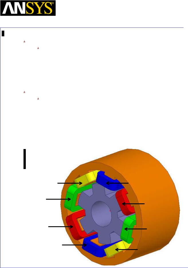
Maxwell v15 |
5.3 |
Example (Magnetostatic) – Stranded Conductors
Change Attributes for Coils
Select the resulting object from the tree and goto Properties window
1.Change the name of the objects Coil_A1_1, Coil_A1_2, Coil_A1_3, Coil_A1_4, Coil_A1_5, Coil_A1_6 and Coil_A1_7 to Coil_B1, Coil_C1, Coil_D1, Coil_A2, Coil_B2, Coil_C2 and Coil_D2
2.
3.
4.
Change the color of the objects Coil_B1 and Coil_B2 to Blue Change the color of the objects Coil_C1 and Coil_C2 to Yellow Change the color of the objects Coil_D1 and Coil_D2 to Green
Change Attributes for Terminals
Select the resulting object from the tree and goto Properties window
1.Change the name of the sheets Terminal_A1_1, Terminal_A1_2, Terminal_A1_3, Terminal_A1_4, Terminal_A1_5, Terminal_A1_6 and Terminal_A1_7 to Terminal_B1, Terminal_C1, Terminal_D1, Terminal_A2, Terminal_B2, Terminal_C2 and Terminal_D2
2.
3.
4.
Change color of the sheets Terminal_B1 and Terminal_B2 to Blue Change color of the sheets Terminal_C1 and Terminal_C2 to Yellow Change color of the sheets Terminal_D1 and Terminal_D2 to Green
Coil_C2 |
Coil_B2 |
Coil_D2 |
Coil_A2 |
|
Coil_A1 |
Coil_D1 |
|
Coil_B1
Coil_C1
|
|
|
|
|
|
|
|
|
|
|
|
ANSYS Maxwell 3D Field Simulator v15 User’s Guide |
|
5.3-13 |
|||
|
|
|
|
|
|
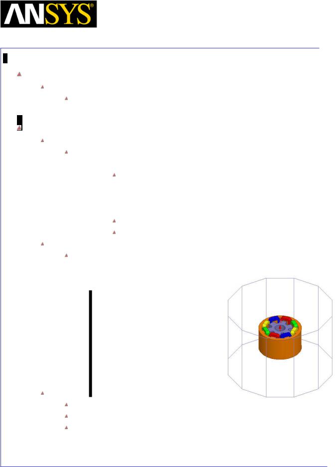
Maxwell v15 |
5.3 |
Example (Magnetostatic) – Stranded Conductors
Set Default Material
To Set Default Material
Using the 3D Modeler Materials toolbar, choose Vacuum
Create Region
To create the region:
Select the menu item Draw > Regular Polyhedron
1. Using the coordinate entry fields, enter the center position
X: 0.0, Y: 0.0, Z: -100.0, Press the Enter key
2. Using the coordinate entry fields, enter the radius and height:
 dX: 150.0 dY: 0.0, dZ: 200.0, Press the Enter key 3. Segment Number Window
Number of Segments: 12
Click the OK button
Change Attributes
Select the resulting object from the tree and goto Properties window
1.Change the name of the object to Region
2.Display Wireframe: Checked
Hide Region
Select Region from the history tree
Select the menu item View >Visibility > Hide Selection > Active View
Select the menu item View > Fit All > Active View.
|
|
|
|
|
|
|
|
|
|
|
|
|
|
|
|
|
|
|
|
|
|
|
|
ANSYS Maxwell 3D Field Simulator v15 User’s Guide |
|
5.3-14 |
|||||
|
|
|
|
|
|
|
|
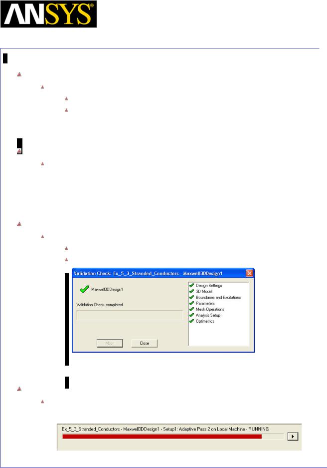
Maxwell v15 |
5.3 |
Example (Magnetostatic) – Stranded Conductors
Analysis Setup
To create an analysis setup:
Select the menu item Maxwell 3D > Analysis Setup > Add Solution Setup
Solution Setup Window:
1. Click the OK button to accept all default settings.
Save Project
To save the project:
1.In an Ansoft Maxwell window, select the menu item File > Save As.
2.From Save As window, type the Filename: Ex_5_3_Stranded_Conductors
3.Click the Save button
Model Validation
To validate the model:
Select the menu item Maxwell 3D > Validation Check
Click the Close button
Note: To view any errors or warning messages, use the Message Manager.
Analyze
To start the solution process:
1. Select the menu item Maxwell 3D > Analyze All
|
|
|
|
|
|
|
|
|
|
|
|
ANSYS Maxwell 3D Field Simulator v15 User’s Guide |
|
5.3-15 |
|||
|
|
|
|
|
|
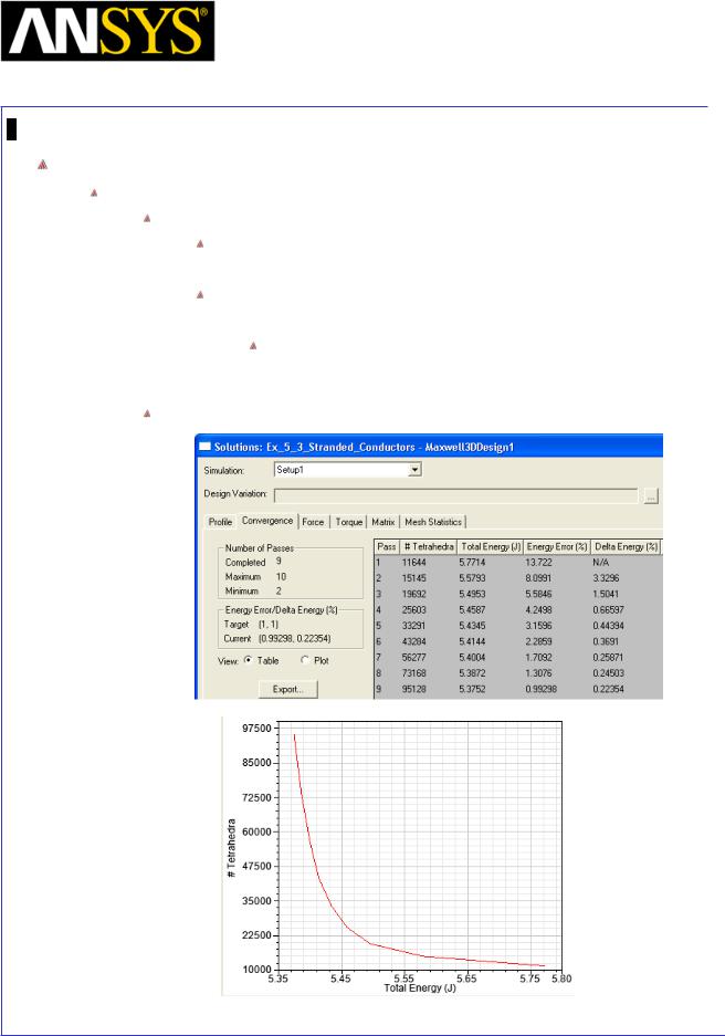
Maxwell v15 |
5.3 |
Example (Magnetostatic) – Stranded Conductors
Solution Data
To view the Solution Data:
Select the menu item Maxwell 3D > Results > Solution Data
To view the Profile:
1. Click the Profile Tab. To view the Convergence:
1. Click the Convergence Tab
Note: The default view is for convergence is Table. Select the Plot radio button to view a graphical representations of the convergence data.
Click the Close button
|
|
|
|
|
|
|
|
|
|
|
|
|
|
|
|
|
|
|
|
|
|
|
|
|
|
|
|
|
|
|
|
ANSYS Maxwell 3D Field Simulator v15 User’s Guide |
|
5.3-16 |
|||||
|
|
|
|
|
|
|
|
Maxwell v15 |
5.3 |
Example (Magnetostatic) – Stranded Conductors
Create Field Overlay
To create a field plot:
Select the objects Stator and Rotor from the tree
Select the menu item Maxwell 3D > Fields > Fields > B > Mag_B
In the Create Field Plot window:
1.Solution: Setup1 : LastAdaptive
2.Quantity: Mag_B
3.Plot on Surface Only: Checked
4.Click the Done button
|
|
|
|
|
|
|
|
|
|
|
|
|
|
|
|
|
|
|
|
|
|
|
|
|
|
|
|
|
|
|
|
|
|
|
|
|
|
|
|
|
|
|
|
|
|
|
|
|
|
|
|
|
|
|
|
|
|
|
|
ANSYS Maxwell 3D Field Simulator v15 User’s Guide |
|
5.3-17 |
|||||||
|
|
|
|
|
|
|
|
|
|
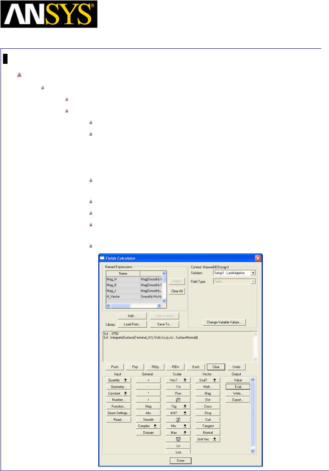
Maxwell v15 |
5.3 |
Example (Magnetostatic) – Stranded Conductors
Calculate Current
Use the field calculator to verify the total amp-turns flowing in the winding:
Select the menu item Maxwell 3D > Fields > Calculator
In Fields Calculator window,
Select Input > Quantity > J
Select Input > Geometry
1.Select the radio button Surface
2.From the list select: Terminal_A1
3.Click the OK button
Select Vector > Normal to determine the current normal to the terminal
Select ∫ (Integrate)
Click the Eval button to evaluate the results
Note: Value reported by calculator is current in Ampere-Turns flowing through the coil which is equal to 3750
Press Done to exit calculator
|
|
|
|
|
|
|
|
|
|
|
|
|
|
|
|
|
|
|
|
|
|
|
|
|
|
|
|
|
|
|
|
ANSYS Maxwell 3D Field Simulator v15 User’s Guide |
|
5.3-18 |
|||||
|
|
|
|
|
|
|
|
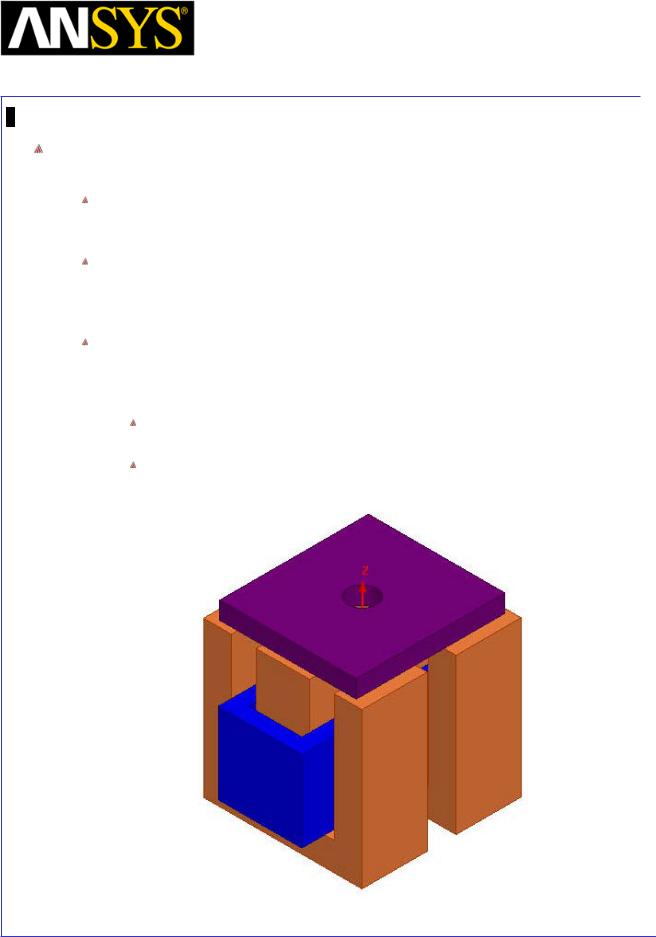
Maxwell v15 |
5.4 |
Example (Magnetostatic) – ECE: Linear Movement
Realization of an equivalent circuit extraction (ECE) of a problem with linear movement
The Electro Mechanical software package provided by ANSYS enables system simulation as well as component simulation. Often, the results of an in depth study of a magnetic component are needed in a top level, system analysis.
With Maxwell, the results of a parametric analysis can be used to generated an Equivalent Circuit that will be used into Simplorer. This Equivalent Circuit is transmitted under the format of a Look up table containing the sweep variables as well as the output variables.
This application note presents the extraction of an equivalent circuit of a Linear Actuator. We will vary the air gap of the Armature (with the stators) and the Input current in the Coil. The outputs will be the Force and the inductance of the Coil. Our component in Simplorer will all 4 Terminals :
2 Electrical Terminals with the current and the EMF (the Inductance of the Coil) as Through and Across quantities.
2 Mechanical Terminals with the Force and the air gap as Through and Across quantities.
|
|
|
|
|
|
|
|
|
|
|
|
|
|
|
|
|
|
|
|
|
|
|
|
|
|
|
|
|
|
|
|
|
|
|
|
|
|
|
|
|
|
|
|
|
|
|
|
|
|
|
|
|
|
|
|
|
|
|
|
ANSYS Maxwell 3D Field Simulator v15 User’s Guide |
|
5.4-1 |
|||||||
|
|
|
|
|
|
|
|
|
|

Maxwell v15 |
5.4 |
Example (Magnetostatic) – ECE: Linear Movement
ANSYS Maxwell Design Environment
The following features of the ANSYS Maxwell Design Environment are used to create the models covered in this topic
3D Solid Modeling
Primitives: Box, Cylinder, Lines
Surface Operations: Section, Sweep Along Vector, Sweep along Path
Boolean Operations: Separate Bodies, Subtract, Duplicate (Mirror)
Design Properties
Parameters: Design Parameters
Boundaries/Excitations
Current: Stranded
Boundary: Insulating
Mesh Operations
Volume: Length Based
Executive Parameters
Force: Virtual Force
Matrix: Inductance
Output variables
From Executive Parameters
Analysis
Magnetostatic
Optimetrics Analysis
Parametric Sweep
Results
Solutions Data
Equivalent Circuit Extraction
From Parametric: Linear Movement
|
|
|
|
|
|
|
|
|
|
|
|
|
|
|
|
|
|
|
|
|
|
|
|
|
|
|
|
|
|
|
|
ANSYS Maxwell 3D Field Simulator v15 User’s Guide |
|
5.4-2 |
|||||
|
|
|
|
|
|
|
|

Maxwell v15 |
5.4 |
Example (Magnetostatic) – ECE: Linear Movement
Launching Maxwell
To access Maxwell:
1.Click the Microsoft Start button, select Programs, and select Ansoft > Maxwell 15.0 and select Maxwell 15.0
Setting Tool Options
To set the tool options:
Note: In order to follow the steps outlined in this example, verify that the following tool options are set :
1. Select the menu item Tools > Options > Maxwell 3D Options
Maxwell Options Window:
1. Click the General Options tab
Use Wizards for data input when creating new boundaries: Checked
Duplicate boundaries/mesh operations with geometry:
Checked
2.Click the OK button
2.Select the menu item Tools > Options > Modeler Options.
Modeler Options Window:
1. Click the Operation tab
 Automatically cover closed polylines: Checked 2. Click the Display tab
 Default transparency = 0.8 3. Click the Drawing tab
 Edit property of new primitives: Checked 4. Click the OK button
|
|
|
|
|
|
|
|
|
|
|
|
|
|
|
|
|
|
|
|
|
|
|
|
|
|
|
|
|
|
|
|
ANSYS Maxwell 3D Field Simulator v15 User’s Guide |
|
5.4-3 |
|||||
|
|
|
|
|
|
|
|
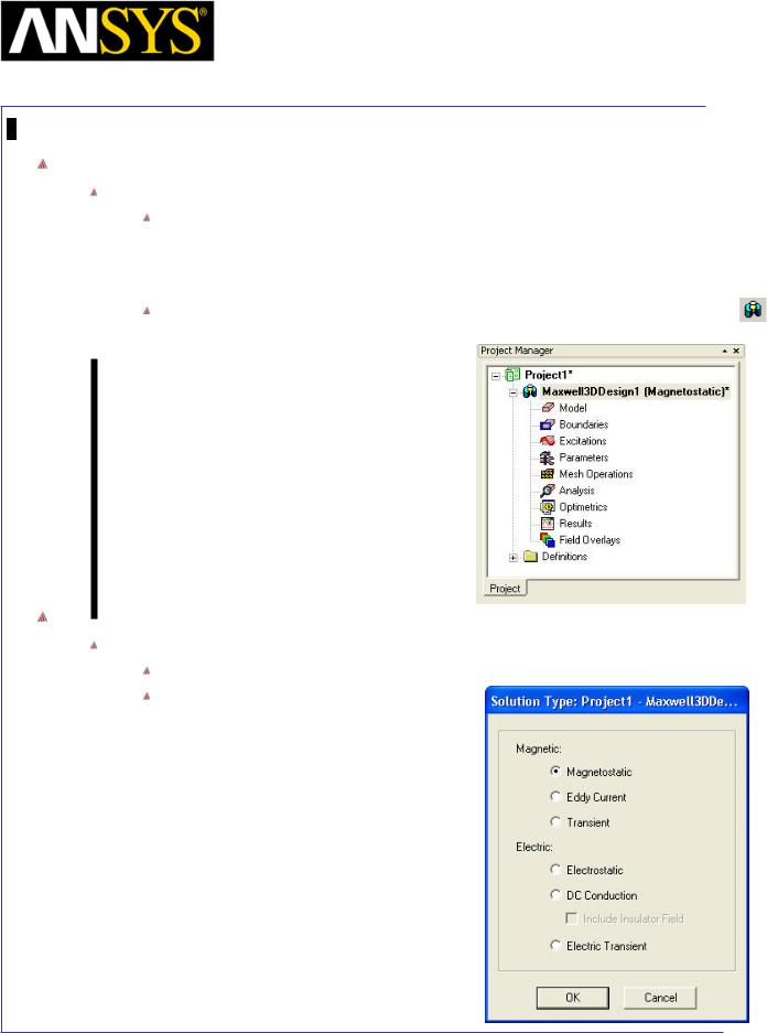
Maxwell v15 |
5.4 |
Example (Magnetostatic) – ECE: Linear Movement
Opening a New Project
To open a new project:
After launching Maxwell, a project will be automatically created. You can also create a new project using below options.
1.In an Maxwell window, click the On the Standard toolbar, or select the menu item File > New.
Select the menu item Project > Insert Maxwell 3D Design, or click on the icon
Set Solution Type
To set the Solution Type:
Select the menu item Maxwell 3D > Solution Type
Solution Type Window:
1.Choose Magnetostatic
2.Click the OK button
|
|
|
|
|
|
|
|
|
|
|
|
|
|
|
|
|
|
|
|
|
|
|
|
|
|
|
|
|
|
|
|
ANSYS Maxwell 3D Field Simulator v15 User’s Guide |
|
5.4-4 |
|||||
|
|
|
|
|
|
|
|
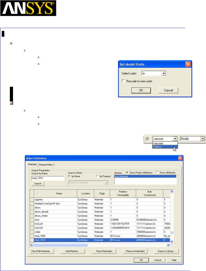
Maxwell v15 |
5.4 |
Example (Magnetostatic) – ECE: Linear Movement
Set Model Units
To Set the units:
Select the menu item Modeler > Units
Set Model Units:
1.Select Units: in (inches)
2.Click the OK button
Set Default Material
To set the default material:
Using the 3D Modeler Materials toolbar, choose Select
In Select Definition window,
1.Type steel_1010 in the Search by Name field
2.Click the OK button
|
|
|
|
|
|
|
|
|
|
|
|
|
|
|
|
|
|
|
|
|
|
|
|
|
|
|
|
|
|
|
|
ANSYS Maxwell 3D Field Simulator v15 User’s Guide |
|
5.4-5 |
|||||
|
|
|
|
|
|
|
|
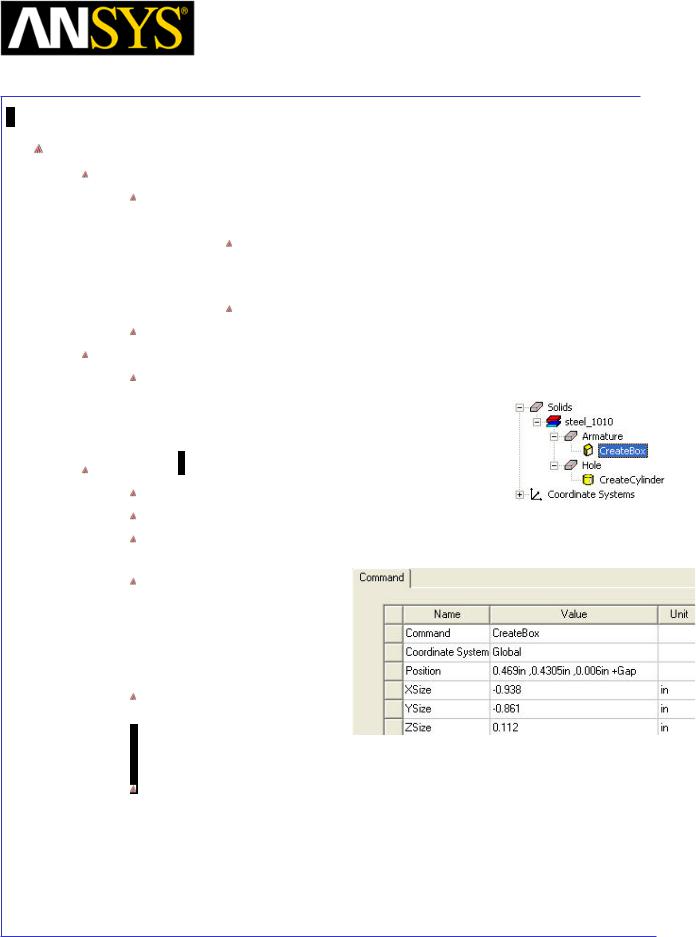
Maxwell v15 |
5.4 |
Example (Magnetostatic) – ECE: Linear Movement
Create Armature
Create Box
Select the menu item Draw > Box
1. Using the coordinate entry fields, enter the box position X: 0.469, Y: 0.4305, Z: 0.006, Press the Enter key
2.Using the coordinate entry fields, enter the opposite corner of the box:
dX: -0.938, dY: -0.861, dZ: 0.112, Press the Enter key
Select the menu item View > Fit All > Active View.
Change Attributes
Select the resulting object from the tree and goto Properties window
1.Change the name of the object to Armature
2.Change its color to Purple
Parameterize Armature
Expand the history tree of the object Armature Double click on the command CreateBox from the tree
For Position, type: 0.469, 0.4305, 0.006in +Gap, Click the Tab key to accept
In Add variable window,
1.Unit Type: Length
2.Unit: in (inches)
3.Value: 0
4.Press OK
Press OK to exit
Note: We will first run a nominal calculation with value of Gap=0. Then we will setup a parametric sweep to very Gap value over a range and check its effect on output parameters.
|
|
|
|
|
|
|
|
|
|
|
|
|
|
|
|
|
|
|
|
|
|
|
|
|
|
|
|
|
|
|
|
ANSYS Maxwell 3D Field Simulator v15 User’s Guide |
|
5.4-6 |
|||||
|
|
|
|
|
|
|
|
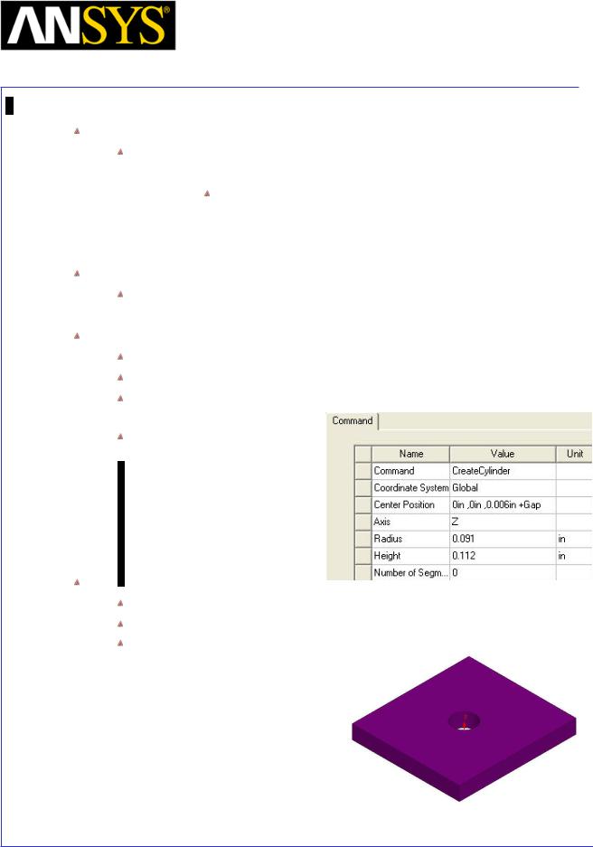
Maxwell v15 |
5.4 |
Example (Magnetostatic) – ECE: Linear Movement
Create Hole
Select the menu item Draw > Cylinder
1. Using the coordinate entry fields, enter the centre of base X: 0.0, Y: 0.0, Z: 0.006, Press the Enter key
2.Using the coordinate entry fields, enter the radius and height of cylinder
 dX: 0.091, dY: 0.0, dZ: 0.112, Press the Enter key Change Attributes
Select the resulting object from the tree and goto Properties window 1. Change the name of the object to Hole
Parameterize Hole
Expand the history tree of the object Hole
Double click on the command CreateCylinder from the tree
For Position, type: 0.469, 0.4305, 0.006in +Gap, Click the Tab key to accept
Press OK to exit
Subtract Hole
Press Ctrl and select the objects Armature and Hole from the tree
Select the menu item Modeler > Boolean > Subtract
In Subtract Window,
1.Blank Parts: Armature
2.Tool Parts: Hole
3.Click the OK button
|
|
|
|
|
|
|
|
|
|
|
|
|
|
|
|
|
|
|
|
|
|
|
|
|
|
|
|
|
|
|
|
ANSYS Maxwell 3D Field Simulator v15 User’s Guide |
|
5.4-7 |
|||||
|
|
|
|
|
|
|
|
|
|
|
Maxwell v15 |
|
5.4 |
||
|
|
Example (Magnetostatic) – ECE: Linear Movement |
|||||
|
|
|
|
|
|
|
|
|
|
Create Stator |
|
|
|
|
|
|
|
|
|
|
|
|
|
|
|
|
|
|
|
|
|
|
|
Create Profile for Sweep |
|
|
|
||
|
|
Select the menu item Draw > Line |
|
|
|
||
1. |
Using the coordinate entry field, enter the first point of the line |
|
|
|
|||
|
|
|
X: 0.5025, Y: 0.0, Z: 0.0, Press the Enter key |
|
|
|
|
2. |
Using the coordinate entry field, enter the second point of the line |
||||||
|
|
|
X: 0.5025, Y: 0.168, Z:0.0, Press the Enter key |
|
|
|
|
3. |
Using the coordinate entry field, enter the next point of the line |
|
|
|
|||
|
|
|
X: 0.5025, Y: 0.168, Z:-0.803, Press the Enter key |
|
|
|
|
4. |
Using the coordinate entry field, enter the next point of the line |
|
|
|
|||
|
|
|
X: 0.5025, Y: 0.324, Z:-0.803, Press the Enter key |
|
|
|
|
5. |
Using the coordinate entry field, enter the next point of the line |
|
|
|
|||
|
|
|
X: 0.5025, Y: 0.324, Z:0.0, Press the Enter key |
|
|
|
|
6. |
Using the coordinate entry field, enter the next point of the line |
|
|
|
|||
|
|
|
X: 0.5025, Y: 0.5, Z:0.0, Press the Enter key |
|
|
|
|
7. |
Using the coordinate entry field, enter the next point of the line |
|
|
|
|||
|
|
|
X: 0.5025, Y: 0.5, Z:-0.98, Press the Enter key |
|
|
|
|
8. |
Using the coordinate entry field, enter the next point of the line |
|
|
|
|||
|
|
|
X: 0.5025, Y: -0.5, Z:-0.98, Press the Enter key |
|
|
|
|
9. |
Using the coordinate entry field, enter the next point of the line |
|
|
|
|||
|
|
|
X: 0.5025, Y: -0.5, Z:0.0, Press the Enter key |
|
|
|
|
10. |
Using the coordinate entry field, enter the next point of the line |
|
|
|
|||
|
|
|
X: 0.5025, Y: -0.324, Z:0.0, Press the Enter key |
|
|
|
|
11. |
Using the coordinate entry field, enter the next point of the line |
|
|
|
|||
|
|
|
X: 0.5025, Y: -0.324, Z:-0.803, Press the Enter key |
|
|
|
|
12. |
Using the coordinate entry field, enter the next point of the line |
|
|
|
|||
|
|
|
X: 0.5025, Y: -0.168, Z:-0.803, Press the Enter key |
|
|
|
|
13. |
Using the coordinate entry field, enter the next point of the line |
|
|
|
|||
|
|
|
X: 0.5025, Y: -0.168, Z:0.0, Press the Enter key |
|
|
|
|
14. |
Using the coordinate entry field, enter the last point of the line |
|
|
|
|||
|
|
|
X: 0.5025, Y: 0.0, Z:0.0, Press the Enter key |
|
|
|
|
15. |
Press Enter to exit |
|
|
|
|||
|
|
Change Attributes |
|
|
|
||
|
|
Select the object Polyline1 from the tree and goto Properties window |
|
|
|
||
1. |
Change the name of the object to Stator |
|
|
|
|||
2. |
Change its color to Orange |
|
|
|
|||
|
|
|
|
|
|
|
|
|
|
|
|
|
|
|
|
ANSYS Maxwell 3D Field Simulator v15 User’s Guide |
5.4-8 |
||
|
|
|
|
Maxwell v15 |
5.4 |
Example (Magnetostatic) – ECE: Linear Movement
Sweep Profile
Select the object Stator from the history tree
Select the menu item Draw > Sweep >Along Vector
1. Using the coordinate entry field, enter the first point of the vector
X: 0.5025, Y: 0.0, Z:0.0, Press the Enter key
2. Using the coordinate entry field, enter the last point of the vector (Note that the following coordinates are ABSOLUTE)
X: 0.091, Y: 0.0, Z:0.0, Press the Enter key.
Create Mirror
Select the object Stator from the history tree
Select the menu item Edit > Duplicate > Mirror
1.Using the coordinate entry field, enter the anchor point of mirror plane
X: 0.0, Y: 0.0, Z:0.0, Press the Enter key
2.Using the coordinate entry field, enter the target point of vector normal to the mirror plane
dX: -1, dY: 0.0, dZ:0.0, Press the Enter key
|
|
|
|
|
|
|
|
|
|
|
|
|
|
|
|
|
|
|
|
|
|
|
|
|
|
|
|
|
|
|
|
ANSYS Maxwell 3D Field Simulator v15 User’s Guide |
|
5.4-9 |
|||||
|
|
|
|
|
|
|
|

Maxwell v15 |
5.4 |
Example (Magnetostatic) – ECE: Linear Movement
Set Default Material
To set the default material:
Using the 3D Modeler Materials toolbar, choose Select
In Select Definition window,
1.Type copper in the Search by Name field
2.Click the OK button
Create Coil
Create Box
Select the menu item Draw >Box
1. Using the coordinate entry fields, enter the box position X: -0.646, Y: -0.264, Z: -0.803, Press the Enter key
2.Using the coordinate entry fields, enter the opposite corner of the box:
dX: 1.292, dY: 0.528, dZ: 0.511, Press the Enter key
Change Attributes
Select the resulting object from the tree and goto Properties window
1.Change the name of the object to Coil
2.Change its color to Blue
Create another Box
Select the menu item Draw >Box
1. Using the coordinate entry fields, enter the box position X: -0.55, Y: -0.168, Z: -0.803, Press the Enter key
2.Using the coordinate entry fields, enter the opposite corner of the box:
 dX: 1.1, dY: 0.336, dZ: 0.511, Press the Enter key Change Attributes
Select the resulting object from the tree and goto Properties window 1. Change the name of the object to BaseCoil
|
|
|
|
|
|
|
|
|
|
|
|
|
|
|
|
|
|
|
|
|
|
|
|
|
|
|
|
|
|
|
|
ANSYS Maxwell 3D Field Simulator v15 User’s Guide |
|
5.4-10 |
|||||
|
|
|
|
|
|
|
|
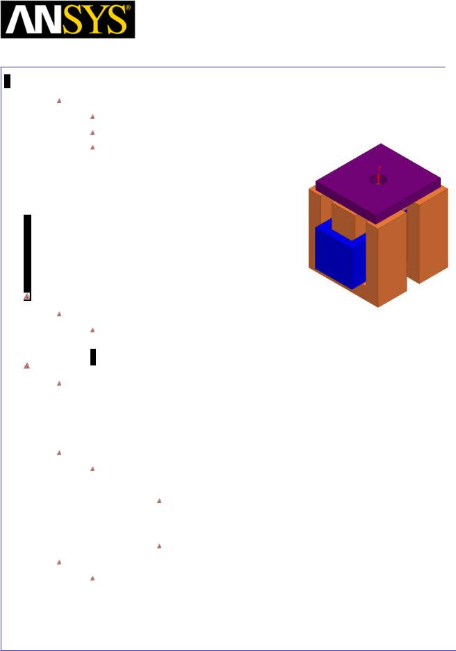
Maxwell v15 |
5.4 |
Example (Magnetostatic) – ECE: Linear Movement
Subtract Hole
Press Ctrl and select the objects Coil and BaseCoil from the tree
Select the menu item Modeler > Boolean > Subtract
In Subtract Window,
1.Blank Parts: Coil
2.Tool Parts: BaseCoil
3.Click the OK button
Set Default Material
To Set Default Material
Using the 3D Modeler Materials toolbar, choose Vacuum
Create Band Region
Note: During parametric sweep, we will very the location of armature, thus moving it in positive or negative Z direction. In such cases, it is advisable to create a Box (Band Region) around the moving object to help mesh creation. (Band Region is usually created with Transient solver to specify Object motion. But it is good to follow same process even for Magnetostatic simulation).
To Create Band Region
Select the menu item Draw >Box
1. Using the coordinate entry fields, enter the box position X: -0.55, Y: -0.55, Z: 0.003, Press the Enter key
2.Using the coordinate entry fields, enter the opposite corner of the box:
dX: 1.1, dY: 1.1, dZ: 0.147, Press the Enter key
Change Attributes
Select the resulting object from the tree and goto Properties window
1.Change the name of the object to Band
2.Display Wireframe: Checked
|
|
|
|
|
|
|
|
|
|
|
|
|
|
|
|
ANSYS Maxwell 3D Field Simulator v15 User’s Guide |
|
5.4-11 |
|||||
|
|
|
|
|
|
|
|
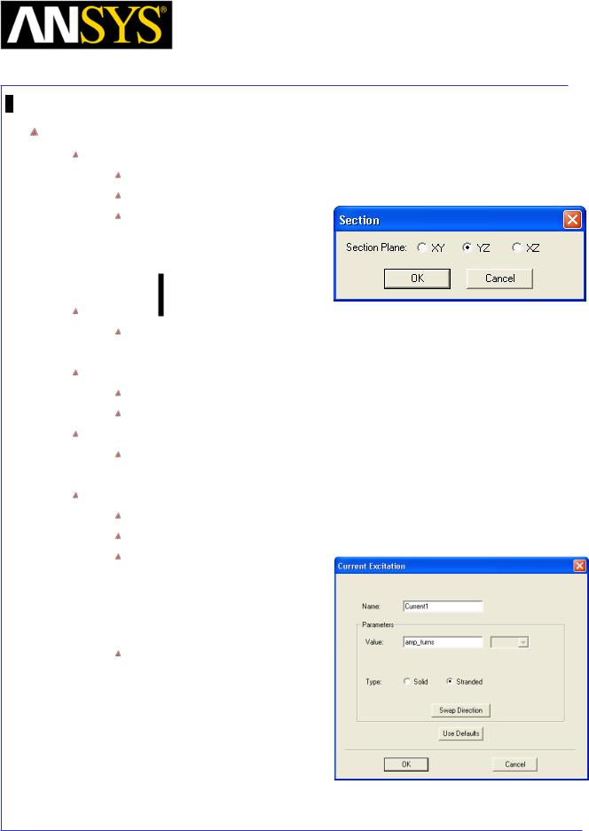
Maxwell v15 |
5.4 |
Example (Magnetostatic) – ECE: Linear Movement
Create Excitations
Create Section of coil for assigning Current
Select the object Coil from the history tree
Select the menu item Modeler > Surface > Section
In Section window,
1.Section Plane: YZ
2.Click the OK button
Change Attributes
Select the object Coil_Section1 from the tree and goto Properties window 1. Change the name of the object to Coil_Terminal
Separate Sheets
Select the sheet Coil_Terminal
Select the menu item Modeler > Boolean > Separate Bodies
Delete Extra Sheets
Select the sheet Coil_Terminal_Seperate1 from the tree
 Select the menu item Edit >Delete Assign Excitations
Select the sheet Coil_Terminal from the history tree
Select the menu item Maxwell 3D > Excitations > Assign > Current
In Current Excitation window,
1.Name: Current1
2.Value: amp_turns
3.Type: Stranded
4.Press OK
In Add variable window,
1.Unit Type: Current
2.Unit: A
3.Value: 576
4.Press OK
|
|
|
|
|
|
|
|
|
|
|
|
|
|
|
|
|
|
|
|
|
|
|
|
|
|
|
|
|
|
|
|
ANSYS Maxwell 3D Field Simulator v15 User’s Guide |
|
5.4-12 |
|||||
|
|
|
|
|
|
|
|
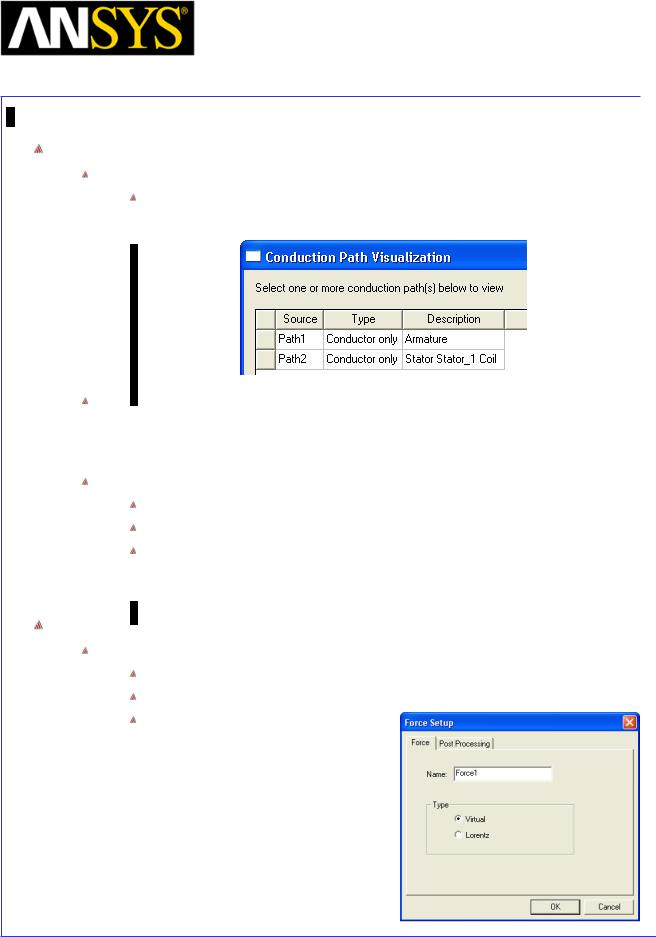
Maxwell v15 |
5.4 |
Example (Magnetostatic) – ECE: Linear Movement
Assign Boundary Conditions
Check Conduction path
Select the menu item Maxwell 3D > Excitations > Conduction Path > Show Conduction Paths
Note: We assume that no current leaks out of the coil and into the stators. However, the stators and the coil are touching which forms a conduction path from coil to both stators. Thus an insulating boundary must be applied to the either the coil or to both stators to avoid current leakage.
Assign Boundary
Press Ctrl and select the objects Stator and Stator_1 from the tree
Select the menu item Maxwell 3D > Boundaries > Assign > Insulating
In Insulating Boundary window, 1. Press OK
Assign Executive Parameters
Assign Force Parameter
Select the object Armature from the history tree
Select the menu item Maxwell 3D > Parameters > Assign > Force
In Force Setup window,
1.Name: Force1
2.Type: Virtual
3.Press OK
|
|
|
|
|
|
|
|
|
|
|
|
ANSYS Maxwell 3D Field Simulator v15 User’s Guide |
|
5.4-13 |
|||
|
|
|
|
|
|
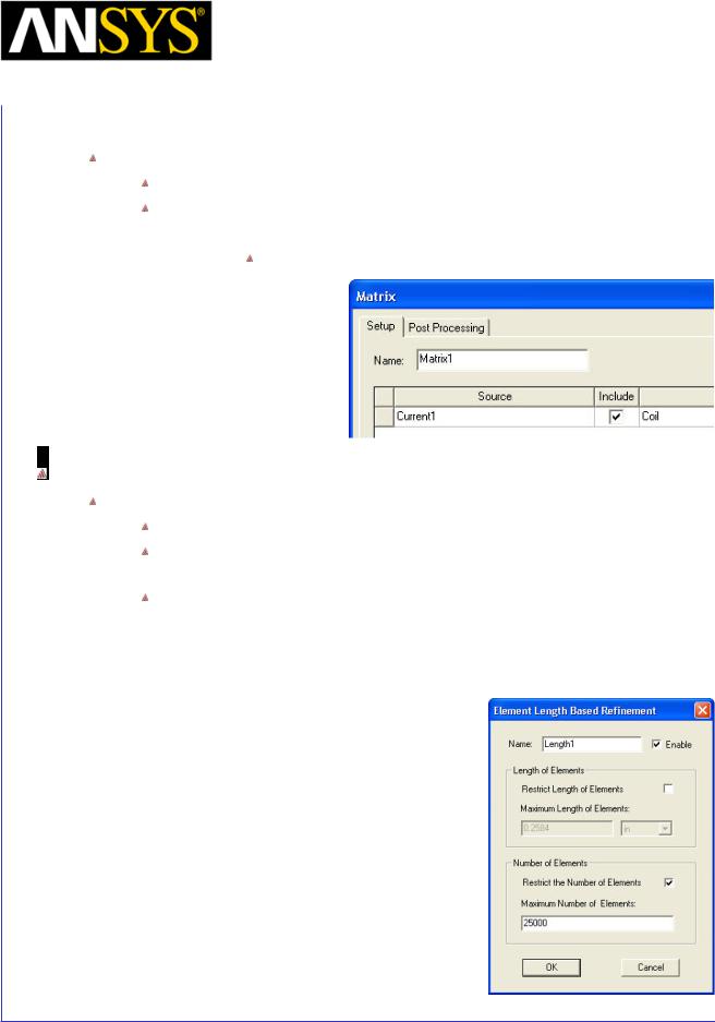
|
|
|
|
|
Maxwell v15 |
5.4 |
|
|
|
Example (Magnetostatic) – ECE: Linear Movement |
|||||
|
|
|
|
|
|
|
|
|
|
Assign Matrix |
|
|
|||
|
|
|
|
||||
|
|
|
|
||||
|
|
|
|
Select menu item Maxwell 3D > Parameters > Assign > Matrix |
|
|
|
|
|
|
|
In Matrix window, |
|
|
|
1. |
Solver Tab: |
|
|
||||
|
|
|
|
|
Include : Checked for source Current1 |
|
|
2. |
Press OK |
|
|
||||
|
|
|
|
|
|
|
|
|
|
|
|
|
|
|
|
Assign Mesh Operations
To Apply Mesh Operations
Select the menu item Edit > Select All
Select the menu item Maxwell 3D > Mesh Operations >Assign > Inside
Selection > Length Based
In Element Length Based Refinement window,
1.Restrict Length of Elements: Unchecked
2.Restrict the Number of Elements: Checked
3.Maximum Number of Elements: 25000
|
|
|
|
|
|
|
|
|
|
|
|
|
|
|
|
|
|
|
|
|
|
|
|
|
|
|
|
|
|
|
|
ANSYS Maxwell 3D Field Simulator v15 User’s Guide |
|
5.4-14 |
|||||
|
|
|
|
|
|
|
|
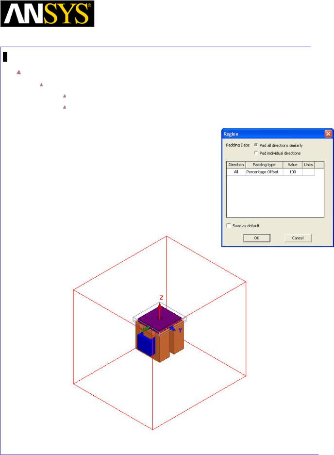
Maxwell v15 |
5.4 |
Example (Magnetostatic) – ECE: Linear Movement
Define Region
Create Simulation Region
Select the menu item Draw > Region
In Region window,
1.Pad all directions similarly: Checked
2.Padding Type: Percentage Offset
3.Value: 100
4.Press OK
|
|
|
|
|
|
|
|
|
|
|
|
ANSYS Maxwell 3D Field Simulator v15 User’s Guide |
|
5.4-15 |
|||
|
|
|
|
|
|
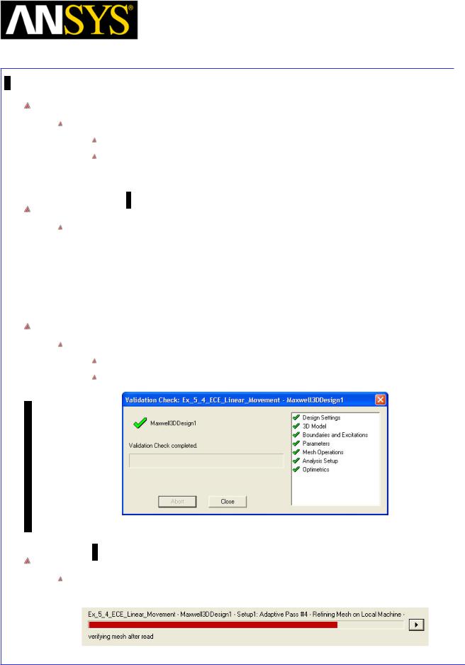
Maxwell v15 |
5.4 |
Example (Magnetostatic) – ECE: Linear Movement
Analysis Setup
To create an analysis setup:
Select the menu item Maxwell 3D > Analysis Setup > Add Solution Setup
Solution Setup Window:
1. Click the OK button to accept all default settings.
Save Project
To save the project:
1.In an Ansoft Maxwell window, select the menu item File > Save As.
2.From Save As window, type the Filename: Ex_5_4_ECE_Linear_Movement
3.Click the Save button
Model Validation
To validate the model:
Select the menu item Maxwell 3D > Validation Check
Click the Close button
Note: To view any errors or warning messages, use the Message Manager.
Analyze
To start the solution process:
1. Select the menu item Maxwell 3D > Analyze All
|
|
|
|
|
|
|
|
|
|
|
|
|
|
|
|
|
|
|
|
|
|
|
|
|
|
|
|
|
|
|
|
ANSYS Maxwell 3D Field Simulator v15 User’s Guide |
|
5.4-16 |
|||||
|
|
|
|
|
|
|
|
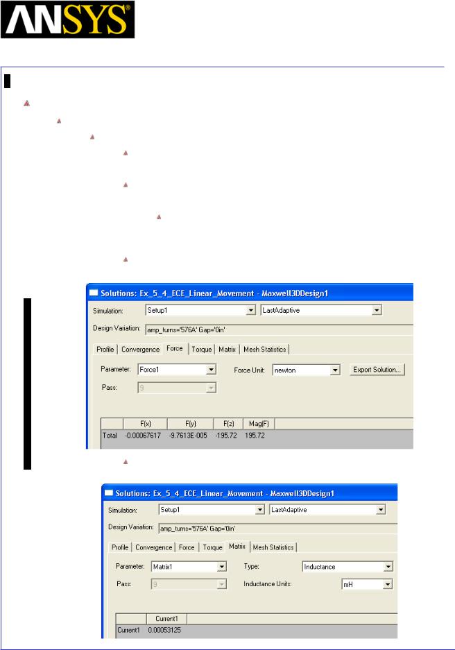
Maxwell v15 |
5.4 |
Example (Magnetostatic) – ECE: Linear Movement
Solution Data
To view the Solution Data:
Select the menu item Maxwell 3D > Results > Solution Data
To view the Profile:
1. Click the Profile Tab. To view the Convergence:
1. Click the Convergence Tab
Note: The default view is for convergence is Table. Select the Plot radio button to view a graphical representations of the convergence data.
To view the Force values: 1. Click the Force Tab
To View Inductance values 1. Click the Matrix Tab
|
|
|
|
|
|
|
|
|
|
|
|
ANSYS Maxwell 3D Field Simulator v15 User’s Guide |
|
5.4-17 |
|||
|
|
|
|
|
|
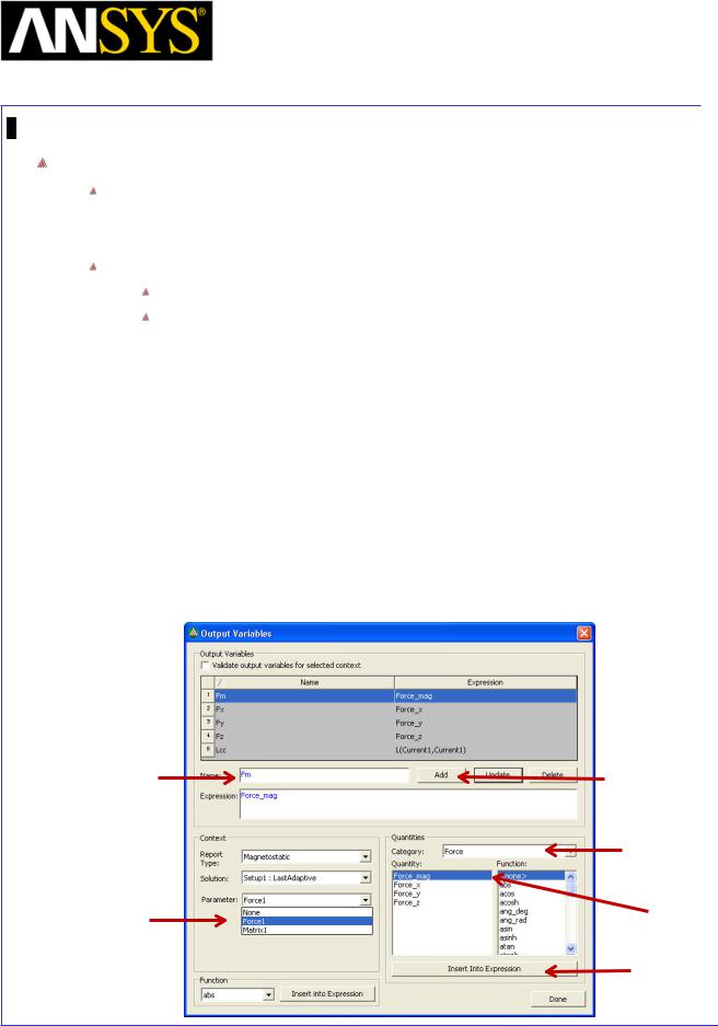
Maxwell v15 |
5.4 |
Example (Magnetostatic) – ECE: Linear Movement
Setup the Parametric Analysis for ECE
The ECE model will have two input and two output variables
1.Input: amp_turns and Gap (variables already defined)
2.Output: Armature Force and Coil Inductance (need to create variables)
To Create Output Variables
Select the menu item Maxwell 3D > Results > Output Variables
In Output Variables window,
1.Parameter: Force1
2.Category: Force
3.Qunatity: Force_mag
4.Select the buttom Insert Into Expression
5.Specify the name as Fm and select Add
6.Similarly create variables Fx, Fy and Fz for Force_x, Force_y and Force_z respectively
7.Change the Parameter to Matrix
8.Change Category to L and Quantity to L(Current1, Current1) and select the button Insert Into Expression
9.Specify the name as Lcc and select Add
10.Press Done to close window
5. Set the |
|
|
|
|
|
|
|
|
|
|
|
|
|
6. Press Add |
||
|
|
|
|
|
|
|
|
|
|
|
|
|
||||
Name |
|
|
|
|
|
|
|
|
|
|
|
|
|
|||
|
|
|
|
|
|
|
|
|
|
|
|
|
|
|
|
|
|
|
|
|
|
|
|
|
|
|
|
|
|
|
2. Select |
||
|
|
|
|
|
|
|
|
|
|
|
|
|
|
Category |
||
1. Select |
|
|
|
|
|
|
|
|
|
|
|
|
|
3. Select |
||
|
|
|
|
|
|
|
|
|
|
|
|
|
||||
|
|
|
|
|
|
|
|
|
|
|
|
|
||||
|
|
|
|
|
|
|
|
|
|
|
|
|
||||
|
|
|
|
|
|
|
|
|
|
|||||||
Parameter |
|
|
|
|
|
|
|
|
|
|
|
|
|
Quantity |
||
|
|
|
||||||||||||||
|
|
|
|
|
|
|
|
|
|
|
|
|
|
|
|
|
|
|
|
|
|
|
|
|
|
|
|
|
|
|
4. Select |
||
|
|
|
|
|
|
|||||||||||
|
|
|
|
|
|
|
|
|
|
|
|
|
|
the Button |
||
|
|
|
|
|
|
|
|
|
|
|
|
|
|
|
|
|
|
|
|
|
|
|
|
|
|
|
|
|
|
|
|
|
|
ANSYS Maxwell 3D Field Simulator v15 User’s Guide |
5.4-18 |
||
|
|
|
|
Maxwell v15 |
5.4 |
Example (Magnetostatic) – ECE: Linear Movement
Create Parametric Sweep
To Create Parametric Sweep
Select the menu item Maxwell 3D > Optimetrics Analysis > Add Parametric
In Setup Sweep Analysis window, on the Sweep Definitions tab, click the Add button
Add/Edit Sweep Dialog
1.Select Variable: Gap
2.Select Linear Step
3.Start: 0
4.Stop: 0.006
5.Step: 0.001
6.Click Add
7.Change Variable to amp_turns
8.Change the option to Single Value
9.Specify Value of -1
10.Click Add
11.Follow previous three steps again for values of 330A, 661A and 992 A
12.Press OK to return to Setup Sweep Analysis window
|
|
|
|
|
|
|
|
|
|
|
|
|
|
|
|
|
|
|
|
|
|
|
|
|
|
|
|
|
|
|
|
|
|
|
|
|
|
|
|
|
|
|
|
|
|
|
|
|
|
ANSYS Maxwell 3D Field Simulator v15 User’s Guide |
|
5.4-19 |
|||||||
|
|
|
|
|
|
|
|
|
|
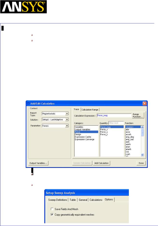
Maxwell v15 |
5.4 |
Example (Magnetostatic) – ECE: Linear Movement
Select Calculations tab, select Setup Calculations
In Add/Edit Calculation window,
1.Parameter: Force1
2.Category: Output Variables
3.Quantity: Fm
4.Click on Add Calculation
5.Repeat same steps for Fx, Fy and Fz
6.Change Parameter to Matrix1
7.Category: Output Variables
8.Quantity: Lcc
9.Click on Add Calculation
10.Press Done
On Options tab
1. Copy geometrically equivalent meshes: Checked Press OK to close window
|
|
|
|
|
|
|
|
|
|
|
|
|
|
|
|
|
|
|
|
|
|
|
|
|
|
|
|
|
|
|
|
|
|
|
|
|
|
|
|
|
|
|
|
|
|
|
|
|
|
ANSYS Maxwell 3D Field Simulator v15 User’s Guide |
|
5.4-20 |
|||||||
|
|
|
|
|
|
|
|
|
|
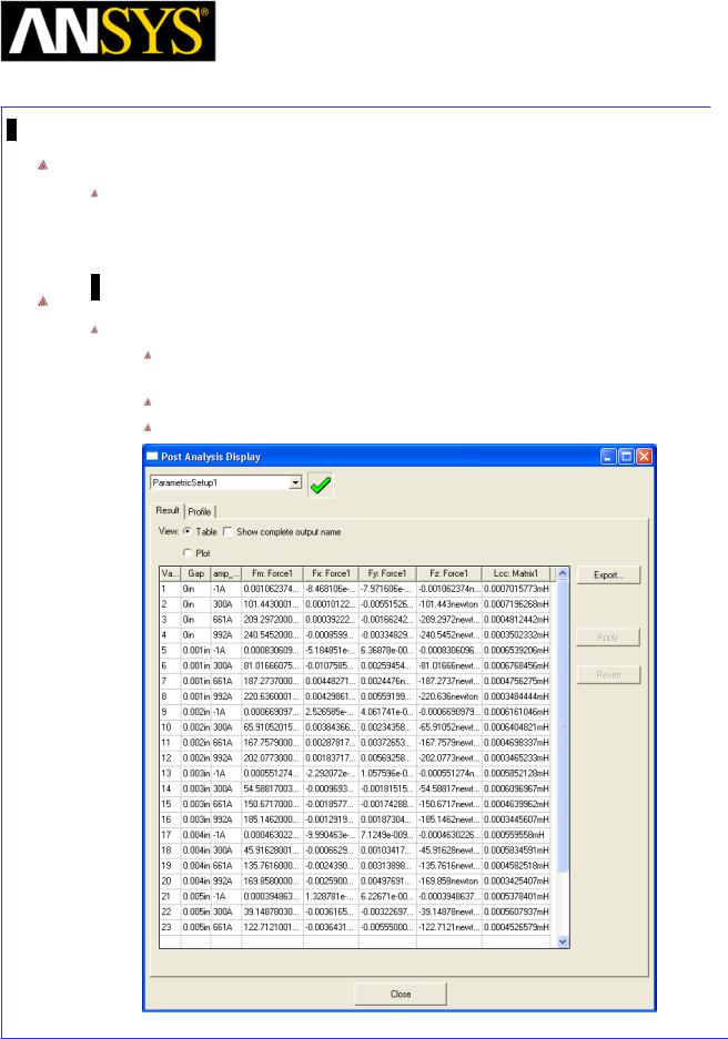
Maxwell v15 |
5.4 |
Example (Magnetostatic) – ECE: Linear Movement
Analyze Parametric Sweep
To start the solution process:
1.Expand the Project Tree to display the items listed under Optimetrics
2.Right-click the mouse on ParametricSetup1 and choose Analyze
Solution Data for Parametric Sweep
To view the Optimetrics Results:
Select the menu item Maxwell 3D > Optimetrics Analysis > Optimetrics Results
Select the Profile Tab to view the solution progress for each setup. Click the Close button when you are finished viewing the results
|
|
|
|
|
|
|
|
|
|
|
|
|
|
|
|
|
|
|
|
|
|
|
|
|
|
|
|
|
|
|
|
ANSYS Maxwell 3D Field Simulator v15 User’s Guide |
|
5.4-21 |
|||||
|
|
|
|
|
|
|
|
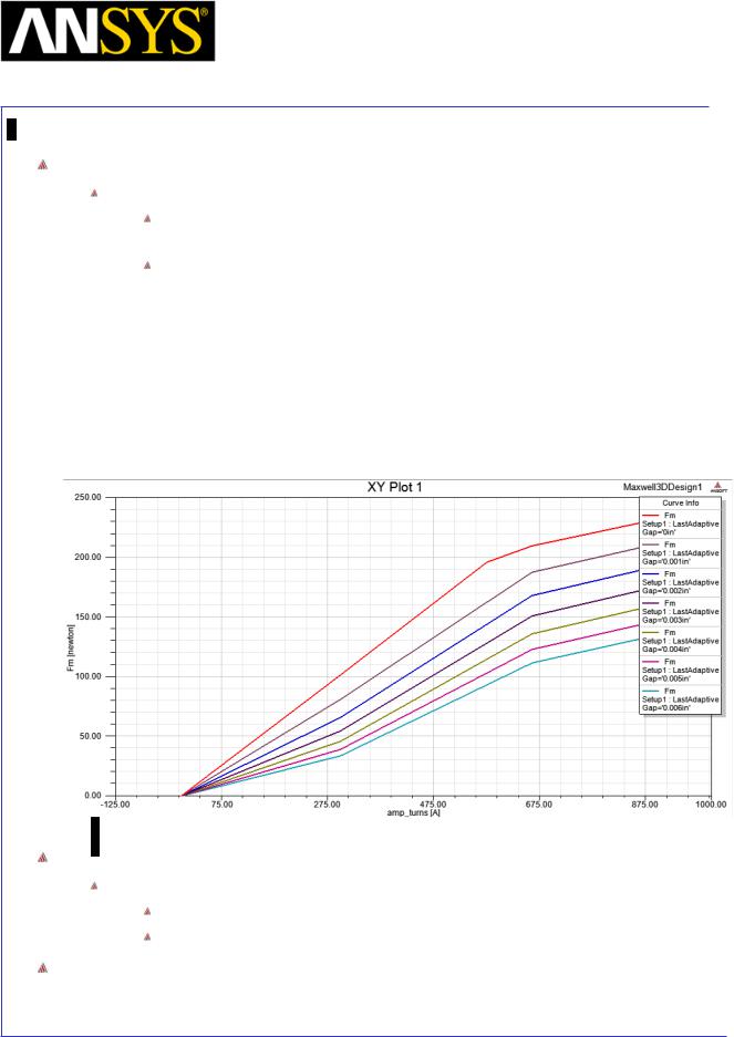
Maxwell v15 |
5.4 |
Example (Magnetostatic) – ECE: Linear Movement
Create Plot of Force Vs Current for each Gap
To create a report:
Select the menu item Maxwell 3D > Results > Create Magnetostatic Report > Rectangular Plot
In Report window,
1.Solution: Setup1: LastAdaptive
2.Parameter: Force1
3.Primary Sweep: amp_turns
4.X: Default
5.Category: Output Variables
6.Quantity: Fm
7.Press New Report
8.Press Close
Save and Exit
To Save
Select the menu item File > Save
Select the menu item File > Exit
This concludes Maxwell part.
|
|
|
|
|
|
|
|
|
|
|
|
ANSYS Maxwell 3D Field Simulator v15 User’s Guide |
|
5.4-22 |
|||
|
|
|
|
|
|
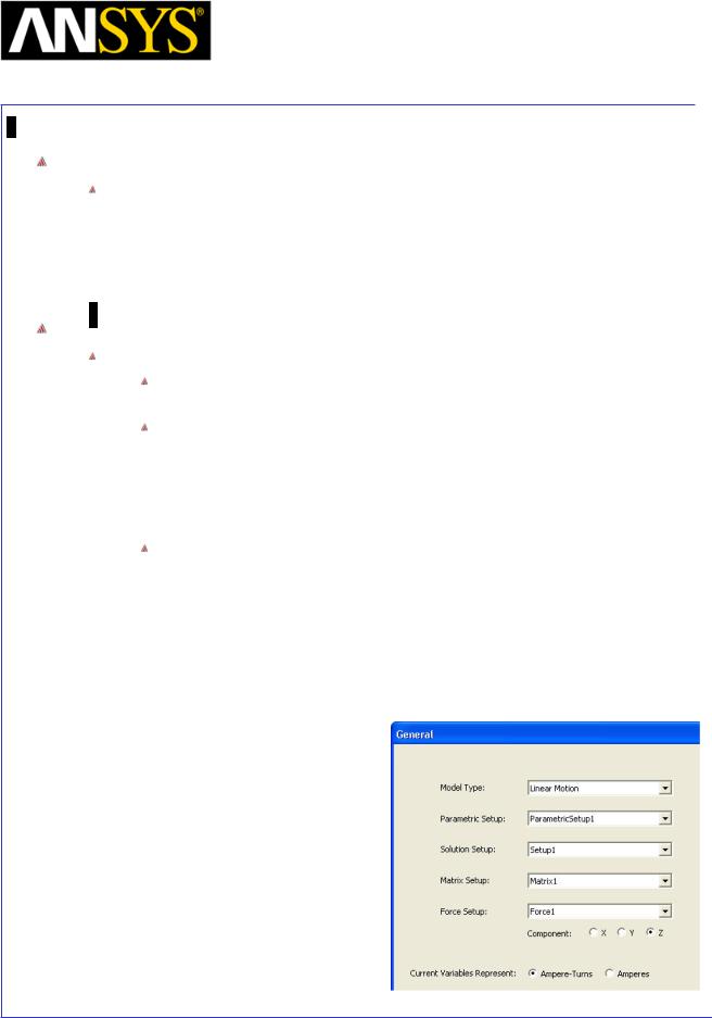
Maxwell v15 |
5.4 |
Example (Magnetostatic) – ECE: Linear Movement
ECE from the Parametric Analysis
In order to ultimately perform a system simulation in Simplorer an equivalent magnetic model must exported from Maxwell 3D. This model contains input pins for current and gap and outputs for force and flux linkage. The following steps show how to create this equivalent model. (Note: if you do not intend to do a system simulation in Simplorer, then these steps are not necessary.)
Extract Equvalent Circuit
To Extract Equivalent Circuit
Launch Simplorer and in Simplorer, select the menu item Simplorer Circuit > SubCircuit > Maxwell Component > Add Equivalent Circuit
In Maxwell Equivalent Circuit Model window,
1.Source Project File: Browse to the location of saved Maxwell Project file and select it
2.Design Type: Select 3D
3.Select the Button Extract Equivalent Circuit
Maxwell will be launched and source file will open. In Maxwell window,
1.
2.
Ensure Model Type is set to Linear Motion
Under Parametric Setup, select the parametric setup for which circuit needs to extracted
3.Select the component Z as only Z component of force will be transferred
4.Select Current Variable as Ampere-Turns as we have specified ampere-turns value for current (as we specified stranded Conductor)
5.Press Next
|
|
|
|
|
|
|
|
|
|
|
|
ANSYS Maxwell 3D Field Simulator v15 User’s Guide |
|
5.4-23 |
|||
|
|
|
|
|
|
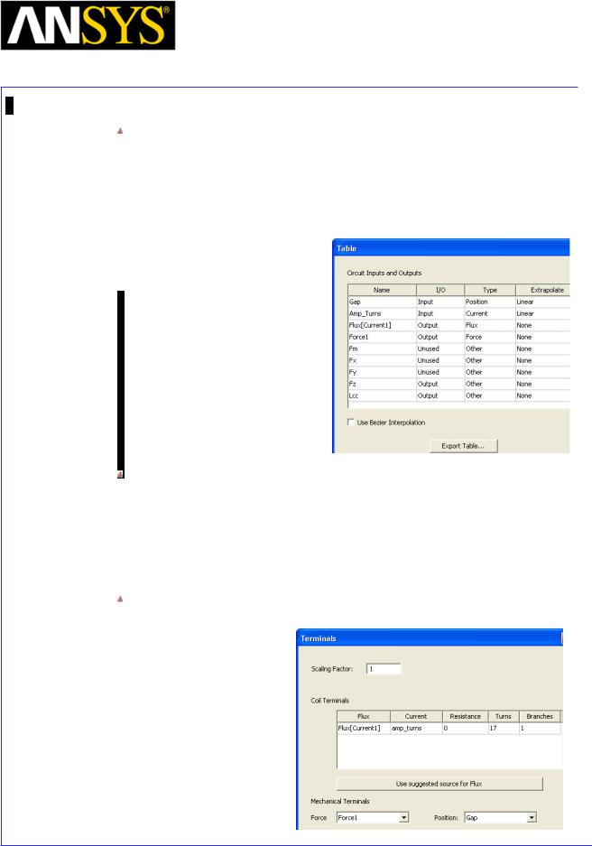
Maxwell v15 |
5.4 |
Example (Magnetostatic) – ECE: Linear Movement
In the next window
1.As the parameters Fm, Fx and Fy will not be used in simplorer circuit, change the I/O column for these parameters to Unused
2.Make sure that the data types are correct: Gap corresponds to Position and Amp_Turns corresponds to Current.
3.Optionally if data needs to be exported in tabular format, select Export Table button
4.Press Next
Next window defines the scaling factor and the Terminals of the conservative nodes in Simplorer. The conservative nodes will have their Across and Through quantities solved by Simplorer, ensuring the physical meaning of the simulation. The Flux (and therefore the EMF) is the electrical Across quantity in this case. The current is the Through quantity. In the Mechanical domain, gap is the Across quantity whereas Force1 is the Through quantity.
In Maxwell, we specified the conductor as stranded but we have not specified number of Turns. Set Turns column for Terminal as 17 and select Finish
|
|
|
|
|
|
|
|
|
|
|
|
ANSYS Maxwell 3D Field Simulator v15 User’s Guide |
|
5.4-24 |
|||
|
|
|
|
|
|
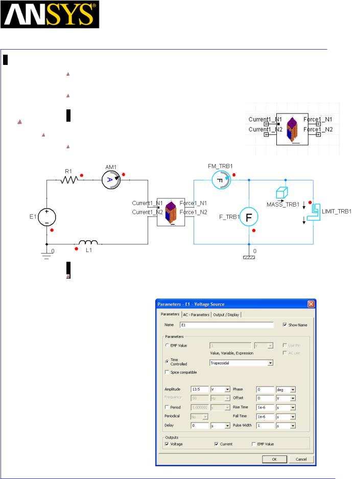
Maxwell v15 |
5.4 |
Example (Magnetostatic) – ECE: Linear Movement
Return to Simplorer window, and select OK in the Maxwell Equivalent
Circuit Model window
Place the resulting component on the Project Page
Simplorer Circuit
Build Simplorer Circuit
Build the circuit as shown in below image
Specifications of components is as below 1. Voltage Source E1
|
|
|
|
|
|
|
|
|
|
|
|
|
|
|
|
|
|
|
|
|
|
|
|
|
|
|
|
|
|
|
|
|
|
|
|
|
|
|
|
|
|
|
|
|
|
|
|
|
|
ANSYS Maxwell 3D Field Simulator v15 User’s Guide |
|
5.4-25 |
|||||||
|
|
|
|
|
|
|
|
|
|
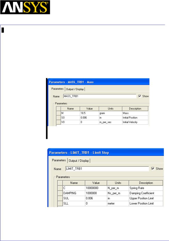
Maxwell v15 |
5.4 |
Example (Magnetostatic) – ECE: Linear Movement
2.Resistor R1, with R= 215 mOhm
3.Inductor L1, with L= 10pH
4.Ammeter AM1, for current measurement
5.Force meter FM_TRB1, for force measurement
6.Force Source F_TRB1, with F = 125 N
7.A mass MASS_TRB1 that describes the mass of the plunger of the actuator
8.A Limit stop LIMIT_TRB1 that represents a parallel damper and spring combination:
|
|
|
|
|
|
|
|
|
|
|
|
|
|
|
|
|
|
|
|
|
|
|
|
|
|
|
|
|
|
|
|
|
|
|
|
|
|
|
|
|
|
|
|
|
|
|
|
|
|
|
|
|
|
|
|
|
|
|
|
ANSYS Maxwell 3D Field Simulator v15 User’s Guide |
|
5.4-26 |
|||||||
|
|
|
|
|
|
|
|
|
|
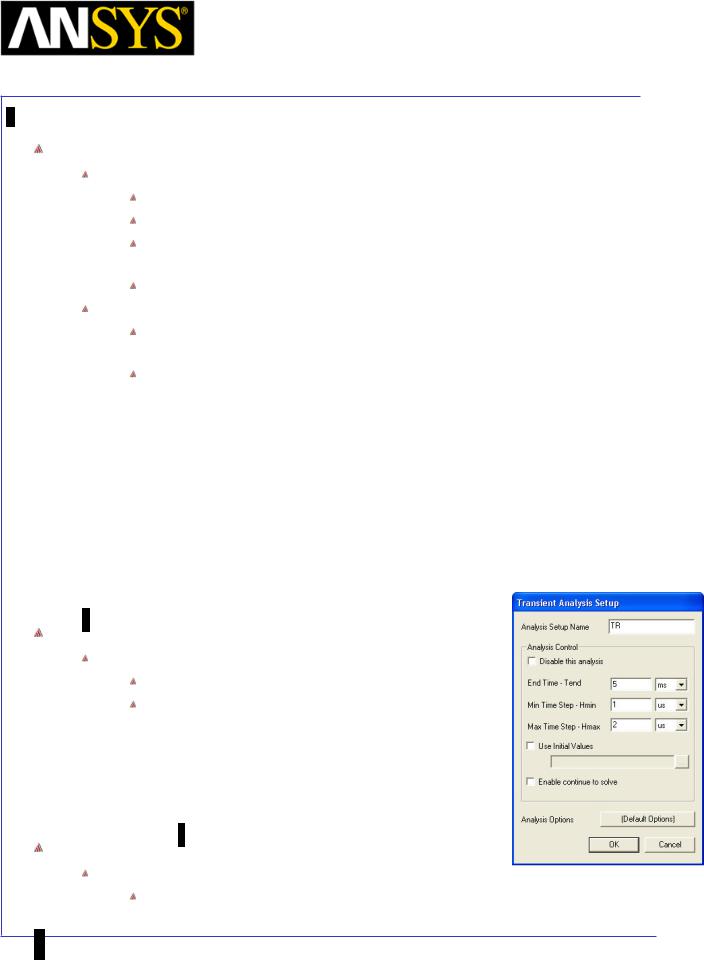
Maxwell v15 |
5.4 |
Example (Magnetostatic) – ECE: Linear Movement
Create Plots
Create ECE Parameters for Plot
Double click on ECE component from the project page
In the window, goto Quantities tab
Goto the qunatities Fz_OUT and ICurrent1 and check the box in the colum corresponding to SDB
Press OK
Create Plots
Select the menu item Simplorer Circuit > Results > Create Standard Report > Rectangular Plot
In Report window,
1.Category: All
2.Quantity: ECE1.Fz_OUT
3.Press the button New Report
4.Change Quantity to ECE1.ICurrent1
5.Press the button New Report
6.Change the Quantity to MASS.S
7.For Y type 39.79*MASS.S
8.Press the button New Report
9.Press the button Close
Create a Transient Analysis
To Create Transient Setup
Select menu item Simplorer Circuit > Edit Setup
In Transient Analysis Setup window,
1.End Time: 5 ms
2.Min. Time Step: 1 us
3.Max Time Step: 2 us
4.Press OK
Run Solution
To Run Solution
Select the menu item Simplorer Circuit > Analyze
|
|
|
|
|
|
|
|
|
|
|
|
|
|
ANSYS |
Maxwell 3D Field Simulator v15 User’s Guide |
|
5.4-27 |
|||
|
|
|
|
|
|
|
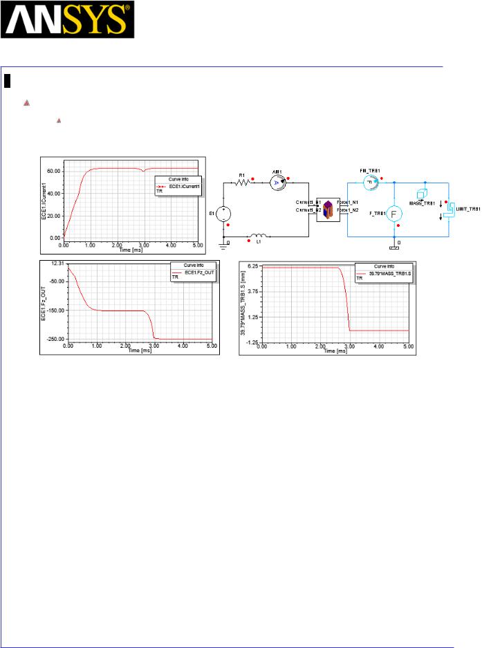
Maxwell v15 |
5.4 |
Example (Magnetostatic) – ECE: Linear Movement
Results
View Result Plots
|
|
|
|
|
|
|
|
|
|
|
|
|
|
|
|
|
|
|
|
|
|
|
|
|
|
|
|
|
|
|
|
ANSYS Maxwell 3D Field Simulator v15 User’s Guide |
|
5.4-28 |
|||||
|
|
|
|
|
|
|
|
|
Maxwell v15 |
|
5.5 |
|
Example (Magnetostatic) |
– Anisotropic Material |
|
|
|
|
|
|
|
|
|
Implementation and Application of Nonlinear Anisotropic Material
In Maxwell, Nonlinear Anisotropic Material can be used with the Magnetostatic, and Transient Solvers for simulating soft magnetic materials. The advantage is significant because
Non-linear lamination is extensively used in low frequency electromagnetic devices for having high induction but with significant reduction of eddy current loss in the rolling direction.
Non-linear anisotropy is widely used magnetization, magnetic recording, power transformers and large size electrical machines. Oriented materials will have higher magnetic field like magnetic flux density in special directions as users want but lower magnetic field in other directions.
In this note a magnetostatic model as one step of magnetization will be introduced including how to set up Non-linear lamination and Non-linear anisotropic materials.
The example that will be used to demonstrate how anisotropic non-linear material & non-linear lamination are implemented in a Magnetization model is of a fourpoles out-rotor. The intent of this write up is not how to simulate the out-rotor motors, it is rather to demonstrate how anisotropic materials are implemented within the Magnetostatic solver. This magnet ring is an non-linear anisotropic one (nonlinear in R & Z direction with low permeability in Theta direction) and the field core is a laminated one. lamination direction is Global X) Thus we can show how these materials can be set up for create an four poles out-rotor.
|
|
|
|
|
|
|
|
|
|
|
|
|
|
|
|
|
|
|
|
|
|
|
|
|
|
|
|
|
|
|
|
|
|
|
|
|
|
|
|
|
|
|
|
|
|
|
|
|
|
|
|
|
|
|
|
|
|
|
|
ANSYS Maxwell 3D Field Simulator v15 User’s Guide |
|
5.5-1 |
|||||||
|
|
|
|
|
|
|
|
|
|

|
Maxwell v15 |
|
5.5 |
|
Example (Magnetostatic) |
– Anisotropic Material |
|
|
|
|
|
|
|
|
|
ANSYS Maxwell Design Environment
The following features of the ANSYS Maxwell Design Environment are used to create the models covered in this topic
3D Solid Modeling
User Defined Primitives (UDP): RMxprt/SlotCore
Primitives: Regular Polyhedron, Box, Cylinder
Surface Operations: Section, Edge Filet
Boolean Operations: Split, Separate Bodies
Boundaries/Excitations
Current: Stranded
Analysis
Magnetostatic
Results
Field Calculator
2D plot with Create Report
Field Overlays:
Flux Density Plots
|
|
|
|
|
|
|
|
|
|
|
|
|
|
|
|
|
|
|
|
|
|
|
|
|
|
|
|
|
|
|
|
|
|
|
|
|
|
|
|
|
|
|
|
|
|
|
|
|
|
|
|
|
|
|
|
|
|
|
|
ANSYS Maxwell 3D Field Simulator v15 User’s Guide |
|
5.5-2 |
|||||||
|
|
|
|
|
|
|
|
|
|

|
Maxwell v15 |
|
5.5 |
|
Example (Magnetostatic) |
– Anisotropic Material |
|
|
|
|
|
|
|
|
|
Launching Maxwell
To access Maxwell:
1.Click the Microsoft Start button, select Programs, and select Ansoft > Maxwell 15.0 and select Maxwell 15.0
Setting Tool Options
To set the tool options:
Note: In order to follow the steps outlined in this example, verify that the following tool options are set :
1. Select the menu item Tools > Options > Maxwell 3D Options
Maxwell Options Window:
1. Click the General Options tab
Use Wizards for data input when creating new boundaries: Checked
Duplicate boundaries/mesh operations with geometry:
Checked
2.Click the OK button
2.Select the menu item Tools > Options > Modeler Options.
Modeler Options Window:
1. Click the Operation tab
 Automatically cover closed polylines: Checked 2. Click the Display tab
 Default transparency = 0.8 3. Click the Drawing tab
 Edit property of new primitives: Checked 4. Click the OK button
|
|
|
|
|
|
|
|
|
|
|
|
|
|
|
|
|
|
|
|
|
|
|
|
|
|
|
|
|
|
|
|
ANSYS Maxwell 3D Field Simulator v15 User’s Guide |
|
5.5-3 |
|||||
|
|
|
|
|
|
|
|
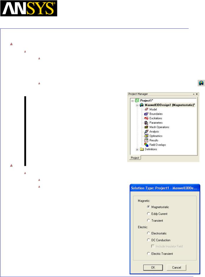
|
Maxwell v15 |
|
5.5 |
|
Example (Magnetostatic) |
– Anisotropic Material |
|
|
|
|
|
|
|
|
|
Opening a New Project
To open a new project:
After launching Maxwell, a project will be automatically created. You can also create a new project using below options.
1.In an Maxwell window, click the On the Standard toolbar, or select the menu item File > New.
Select the menu item Project > Insert Maxwell 3D Design, or click on the icon
Set Solution Type
To set the Solution Type:
Select the menu item Maxwell 3D > Solution Type
Solution Type Window:
1.Choose Magnetostatic
2.Click the OK button
|
|
|
|
|
|
|
|
|
|
|
|
|
|
|
|
|
|
|
|
|
|
|
|
|
|
|
|
|
|
|
|
|
|
|
|
|
|
|
|
|
|
|
|
|
|
|
|
|
|
|
|
|
|
|
|
|
|
|
|
ANSYS Maxwell 3D Field Simulator v15 User’s Guide |
|
5.5-4 |
|||||||
|
|
|
|
|
|
|
|
|
|
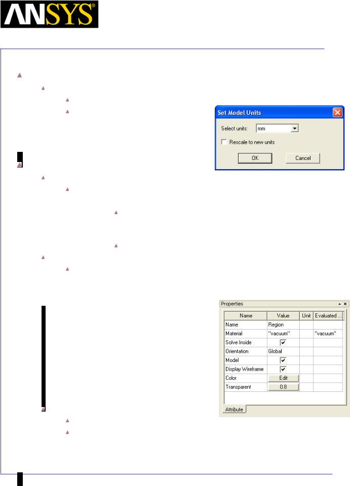
|
Maxwell v15 |
|
5.5 |
|
Example (Magnetostatic) |
– Anisotropic Material |
|
|
|
|
|
|
|
|
|
Set Model Units
To Set the units:
Select the menu item Modeler > Units
Set Model Units:
1.Select Units: mm
2.Click the OK button
Create Region
Create a Box region
Select the menu item Draw > Box or click on the icon.
icon.
1. Using the coordinate entry field, enter the box position X: -50, Y: -50, Z: -50 Press the Enter key
2.Using the coordinate entry fields, enter the opposite corner of the box:
dX: 100, dY: 100, dZ: 100, Press the Enter key
Change Attributes
Select the resulting object from the tree and goto Properties window
1.Change the name of the object to Region
2.Display Wireframe: Checked
Hide Region
Select Region from the history tree
Select the menu item View > Visibility> Hide Selection > Active View
|
|
|
|
|
|
|
|
|
|
|
|
|
|
|
|
|
|
|
|
|
|
|
|
|
|
|
ANSYS |
Maxwell 3D Field Simulator v15 User’s Guide |
|
5.5-5 |
|||||
|
|
|
|
|
|
|
|
|
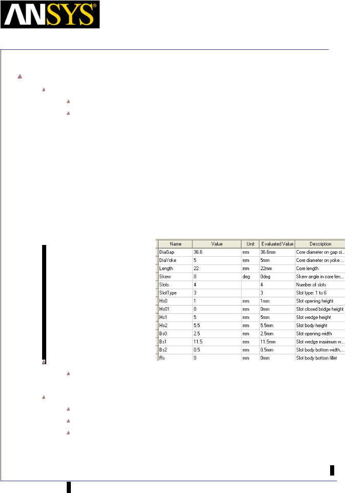
|
Maxwell v15 |
|
5.5 |
|
Example (Magnetostatic) |
– Anisotropic Material |
|
|
|
|
|
|
|
|
|
Create Field Core
To Create Core
Select Draw > User Defined Primitive > SysLib > RMxprt > SlotCore
In User Defined Primitive Operation window
1.For the value of DiaGap, type: 36.6, Click the Tab key to accept
2.For the value of DiaYoke, type: 5, Click the Tab key to accept
3.For the value of Length, type: 22, Click the Tab key to accept
4.For the value of Slots, type: 4, Click the Tab key to accept
5.For the value of SlotType, type: 3, Click the Tab key to accept
6.For the value of Hs1, type: 5, Click the Tab key to accept
7.For the value of Hs2, type: 5.5, Click the Tab key to accept
8.For the value of Bs1, type: 11.5, Click the Tab key to accept
9.For the value of Bs2, type: 0.5, Click the Tab key to accept
10.Click the OK button
Change Attributes
Select the resulting object from the tree and goto Properties window 1. Change the name of the object to FieldCore
Rotate FieldCore
Select the object FieldCore from the history tree
Select the menu item Edit > Arrange > Rotate
In Rotate window,
1.Set Axis to Y
2.Set Angle to 90
3. Press OK
ANSYS Maxwell 3D Field Simulator v15 User’s Guide |
5.5-6 |
||
|
|
|
|
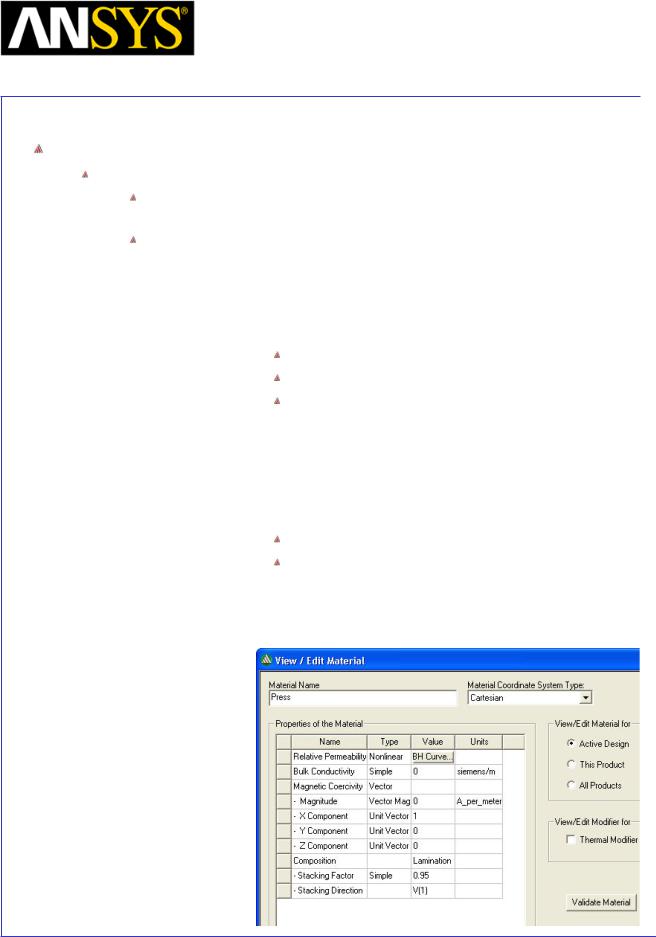
|
Maxwell v15 |
|
5.5 |
|
Example (Magnetostatic) |
– Anisotropic Material |
|
|
|
|
|
|
|
|
|
Define Material for FieldCore
To Create Material
Select the object FieldCore from the history tree, right click and select Assign Material
In Select Definition window,
1.Select option Add Material
2.In View/Edit Material window
1.Material Name Press
2.Relative Permeability
Change Type to Nonlinear
Click the BH Curve tab that will appear in Value field
In BH Curve window,
1.Select Import Dataset
2.Change File type to Tab Delimited data file
3.Locate the file Press.tab and Open it
4.Press OK to close BH Curve window
3.Composition: Change to Lamination
Stacking Factor: 0.95
Stacking Direction: V(1) [X Direction]
4.Press Validate Material
5.Press OK
3.Press OK to exit Select Definition window
|
|
|
|
|
|
|
|
|
|
|
|
ANSYS Maxwell 3D Field Simulator v15 User’s Guide |
|
5.5-7 |
|||
|
|
|
|
|
|

|
Maxwell v15 |
|
5.5 |
|
Example (Magnetostatic) |
– Anisotropic Material |
|
|
|
|
|
|
|
|
|
Create Housing
Change Grid Plane
Select the menu item Modeler > Grid Plane > YZ
Create Regular Polyhedra
Select the menu item Draw > Regular Polyhedron
1. Using the coordinate entry field, enter the center position
 X: -15.3, Y: 0, Z: 0, Press the Enter key 2. Using the coordinate entry field, enter the radius
dZ:24.4, Press the Enter key
3. Using the coordinate entry field, enter the height dX: 30.8, Press the Enter key
4.Number of Segments: 36
5.Press OK
Change Attributes
Select the resulting object from the tree and goto Properties window
1.Change the name of the object to Housing
2.Change its color to Green
Create Housing1
Select the menu item Draw > Regular Polyhedron
1. Using the coordinate entry field, enter the center position
 X: -15.3, Y: 0, Z: 0, Press the Enter key 2. Using the coordinate entry field, enter the radius
dZ:3.25, Press the Enter key
3. Using the coordinate entry field, enter the height dX: -1.7, Press the Enter key
4.Number of Segments: 16
5.Press OK
Change Attributes
Select the resulting object from the tree and goto Properties window 1. Change the name of the object to Housing1
|
|
|
|
|
|
|
|
|
|
|
|
|
|
|
|
|
|
|
|
|
|
|
|
|
|
|
|
|
|
|
|
ANSYS Maxwell 3D Field Simulator v15 User’s Guide |
|
5.5-8 |
|||||
|
|
|
|
|
|
|
|

|
Maxwell v15 |
|
5.5 |
|
Example (Magnetostatic) |
– Anisotropic Material |
|
|
|
|
|
|
|
|
|
Unite Objects
Press Ctrl and select the objects Housing and Housing1 from the tree
Select the menu item Modeler > Boolean > Unite
Create Housing2
Select the menu item Draw > Regular Polyhedron
1. Using the coordinate entry field, enter the center position
 X: -14.5, Y: 0, Z: 0, Press the Enter key 2. Using the coordinate entry field, enter the radius
dZ:22.8, Press the Enter key
3. Using the coordinate entry field, enter the height dX: 30.8, Press the Enter key
4.Number of Segments: 72
5.Press OK
Change Attributes
Select the resulting object from the tree and goto Properties window 1. Change the name of the object to Housing2
Create Housing3
Select the menu item Draw > Regular Polyhedron
1. Using the coordinate entry field, enter the center position
X: 0, Y: 0, Z: 0, Press the Enter key
2. Using the coordinate entry field, enter the radius
dZ:2.45, Press the Enter key
3. Using the coordinate entry field, enter the height dX: -20, Press the Enter key
4.Number of Segments: 16
5.Press OK
Change Attributes
Select the resulting object from the tree and goto Properties window 1. Change the name of the object to Housing3
|
|
|
|
|
|
|
|
|
|
|
|
|
|
|
|
|
|
|
|
|
|
|
|
|
|
|
|
|
|
|
|
ANSYS Maxwell 3D Field Simulator v15 User’s Guide |
|
5.5-9 |
|||||
|
|
|
|
|
|
|
|
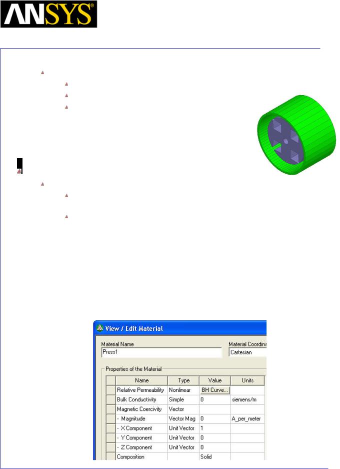
|
Maxwell v15 |
|
5.5 |
|
Example (Magnetostatic) |
– Anisotropic Material |
|
|
|
|
|
|
|
|
|
Subtract Objects
Press Ctrl and select objects Housing, Housing2 and Housing3 from tree
Select the menu it Modeler > Boolean > Subtract
In Subtract window
1.Set Housing as Blank Part
2.Set Housing2 and Housing3 as Tool Parts
3.Press OK
Define Material for Housing
To Create Material
Select the object Housing from the history tree, right click and select Assign Material
In Select Definition window,
1.Type Press in the Search by Name field
2.Select option Clone Material
3.In View/Edit Material window
1.Material Name Press1
2.Composition: Change to Solid
3.Press Validate Material
4.Press OK
4.Press OK to exit Select Definition window
|
|
|
|
|
|
|
|
|
|
|
|
|
|
|
|
|
|
|
|
|
|
|
|
|
|
|
|
|
|
|
|
ANSYS Maxwell 3D Field Simulator v15 User’s Guide |
|
5.5-10 |
|||||
|
|
|
|
|
|
|
|
|
Maxwell v15 |
|
5.5 |
|
Example (Magnetostatic) |
– Anisotropic Material |
|
|
|
|
|
|
|
|
|
Create RingMagnet
Create Regular Polyhedra
Select the menu item Draw > Regular Polyhedron
1. Using the coordinate entry field, enter the center position
X: -10, Y: 0, Z: 0, Press the Enter key
2. Using the coordinate entry field, enter the radius
dZ:22.8, Press the Enter key
3. Using the coordinate entry field, enter the height dX: 20, Press the Enter key
4.Number of Segments: 72
5.Press OK
Change Attributes
Select the resulting object from the tree and goto Properties window 1. Change the name of the object to RingMagnet and color to Red
Create Hole
Select the menu item Draw > Regular Polyhedron
1. Using the coordinate entry field, enter the center position
X: -10, Y: 0, Z: 0, Press the Enter key
2. Using the coordinate entry field, enter the radius
dZ:18.8, Press the Enter key
3. Using the coordinate entry field, enter the height dX: 20, Press the Enter key
4.Number of Segments: 72
5.Press OK
Change Attributes
Select the resulting object from the tree and goto Properties window 1. Change the name of the object to Hole
Subtract Objects
Press Ctrl and select objects RingMagnet and Hole from tree
Select the menu it Modeler > Boolean > Subtract
In Subtract window
1.Set RingMagnet as Blank Part
2.Set Hole as Tool Parts
3. Press OK
ANSYS Maxwell |
3D Field Simulator v15 User’s Guide |
5.5-11 |
||
|
|
|
|
|
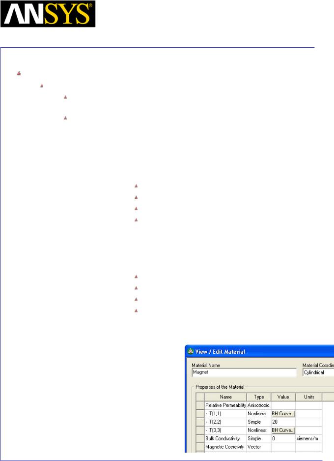
|
Maxwell v15 |
|
5.5 |
|
Example (Magnetostatic) |
– Anisotropic Material |
|
|
|
|
|
|
|
|
|
Define Material for RingMagnet
To Create Material
Select the object RingMagnet from the history tree, right click and select Assign Material
In Select Definition window,
1.Select option Add Material
2.In View/Edit Material window
1.Material Name Magnet
2.Material Coordinate System Type: Cylindrical
3.Relative Permeability
Change Type to Anisotropic
Change T(1,1) to Nonlinear
Click the BH Curve tab that will appear in Value field
In BH Curve window,
1.Select Import Dataset
2.Change File type to Tab Delimited data file
3.Locate the file Mag.tab and Open it
4.Press OK to close BH Curve window
Change value for T(2,2) to 20 Change T(3,3) to Nonlinear
Click the BH Curve tab that will appear in Value field In BH Curve window,
1. Import the same Mag.tab file
4.Press OK
3.Press OK to exit
|
|
|
|
|
|
|
|
|
|
|
|
|
|
|
|
|
|
|
|
|
|
|
|
|
|
|
|
|
|
|
|
ANSYS Maxwell 3D Field Simulator v15 User’s Guide |
|
5.5-12 |
|||||
|
|
|
|
|
|
|
|
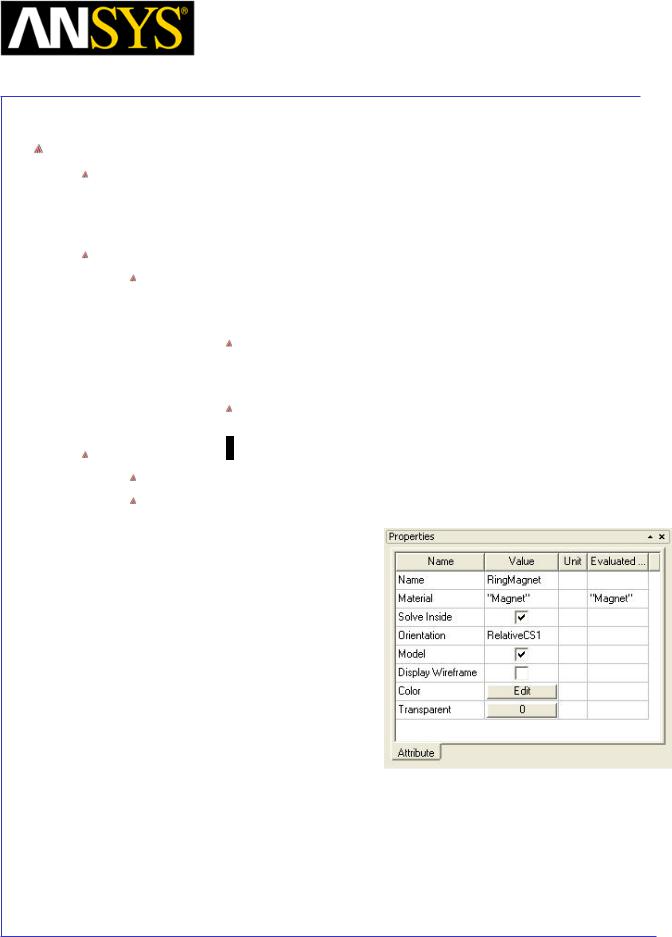
|
Maxwell v15 |
|
5.5 |
|
Example (Magnetostatic) |
– Anisotropic Material |
|
|
|
|
|
|
|
|
|
Orient RingMagnet
Note: Material created for RingMagnet is with reference to cylindrical coordinate system. In Cylindrical Coordinate System, Theta direction is fixed as T(2,2), the Global CS can’t be used for RingMagnet directly as its orientation is not along required direction. Relative Coordinate System must be created for it.
To Create Relative Coordinate System
Select the menu item Modeler > Coordinate System > Create > Relative CS > Rotated
1. Using the coordinate entry field, enter the X axis position X: 0, Y: 1, Z: 0, Press the Enter key
2.Using the coordinate entry field, enter the XY Plane position in Absolute values
X: 0, Y: 0, Z: 1, Press the Enter key
Change Orientation of Magnet
Select RingMagnet from the tree and goto Properties window
Change Orientation to RelativeCS1
|
|
|
|
|
|
|
|
|
|
|
|
|
|
|
|
|
|
|
|
|
|
|
|
|
|
|
|
|
|
|
|
ANSYS Maxwell 3D Field Simulator v15 User’s Guide |
|
5.5-13 |
|||||
|
|
|
|
|
|
|
|

|
Maxwell v15 |
|
5.5 |
|
Example (Magnetostatic) |
– Anisotropic Material |
|
|
|
|
|
|
|
|
|
Create Coil
Change Work Coordinate System
Goto Modeler > Coordinate System > Set Working CS
In Select Coordinate System Window
1.Select Global
2.Press Select
Create Box
Select the menu item Draw > Box
1. Using the coordinate entry fields, enter the box position X: 14.2, Y: 6.2, Z: -7.8, Press the Enter key
2.Using the coordinate entry fields, enter the opposite corner of the box:
dX: -28.2, dY: 6.5, dZ: 15.6, Press the Enter key
Change Attributes
Select the object from the tree and goto Properties window
1.Change the name of the object to CoilA
2.Change its color to Orange
Create CoilA_1
Select the menu item Draw > Box
1. Using the coordinate entry fields, enter the box position X: 11.2, Y: 6.2, Z: -4.8, Press the Enter key
2.Using the coordinate entry fields, enter the opposite corner of the box:
 dX: -22.4, dY: 6.5, dZ: 9.6, Press the Enter key Change Attributes
Select the object from the tree and goto Properties window 1. Change the name of the object to CoilA_1
Subtract Objects
Press Ctrl and select objects CoilA and CoilA_1 from tree
Select the menu it Modeler > Boolean > Subtract
In Subtract window
1.Set CoilA as Blank Part
2.Set CoilA_1 as Tool Parts
3.Press OK
ANSYS Maxwell 3D Field Simulator v15 User’s Guide |
5.5-14 |
||
|
|
|
|
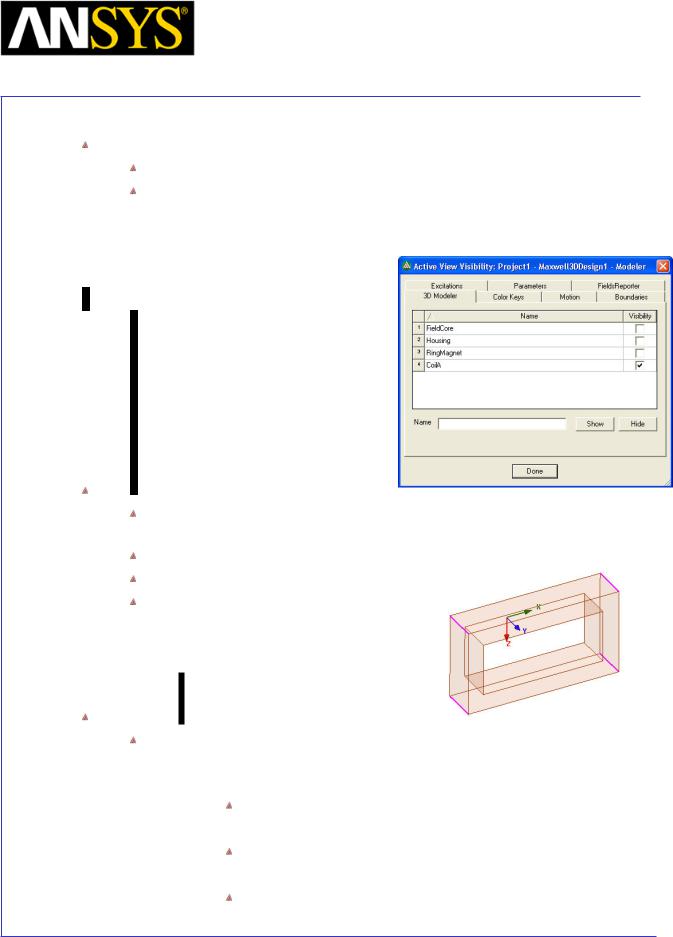
|
Maxwell v15 |
|
5.5 |
|
Example (Magnetostatic) |
– Anisotropic Material |
|
|
|
|
|
|
|
|
|
Hide All other Objects
Select the menu item View > Visibility > Active View Visibility
In Active View Visibility window
1.Change the visibility for all the objects to Unchecked
2.Keep the visibility for CoilA Checked
3.Press Done
Add Fillets
Select the menu item Edit > Select >Edges or press the key E from keyboard
Press Ctrl and select edges of coil as shown in image
Select the menu item Modeler > Fillet In Fillet Properties window,
1.Set Fillet Radius to 2
2.Press OK
Create Coordinate System to Split Coil
Select the menu item Modeler > Coordinate System > Create > Relative CS > Both
1. Using the coordinate entry fields, enter the origin
X: 0, Y: 0.2, Z: 0.2, Press the Enter key
2. Using the coordinate entry field, enter the X axis position
dX: 0, dY: 1, dZ: -1, Press the Enter key
3. Using the coordinate entry field, enter the XY Plane position dX: 0, dY: 1, dZ: 1, Press the Enter key
|
|
|
|
|
|
|
|
|
|
|
|
ANSYS Maxwell 3D Field Simulator v15 User’s Guide |
|
5.5-15 |
|||
|
|
|
|
|
|
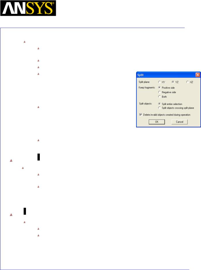
|
Maxwell v15 |
|
5.5 |
|
Example (Magnetostatic) |
– Anisotropic Material |
|
|
|
|
|
|
|
|
|
Split Coil
Select the menu item Edit > Select >Objects or press the key O from keyboard to change selection to Objects
Select the object CoilA from the tree
Select the menu item Modeler > Boolean > Split
In Split window,
1.Split Plane: YZ
2.Keep fragments: Positive side
3.Split Objects: Split entire selection
4.Press OK
Similarly perform Split with XZ Plane
1.Split Plane: XZ
2.Keep fragments: Positive side
3.Split Objects: Split entire selection
4.Press OK
Note: Ensure RelativeCS2 its work Coordinate system while performing
Split operation
Assign Material to Coil
To assign material:
Select the object Coil from the history tree, right click and select Assign Material
In Select Definition window,
1.Type copper in the Search by Name field
2.Click the OK button
Create Coil terminal
Change Work Coordinate System
Goto Modeler > Coordinate System > Set Working CS
In Select Coordinate System Window
1.Select Global
2.Press Select
|
|
|
|
|
|
|
|
|
|
|
|
ANSYS Maxwell 3D Field Simulator v15 User’s Guide |
|
5.5-16 |
|||
|
|
|
|
|
|
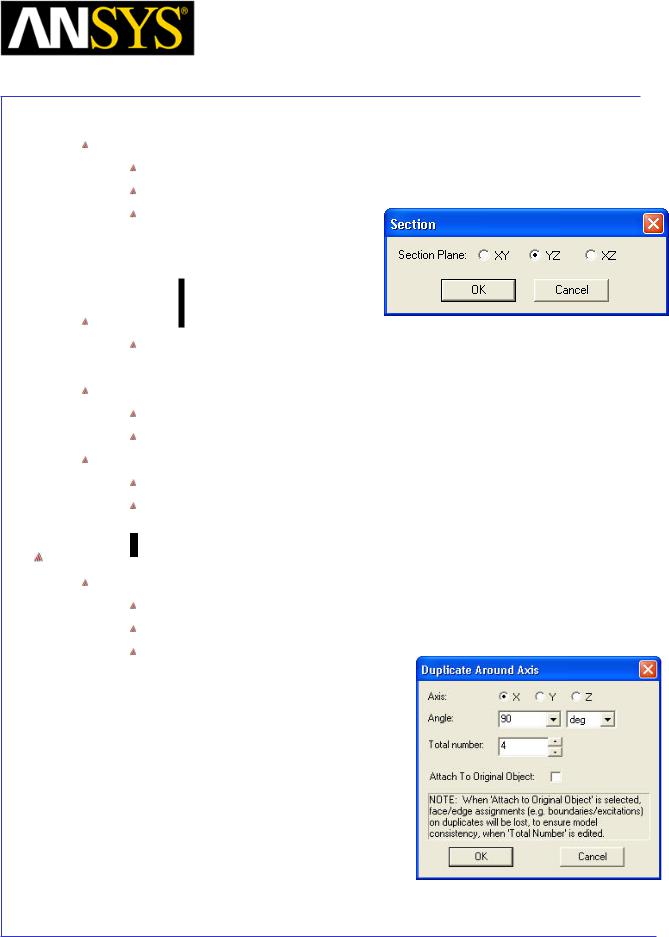
|
Maxwell v15 |
|
5.5 |
|
Example (Magnetostatic) |
– Anisotropic Material |
|
|
|
|
|
|
|
|
|
Create Coil Terminal
Select the object CoilA from the history tree
Select the menu item Modeler > Surface > Section
In Section window,
1.Section Plane: YZ
2.Click the OK button
Change Attributes
Select the object CoilA_Section1 from the tree and goto Properties window 1. Change the name of the object to Terminal_A
Separate Sheets
Select the sheet Terminal_A
Select the menu item Modeler > Boolean > Separate Bodies
Delete Extra Sheets
Select the sheet Terminal_A_Seperate1 from the tree Select the menu item Edit >Delete
Duplicate Coil and Terminal
To Duplicate Coil and Terminal
Press Ctrl and select the objects CoilA and Terminal_A
Select the menu item Edit > Duplicate > Around Axis
In Duplicate Around Axis window
1.Axis: X
2.Angle: 90
3.Total number : 4
4.Press OK
|
|
|
|
|
|
|
|
|
|
|
|
ANSYS Maxwell 3D Field Simulator v15 User’s Guide |
|
5.5-17 |
|||
|
|
|
|
|
|
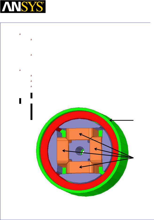
|
Maxwell v15 |
|
5.5 |
|
Example (Magnetostatic) |
– Anisotropic Material |
|
|
|
|
|
|
|
|
|
Change Attributes
Select the objects from the tree and goto Properties window
1.Change the name of the objects CoilA_2, CoilA_3 and CoilA_4 to CoilB, CoilC and CoilD
Select the sheets from the tree and goto Properties window,
1.Change the name of the sheets Terminal_A_1, Terminal_A_2 and Terminal_A_3 to Terminal_B, Terminal_C and Terminal_D
View all Objects
Select the menu item View > Visibility > Show All > Active View
Select Region from the history tree
Select the menu item View > Visibility > Hide Selection > Active View
Housing
FieldCore 
Coils
RingMagnet 
|
|
|
|
|
|
|
|
|
|
|
|
ANSYS Maxwell 3D Field Simulator v15 User’s Guide |
|
5.5-18 |
|||
|
|
|
|
|
|

|
Maxwell v15 |
|
5.5 |
|
Example (Magnetostatic) |
– Anisotropic Material |
|
|
|
|
|
|
|
|
|
Specify Excitations
Assign Excitations for CoilA and CoilC
Select the sheet Terminal_A and Terminal_C from the history tree
Select the menu item Maxwell 3D > Excitations > Assign > Current
In Current Excitation window,
1.Name: Current_A_C
2.Value: 4000
3.Type: Stranded
4.Current Direction: negative X (Use Swap Direction if needed)
5.Press OK
Assign Excitations for CoilB and CoilD
Select the sheet Terminal_B and Terminal_D from the history tree
Select the menu item Maxwell 3D > Excitations > Assign > Current
In Current Excitation window,
1.Name: Current_B_D
2.Value: 4000
3.Type: Stranded
4.Current Direction: positive X (Use Swap Direction if needed)
5.Press OK
Analysis Setup
To create an analysis setup:
Select the menu item Maxwell 3D > Analysis Setup > Add Solution Setup
Solution Setup Window:
1. General Tab
 Percentage Error: 5 2. Convergence Tab:
 Refinement Per Pass: 30 3. Solver Tab
 Nonlinear Residuals : 0.01 4. Click the OK button
|
|
|
|
|
|
|
|
|
|
|
|
|
|
|
|
|
|
|
|
|
|
|
|
|
|
|
|
|
|
|
|
|
|
|
|
|
|
|
|
|
|
|
|
|
|
|
|
|
|
ANSYS Maxwell 3D Field Simulator v15 User’s Guide |
|
5.5-19 |
|||||||
|
|
|
|
|
|
|
|
|
|
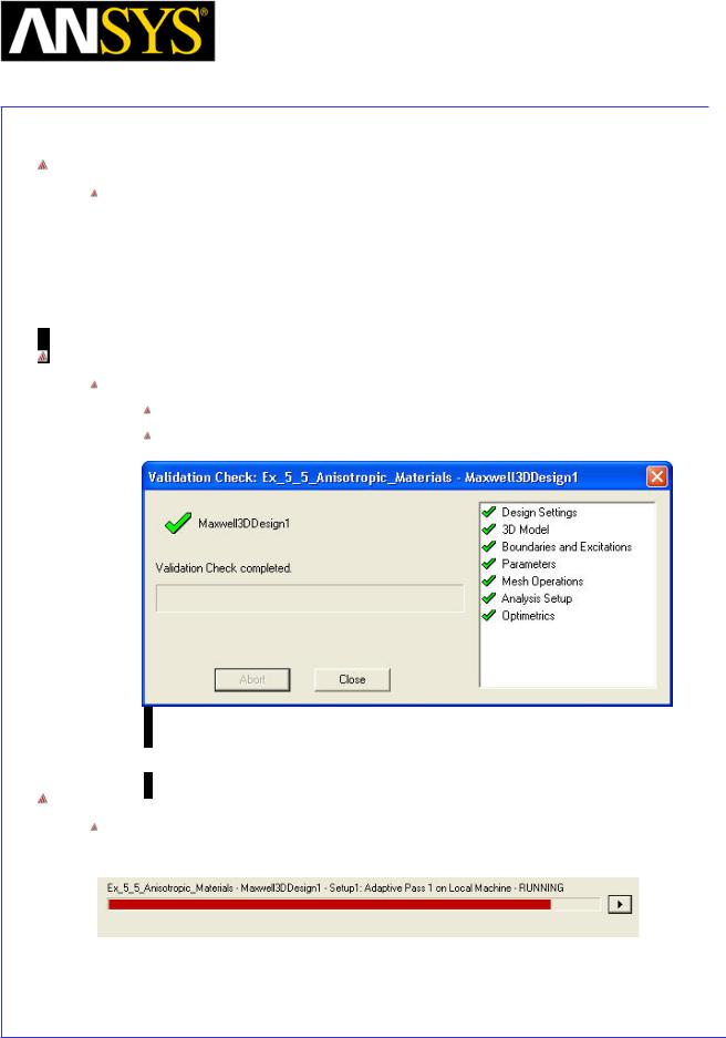
|
Maxwell v15 |
|
5.5 |
|
Example (Magnetostatic) |
– Anisotropic Material |
|
|
|
|
|
|
|
|
|
Save Project
To save the project:
1.In an Ansoft Maxwell window, select the menu item File > Save As.
2.From the Save As window, type the Filename: Ex_5_5_Anisotropic_Materials
3.Click the Save button
Model Validation
To validate the model:
Select the menu item Maxwell 3D > Validation Check
Click the Close button
Note: To view any errors or warning messages, use the Message Manager.
Analyze
To start the solution process:
1. Select the menu item Maxwell 3D > Analyze All
|
|
|
|
|
|
|
|
|
|
|
|
ANSYS Maxwell 3D Field Simulator v15 User’s Guide |
|
5.5-20 |
|||
|
|
|
|
|
|
|
Maxwell v15 |
|
5.5 |
|
Example (Magnetostatic) |
– Anisotropic Material |
|
|
|
|
|
|
|
|
|
Theory of the Nonlinear Anisotropic Material for soft magnetic materials
Basic ideas for new nonlinear anisotropic materials:
The cross effects of the magnetic field in the different principle directions are decoupled by introducing an equivalent magnetic field magnitude in each principle direction based on an anisotropic characterization of the energy density .
Only B-H curves in the principal directions of the materials – two curves in 2D or three curves in 3D – need to be measured
The anisotropic behavior of laminations with either isotropic or anisotropic steel is also considered.
Proposed approach
Since applying the same value of H in different principle directions will cause different level of magnetic saturations, the approach refers all components of H to each principle direction by referring factor k to determine the saturation in that direction
|
|
|
|
|
|
|
|
|
|
|
|
|
|
|
|
x |
|
2 |
|
|
|
2 |
|
2 |
|
|
|||
|
|
He |
= |
|
|
H x |
+(kxy H y ) |
|
+(kxz kµz H z ) |
|
|
|
||
|
|
|
|
|
||||||||||
|
|
|
|
|
|
|
|
|
|
|
|
|
|
|
|
y |
= |
|
|
(kyx H x ) |
2 |
+ H y |
2 |
+(kyz kµz H z ) |
2 |
|
|
||
|
|
He |
|
|
|
|
|
|
|
|||||
|
|
|
|
|
|
|
|
|
|
|
|
|
|
|
|
|
|
|
(kzx H x )2 +(kzy H y )2 +(kµz H z )2 |
||||||||||
|
Hez = |
|
||||||||||||
|
|
|
|
|
|
|
|
|
|
|
|
|
|
|
|
where |
|
is introduced to consider lamination effects and kxy is determined |
|||||||||||
by magnetic energy density w in x and y principle directions, kxy = wx /wy, and similarly to other k’s.
The permeability for each principle direction is obtained in terms of the equivalent magnitude He in that direction. For example, for axis x:
|
|
|
|
|
|
|
|
|
|
|
|
|
|
|
|
|
|
|
|
|
|
|
|
|
|
|
|
|
|
|
|
ANSYS Maxwell 3D Field Simulator v15 User’s Guide |
|
5.5-21 |
|||||
|
|
|
|
|
|
|
|
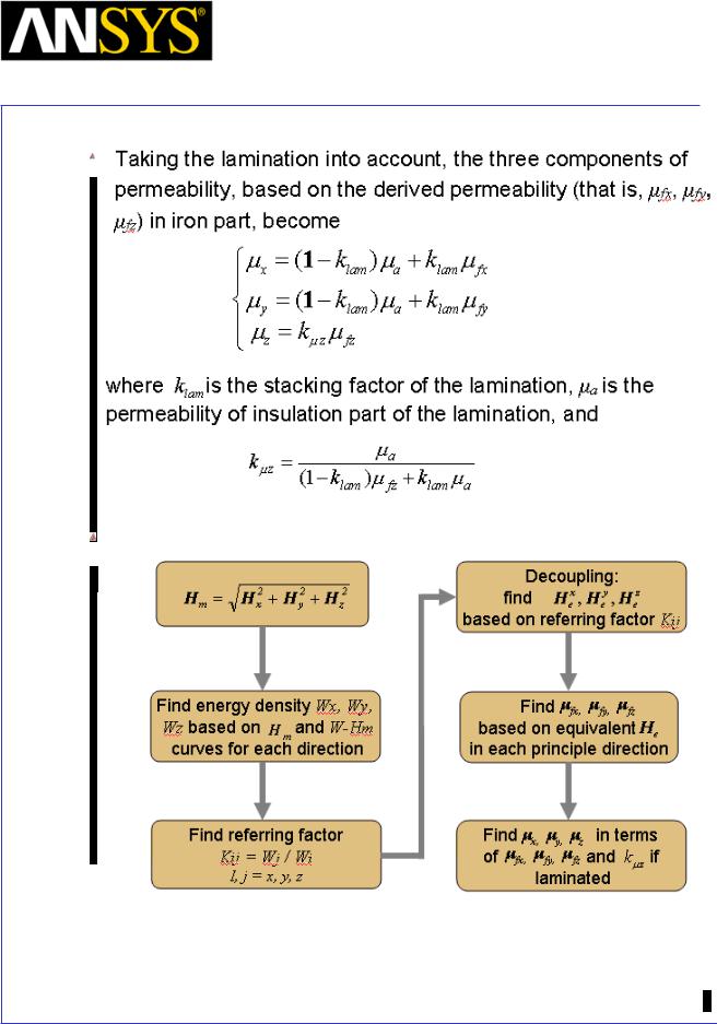
|
Maxwell v15 |
|
5.5 |
|
Example (Magnetostatic) |
– Anisotropic Material |
|
|
|
|
|
|
|
|
|
The Modeling Sequence will be as follows:
Reference:
[1] D. Lin, P. Zhou, Z. Badics, W. N. Fu, Q. M. Chen and Z. J. Cendes, “A New Nonlinear Anisotropic Model for Soft Magnetic Materials” , CSY0084 of COMPUMAG’2005
ANSYS Maxwell 3D Field Simulator v15 User’s Guide |
5.5-22 |
||
|
|
|
|
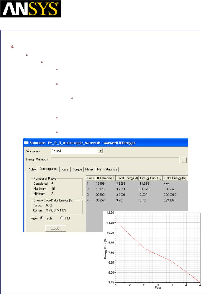
|
Maxwell v15 |
|
5.5 |
|
Example (Magnetostatic) |
– Anisotropic Material |
|
|
|
|
|
|
|
|
|
Solution Data
To view the Solution Data:
Select the menu item Maxwell 3D > Results > Solution Data
To view the Profile:
1. Click the Profile Tab. To view the Convergence:
1. Click the Convergence Tab
Note: The default view is for convergence is Table. Select the Plot radio button to view a graphical representations of the convergence data.
To View Mesh information
1. Click Mesh Statistics Tab Select Close to close the window
|
|
|
|
|
|
|
|
|
|
|
|
|
|
|
|
|
|
|
|
|
|
|
|
|
|
|
|
|
|
|
|
ANSYS Maxwell 3D Field Simulator v15 User’s Guide |
|
5.5-23 |
|||||
|
|
|
|
|
|
|
|
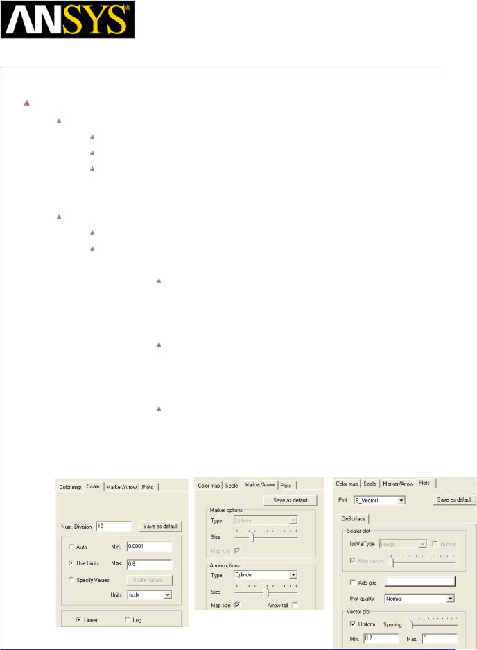
|
Maxwell v15 |
|
5.5 |
|
Example (Magnetostatic) |
– Anisotropic Material |
|
|
|
|
|
|
|
|
|
Vector Plot
Create Vector Plot
Select Global:YZ plane from history tree
Select menu item Maxwell 3D > Fields > Fields > B > B_Vector
In Create Field Plot window
1.In Volume: RingMagnet
2.Select Done
Modify Plot Attributes
Double click on the legend to change plot properties
In the window 1. Scale tab
User Limits: Checked
1.Min: 0.0001
2.Max: 0.8
2.Marker/Arrow tab
Arrow Options
1.Size: Six spaces from left
2.Arrow tail: Unchecked
3. Plots tab
Vector Plot
1.Spacing: Set to Minimum
2.Min: 0.7
3.Max: 3
4.Press Apply and Close
|
|
|
|
|
|
|
|
|
|
|
|
ANSYS Maxwell 3D Field Simulator v15 User’s Guide |
|
5.5-24 |
|||
|
|
|
|
|
|
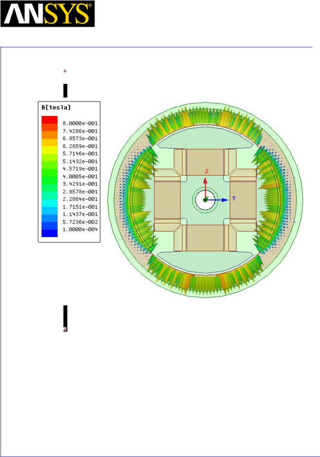
|
Maxwell v15 |
|
5.5 |
|
Example (Magnetostatic) |
– Anisotropic Material |
|
|
|
|
|
|
|
|
|
The plot of the flux density on YZ cut plane of the Mag will be as below:
Note: Please note that if the RingMagnet is not set up as anisotropic one (i.e. uniform Nonlinear one) the B field between two magnetic poles will be very large in the theta directions, which will be not as good as user wanted.
|
|
|
|
|
|
|
|
|
|
|
|
ANSYS Maxwell 3D Field Simulator v15 User’s Guide |
|
5.5-25 |
|||
|
|
|
|
|
|
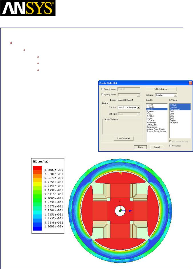
|
Maxwell v15 |
|
5.5 |
|
Example (Magnetostatic) |
– Anisotropic Material |
|
|
|
|
|
|
|
|
|
Plot Flux Density Contours
To Plot contours of Magnetic Flux Density
Select Global:YZ plane from history tree
Select menu item Maxwell 3D > Fields > Fields > B > Mag_B
In Create Field Plot window
1.In Volume: Press Ctrl and select objects FieldCore, Housing and RingMagnet
2.Select Done
|
|
|
|
|
|
|
|
|
|
|
|
|
|
|
|
|
|
|
|
|
|
|
|
|
|
|
|
|
|
|
|
ANSYS Maxwell 3D Field Simulator v15 User’s Guide |
|
5.5-26 |
|||||
|
|
|
|
|
|
|
|

|
Maxwell v15 |
|
5.5 |
|
Example (Magnetostatic) |
– Anisotropic Material |
|
|
|
|
|
|
|
|
|
Create Rectangular Plot
Create Arc for Rectangular plot
Select menu item Draw > Arc > 3 Point
A massage will pop up asking if the entity needs to be created as non model object. Select Yes to it.
1. Using Co-ordinate entry field Enter the first end point
X = 0, Y = 13.435, Z = 13.435, Press Enter
2. Using Co-ordinate entry field Enter the arc intercept (middle point)
X = 0, Y = 0, Z = 19, Press Enter
3. Using Co-ordinate entry field Enter the second end point
 X = 0, Y = -13.435, Z = 13.435, Press Enter 4. Press Enter to exit
Create parameter for radial magnetic filed strength Goto Maxwell 3D > Fileds > Calculator
1.Select Input > Quantity > B
2.Select General > Smooth
3.Select Vector > Scal? > ScalarX
4.Select Input > Function > Scalar > PHI
5.Select Scalar > Trig > Cos
6.Select General > *
7.Select Input > Quantity > B
8.Select General > Smooth
9.Select Vector > Scal? > ScalarY
10.Select Input > Function > Scalar > PHI
11.Select Scalar > Trig > Sin
12.Select General > *
13.Select General > +
14.Select Add and set the name of expression as Brad
15.Press Done
|
|
|
|
|
|
|
|
|
|
|
|
|
|
|
|
|
|
|
|
|
|
|
|
|
|
|
|
|
|
|
|
ANSYS Maxwell 3D Field Simulator v15 User’s Guide |
|
5.5-27 |
|||||
|
|
|
|
|
|
|
|
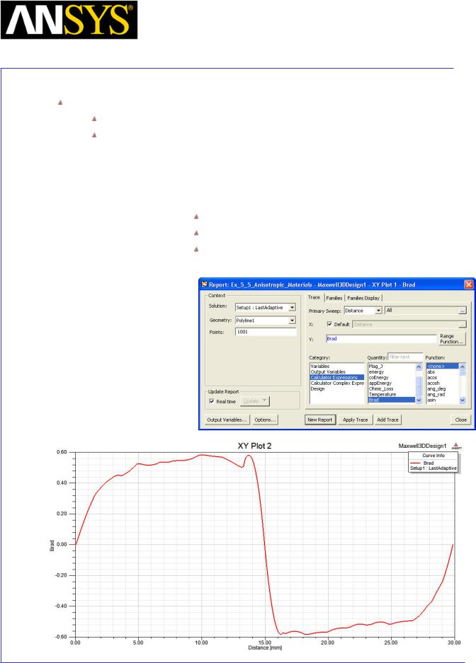
|
Maxwell v15 |
|
5.5 |
|
Example (Magnetostatic) |
– Anisotropic Material |
|
|
|
|
|
|
|
|
|
To Create Plot:
Select Maxwell 3D > Results > Create Fields Report > Rectangular Plot
In Reports window
1.Geometry: Polyline1
2.Trace Tab
1.X axis: Default
2.Y axis
Category: Calculator Expressions
Quantity: Brad
Function: None
3. Select New Report
|
|
|
|
|
|
|
|
|
|
|
|
|
|
|
|
|
|
|
|
|
|
|
|
|
|
|
|
|
|
|
|
ANSYS Maxwell 3D Field Simulator v15 User’s Guide |
|
5.5-28 |
|||||
|
|
|
|
|
|
|
|
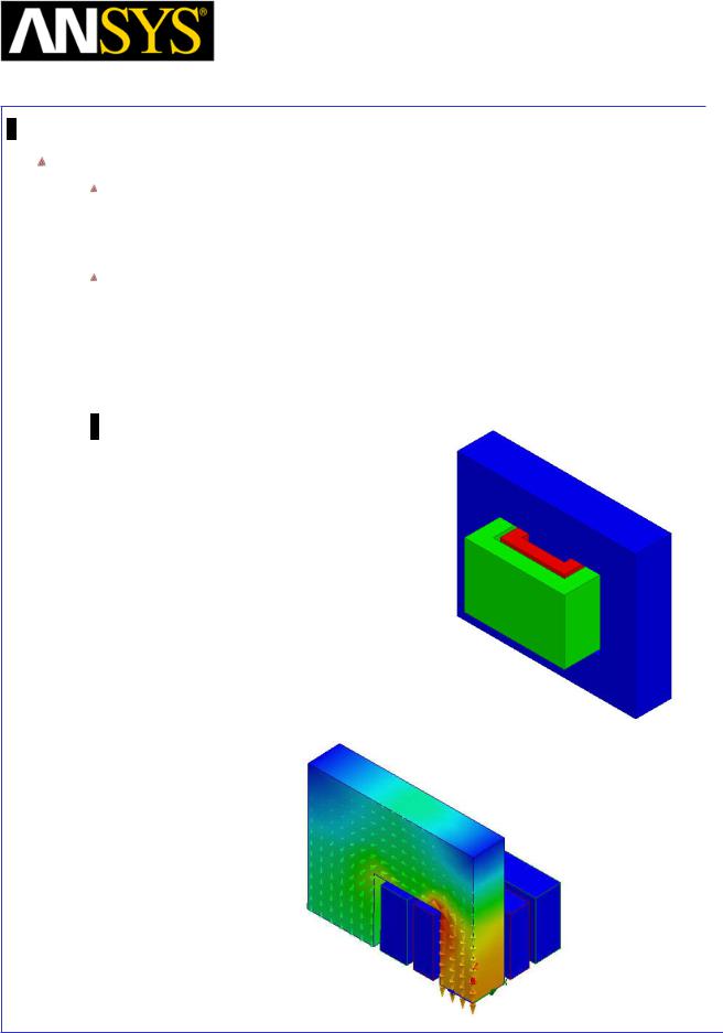
Maxwell v15 |
5.6 |
Example (Magnetostatic) – Symmetry Boundaries
The application of Symmetry Boundaries
There are many advantages to using Symmetry Boundaries when modeling.
Meshes can be decreased greatly by using Symmetry Boundaries when you model the shape of an analytical object . As a result, the saving of the calculation resource and shortening analytical time become possible.
In this note, the model of very simple transformer will be analyzed using
Magnetostatic solver. At this time, the model size is reduced by using the
Symmetry boundaries. The intent of this write up is not how to simulate the Transformer, it is rather to demonstrate how Symmetry boundaries is implemented within the Magnetostatic solver. A very simple transformer that rolls the winding of Coil_In and Coil_Out in core is used.
Complete Geometry
Symmetry Model
|
|
|
|
|
|
|
|
|
|
|
|
ANSYS Maxwell 3D Field Simulator v15 User’s Guide |
|
5.6-1 |
|||
|
|
|
|
|
|

Maxwell v15 |
5.6 |
Example (Magnetostatic) – Symmetry Boundaries
ANSYS Maxwell Design Environment
The following features of the ANSYS Maxwell Design Environment are used to
create the models covered in this topic
3D Solid Modeling
Primitives: Line, Rectangle, Box
Surface Operations: Section, Sweep Along Path
Boolean Operations: Subtract, Separate Bodies, Split,
Duplicate (Mirror)
Boundaries/Excitations
Current: Stranded
Symmetry
Analysis
Magnetostatic
Results
Solution Data
Field Overlays:
Flux Density Plots
|
|
|
|
|
|
|
|
|
|
|
|
|
|
|
|
|
|
|
|
|
|
|
|
|
|
|
|
|
|
|
|
|
|
|
|
|
|
|
|
|
|
|
|
|
|
|
|
|
|
|
|
|
|
|
|
|
|
|
|
ANSYS Maxwell 3D Field Simulator v15 User’s Guide |
|
5.6-2 |
|||||||
|
|
|
|
|
|
|
|
|
|
Maxwell v15 |
5.6 |
Example (Magnetostatic) – Symmetry Boundaries
Launching Maxwell
To access Maxwell:
1.Click the Microsoft Start button, select Programs, and select Ansoft > Maxwell 15.0 and select Maxwell 15.0
Setting Tool Options
To set the tool options:
Note: In order to follow the steps outlined in this example, verify that the following tool options are set :
1. Select the menu item Tools > Options > Maxwell 3D Options
Maxwell Options Window:
1. Click the General Options tab
Use Wizards for data input when creating new boundaries: Checked
Duplicate boundaries/mesh operations with geometry:
Checked
2.Click the OK button
2.Select the menu item Tools > Options > Modeler Options.
Modeler Options Window:
1. Click the Operation tab
 Automatically cover closed polylines: Checked 2. Click the Display tab
 Default transparency = 0.8 3. Click the Drawing tab
 Edit property of new primitives: Checked 4. Click the OK button
|
|
|
|
|
|
|
|
|
|
|
|
|
|
|
|
|
|
|
|
|
|
|
|
|
|
|
|
|
|
|
|
ANSYS Maxwell 3D Field Simulator v15 User’s Guide |
|
5.6-3 |
|||||
|
|
|
|
|
|
|
|
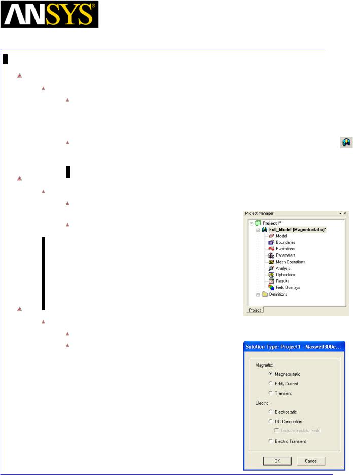
Maxwell v15 |
5.6 |
Example (Magnetostatic) – Symmetry Boundaries
Opening a New Project
To open a new project:
After launching Maxwell, a project will be automatically created. You can also create a new project using below options.
1.In an Maxwell window, click the On the Standard toolbar, or select the menu item File > New.
Select the menu item Project > Insert Maxwell 3D Design, or click on the icon
Change Design name
To Change Design Name:
Right-click Maxwell3D Design1 at the project manager window and select Rename.
Change the Design Name to Full_Model
Set Solution Type
To set the Solution Type:
Select the menu item Maxwell 3D > Solution Type
Solution Type Window:
1.Choose Magnetostatic
2.Click the OK button
|
|
|
|
|
|
|
|
|
|
|
|
|
|
|
|
|
|
|
|
|
|
|
|
|
|
|
|
|
|
|
|
|
|
|
|
|
|
|
|
|
|
|
|
|
|
|
|
|
|
ANSYS Maxwell 3D Field Simulator v15 User’s Guide |
|
5.6-4 |
|||||||
|
|
|
|
|
|
|
|
|
|
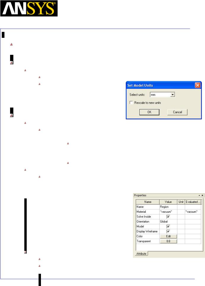
Maxwell v15 |
5.6 |
Example (Magnetostatic) – Symmetry Boundaries
Example 1: Solve Full Model
Set Model Units
To Set the units:
Select the menu item Modeler > Units
Set Model Units:
1.Select Units: mm
2.Click the OK button
Create Region
Create a Box region
Select the menu item Draw > Box or click on the icon.
icon.
1. Using the coordinate entry field, enter the box position X: -75, Y: -75, Z: -75 Press the Enter key
2.Using the coordinate entry fields, enter the opposite corner of the box:
dX: 150, dY: 150, dZ: 150, Press the Enter key
Change Attributes
Select the resulting object from the tree and goto Properties window
1.Change the name of the object to Region
2.Display Wireframe: Checked
Hide Region
Select Region from the history tree
Select the menu item View > Visibility > Hide Selection > Active View
|
|
|
|
|
|
|
|
|
|
|
|
ANSYS Maxwell 3D Field Simulator v15 User’s Guide |
|
5.6-5 |
|||
|
|
|
|
|
|
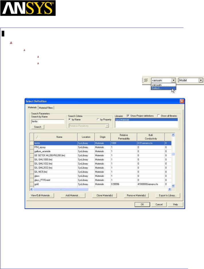
Maxwell v15 |
5.6 |
Example (Magnetostatic) – Symmetry Boundaries
Set Default Material
To set the default material:
Using the 3D Modeler Materials toolbar, choose Select
In Select Definition window,
1.Type ferrite in the Search by Name field
2.Click the OK button
|
|
|
|
|
|
|
|
|
|
|
|
|
|
|
|
|
|
|
|
|
|
|
|
|
|
|
|
|
|
|
|
ANSYS Maxwell 3D Field Simulator v15 User’s Guide |
|
5.6-6 |
|||||
|
|
|
|
|
|
|
|
Maxwell v15 |
5.6 |
Example (Magnetostatic) – Symmetry Boundaries
Create Core
Change Grid Plane
Select the menu item Modeler > Grid Plane > YZ
Create Rectangle
Select menu item Draw > Rectangle.
1. Using the coordinate entry fields, enter the rectangle position X: 5, Y: -25, Z: -20, Press the Enter key
2.Using the coordinate entry fields, enter the opposite corner of the rectangle
dX: 0, dY: 50, dZ: 40, Press the Enter key
Select the resulting object from the tree and goto Properties window
1.Change the name of the object to Core
2.Change the color of the object to Blue
Create Slot
Select menu item Draw > Rectangle.
1. Using the coordinate entry fields, enter the rectangle position X: 5, Y: -15, Z: 10, Press the Enter key
2.Using the coordinate entry fields, enter the opposite corner of the rectangle
dX: 0, dY: 10, dZ: -20, Press the Enter key
Select the resulting object from the tree and goto Properties window 1. Change the name of the object to Slot
Duplicate Slot
Select the object Slot from the history tree Select the menu item Edit > Duplicate > Mirror
1.Using the coordinate entry field, enter the anchor point of mirror plane
X: 0, Y: 0, Z: 0, Press the Enter key
2.Using the coordinate entry field, enter the target point of vector normal to the mirror plane
dX: 0, dY: 1, dZ: 0, Press the Enter key
|
|
|
|
|
|
|
|
|
|
|
|
|
|
|
|
|
|
|
|
|
|
|
|
|
|
|
|
|
|
|
|
|
|
|
|
ANSYS Maxwell |
3D Field Simulator v15 User’s Guide |
|
|
5.6-7 |
||||
|
|
|
|
|
|
|
|
|
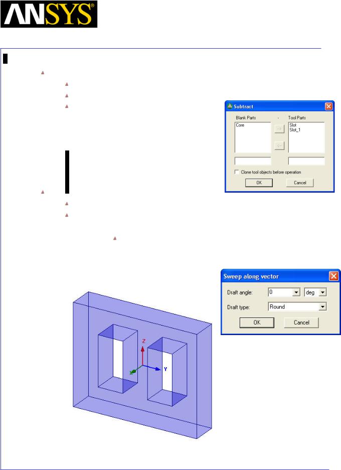
Maxwell v15 |
5.6 |
Example (Magnetostatic) – Symmetry Boundaries
Subtract Slot from Core
Press Ctrl and select the objects Core, Slot and Slot_1
Select the menu item Modeler > Boolean > Subtract
In Subtract Window,
1.Blank Parts: Core
2.Tool Parts: Slot, Slot_1
3.Click the OK button
Sweep Object
Select the object Core from the history tree
Select the menu item Draw > Sweep >Along Vector
1. Using the coordinate entry field, enter the first point of the vector
X: 0, Y: 0, Z:0, Press the Enter key
2. Using the coordinate entry field, enter the last point of the vector  dX: -10, dY: 0, dZ:0, Press the Enter key
3. Press OK
|
|
|
|
|
|
|
|
|
|
|
|
|
|
|
|
|
|
|
|
|
|
|
|
|
|
|
|
|
|
|
|
|
|
|
|
|
|
|
|
|
|
|
|
|
|
|
|
|
|
ANSYS Maxwell 3D Field Simulator v15 User’s Guide |
|
5.6-8 |
|||||||
|
|
|
|
|
|
|
|
|
|
Maxwell v15 |
5.6 |
Example (Magnetostatic) – Symmetry Boundaries
Set Default Material
To set the default material:
Using the 3D Modeler Materials toolbar, choose Select
In Select Definition window,
1.Type copper in the Search by Name field
2.Click the OK button
Create Coil_In
Create Box
Select the menu item Draw > Box
1. Using the coordinate entry fields, enter the box position
X: -9, Y: -9, Z: -9, Press the Enter key
2. Using the coordinate entry fields, enter opposite corner of the box:
dX: 18, dY: 18, dZ: 18, Press the Enter key
Change Attributes
Select the resulting object from the tree and goto Properties window
1.Change the name of the object to Coil_In
2.Change its color to Red
Create another Box
Select the menu item Draw > Box
1. Using the coordinate entry fields, enter the box position
X: -6, Y: -6, Z: -9, Press the Enter key
2. Using the coordinate entry fields, enter opposite corner of the box:
 dX: 12, dY: 12, dZ: 18, Press the Enter key Change Attributes
Select the resulting object from the tree and goto Properties window 1. Change the name of the object to Coil_In_1
Subtract Objects
Press Ctrl and select the objects Coil_In and Coil_In_1
Select the menu item Modeler > Boolean > Subtract
In Subtract Window,
1.Blank Parts: Coil_In
2.Tool Parts: Coil_In_1
3.Click the OK button
|
|
|
|
|
|
|
|
|
|
|
|
|
|
ANSYS |
Maxwell 3D Field Simulator v15 User’s Guide |
|
5.6-9 |
|||
|
|
|
|
|
|
|

Maxwell v15 |
5.6 |
Example (Magnetostatic) – Symmetry Boundaries
Create Coil_Out
Create Profile for Sweep
Select menu item Draw > Rectangle.
1. Using the coordinate entry fields, enter the rectangle position X: 0, Y: 10, Z: -9, Press the Enter key
2.Using the coordinate entry fields, enter the opposite corner of the rectangle
dX: 0, dY: 4, dZ: 18, Press the Enter key
Select the resulting object from the tree and goto Properties window
1.Change the name of the object to Coil_Out
2.Change the color of the object to Green
Create Path for Sweep
Select the menu item Draw > Line
1. Using the coordinate entry field, enter the first point of the line
X: 10, Y: 10, Z: 9, Press the Enter key
2. Using the coordinate entry field, enter the second point of the line
X: -10, Y: 10, Z: 9, Press the Enter key
3. Using the coordinate entry field, enter the next point of the line
X: -10, Y: -10, Z: 9, Press the Enter key
4. Using the coordinate entry field, enter the next point of the line
X: 10, Y: -10, Z: 9, Press the Enter key
5. Using the coordinate entry field, enter the first point of the line
 X: 10, Y: 10, Z: 9, Press the Enter key 6. Press Enter
Select the resulting object from the tree and goto Properties window 1. Change the name of the object to Coil_Out_Path
Select the object Coil_Out_Path and select the menu item Modeler > Delete Last Operation
Note: The object created in the last step results into a sheet. In order to get a polyline, we delete the Coverlines command that is automatically performed.
|
|
|
|
|
|
|
|
|
|
|
|
ANSYS Maxwell 3D Field Simulator v15 User’s Guide |
|
5.6-10 |
|||
|
|
|
|
|
|
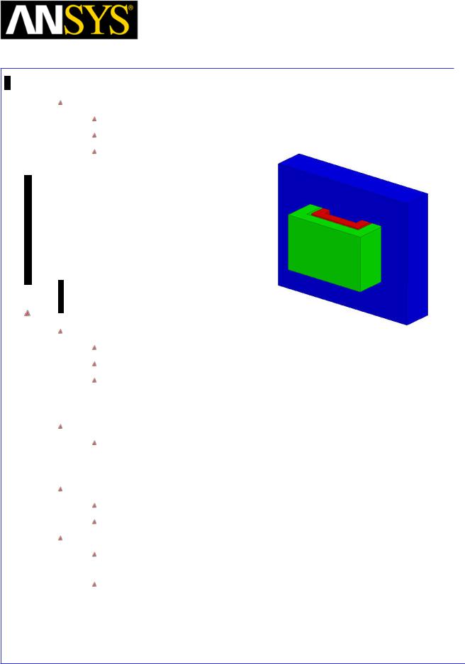
Maxwell v15 |
5.6 |
Example (Magnetostatic) – Symmetry Boundaries
Create Sweep
Press Ctrl and select the objects Coil_Out and Coil_Out_Path from the tree
Select the menu item Draw > Sweep >Along Path
Press OK
Create Coil Terminals
Create Section
Press Ctrl and select the objects Coil_In and Coil_Out from the tree
Select the menu item Modeler > Surface >Section
In Section window,
1.Section Plane: YZ
2.Click the OK button
Change Attributes
Select the object Coil_In_Section1 and Coil_Out_Section1 from the tree and goto Properties window
1. Change the name of the object to Term_In and Term_Out Separate Sections
Press Ctrl and select the objects Term_In and Term_Out from the tree
Select the menu item Modeler > Boolean > Separate Bodies
Delete Extra Sheets
Press Ctrl and select the object Term_In_Separate1 and Term_Out_Separate1 from the tree
Select the menu item Edit > Delete
|
|
|
|
|
|
|
|
|
|
|
|
|
|
|
|
|
|
|
|
|
|
|
|
|
|
|
|
|
|
|
|
|
|
|
|
|
|
|
|
|
|
|
|
|
|
|
|
|
|
|
|
|
|
|
|
|
|
|
|
|
|
Maxwell 3D Field Simulator v15 User’s Guide |
|
5.6-11 |
|||||
ANSYS |
|
|
|||||||
|
|
|
|
|
|
|
|
|
|
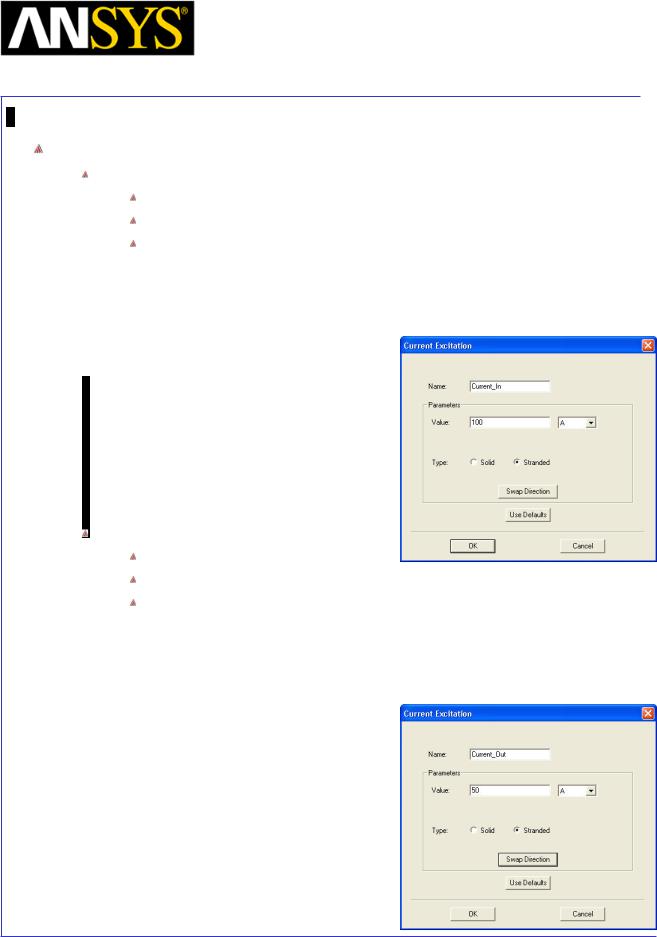
Maxwell v15 |
5.6 |
Example (Magnetostatic) – Symmetry Boundaries
Create Excitations
Assign Excitation for Coil_In
Select the object Term_In
Select the menu item Maxwell 3D > Excitations > Assign >Current
In Current Excitation window,
1.Name: Current_In
2.Value: 100 A
3.Type: Stranded
4.Direction: Positive X (Use Swap Direction if needed)
5.Press OK
Assign Excitation for Coil_Out
Select the object Term_Out
Select the menu item Maxwell 3D > Excitations > Assign >Current
In Current Excitation window,
1.Name: Current_Out
2.Value: 50 A
3.Type: Stranded
4.Direction: Negative X (Use Swap Direction if needed)
5.Press OK
|
|
|
|
|
|
|
|
|
|
|
|
|
|
|
|
|
|
|
|
|
|
|
|
|
|
|
|
|
|
|
|
ANSYS Maxwell 3D Field Simulator v15 User’s Guide |
|
5.6-12 |
|||||
|
|
|
|
|
|
|
|
Maxwell v15 |
5.6 |
Example (Magnetostatic) – Symmetry Boundaries
Analysis Setup
To create an analysis setup:
Select the menu item Maxwell 3D > Analysis Setup > Add Solution Setup
Solution Setup Window:
1. Click the OK button to accept all default settings.
Save Project
To save the project:
1.In an Ansoft Maxwell window, select the menu item File > Save As.
2.From Save As window, type the Filename: Ex_5_6_Symmetry_Boundaries
3.Click the Save button
Model Validation
To validate the model:
Select the menu item Maxwell 3D > Validation Check
Click the Close button
Note: To view any errors or warning messages, use the Message Manager.
Analyze
To start the solution process:
1. Select the menu item Maxwell 3D > Analyze All
|
|
|
|
|
|
|
|
|
|
|
|
|
|
|
|
|
|
|
|
|
|
|
|
|
|
|
|
|
|
|
|
ANSYS Maxwell 3D Field Simulator v15 User’s Guide |
|
5.6-13 |
|||||
|
|
|
|
|
|
|
|
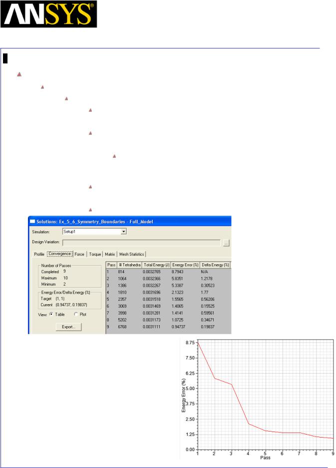
Maxwell v15 |
5.6 |
Example (Magnetostatic) – Symmetry Boundaries
Solution Data
To view the Solution Data:
Select the menu item Maxwell 3D > Results > Solution Data
To view the Profile:
1. Click the Profile Tab. To view the Convergence:
1. Click the Convergence Tab
Note: The default view is for convergence is Table. Select the Plot radio button to view a graphical representations of the convergence data.
To View Mesh information
1. Click Mesh Statistics Tab Select Close to close the window
|
|
|
|
|
|
|
|
|
|
|
|
|
|
|
|
|
|
|
|
|
|
|
|
|
|
|
|
|
|
|
|
ANSYS Maxwell 3D Field Simulator v15 User’s Guide |
|
5.6-14 |
|||||
|
|
|
|
|
|
|
|
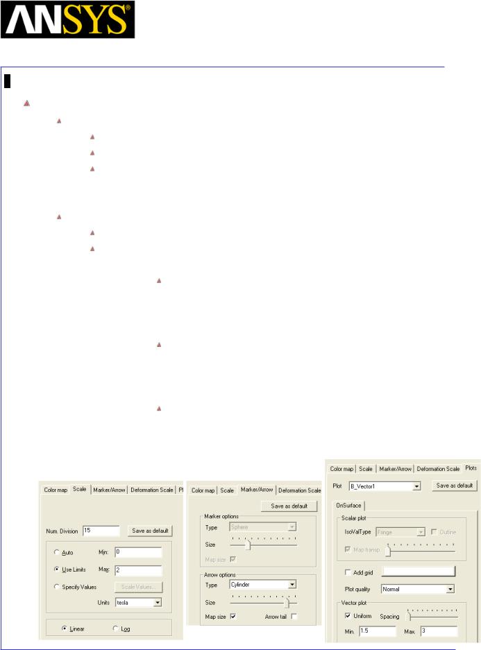
Maxwell v15 |
5.6 |
Example (Magnetostatic) – Symmetry Boundaries
Vector Plot
Create Vector Plot
Select Global:YZ plane from history tree
Select menu item Maxwell 3D > Fields > Fields > B > B_Vector
In Create Field Plot window
1.In Volume: AllObjects
2.Select Done
Modify Plot Attributes
Double click on the legend to change plot properties
In the window 1. Scale tab
User Limits: Checked
1.Min: 0
2.Max: 2
2.Marker/Arrow tab
Arrow Options
1.Size: Set to appropriate value
2.Arrow tail: Unchecked
3. Plots tab
Vector Plot
1.Spacing: Set to Minimum
2.Min: 1.5
3.Max: 3
4.Press Apply and Close
|
|
|
|
|
|
|
|
|
|
|
|
ANSYS Maxwell 3D Field Simulator v15 User’s Guide |
|
5.6-15 |
|||
|
|
|
|
|
|
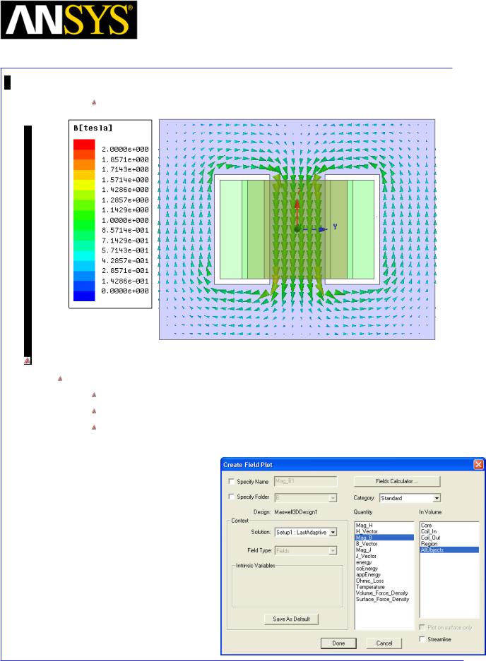
Maxwell v15 |
5.6 |
Example (Magnetostatic) – Symmetry Boundaries
The plot of the flux density on YZ plane will be as below:
Plot Flux Density Contours
To Plot contours of Magnetic Flux Density
Select Global:YZ plane from history tree
Select menu item Maxwell 3D > Fields > Fields > B > Mag_B
In Create Field Plot window
1.In Volume: AllObjects
2.Select Done
|
|
|
|
|
|
|
|
|
|
|
|
ANSYS Maxwell 3D Field Simulator v15 User’s Guide |
|
5.6-16 |
|||
|
|
|
|
|
|
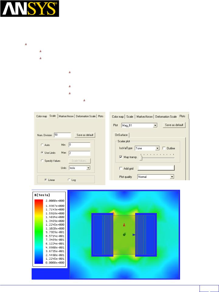
|
|
|
Maxwell v15 |
5.6 |
|||
|
|
Example (Magnetostatic) – Symmetry Boundaries |
|||||
|
|
|
|
|
|
|
|
|
|
Modify Plot Attributes |
|
|
|
|
|
|
|
|
|
|
|
||
|
|
|
|
|
|
||
|
|
Double click on the legend to change plot properties |
|
|
|
|
|
|
|
In the window |
|
|
|
|
|
1. |
Scale tab |
|
|
|
|
||
|
|
|
Num. Divisions: 50 |
|
|
|
|
2. |
Plots tab |
|
|
|
|
||
|
|
|
Plot: Mag_B1 |
|
|
|
|
|
|
|
Scalar Plot |
|
|
|
|
|
|
|
IsoValType: Tone |
|
|
|
|
3. |
Press Apply and Close |
|
|
|
|
||
|
|
|
|
|
|
|
|
|
|
|
|
|
|
|
|
|
|
|
|
|
|
|
|
ANSYS Maxwell 3D Field Simulator v15 User’s Guide |
5.6-17 |
||
|
|
|
|
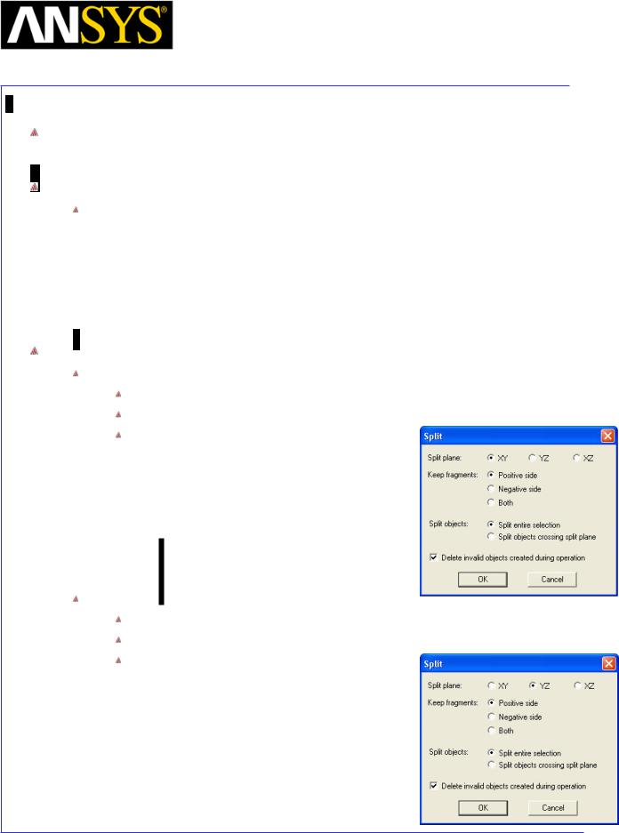
Maxwell v15 |
5.6 |
Example (Magnetostatic) – Symmetry Boundaries
Example 2: Solve 1/8th of Model using Symmetry
Create Symmetry Design
Copy Design
1.Select the design Full_Model in Project Manager window, right click and select Copy
2.Select project Ex_5_6_Symmetry_Boundaries in Project Manager window and select Paste
3.Change the name of the design to 1_8_Model
Split Model for 1/8th Section
Divide by XY Plane
Select the menu item Edit > Select All
Select the menu item Modeler > Boolean >Split
In Split window
1.Split plane: XY
2.Keep fragments: Positive side
3.Split objects: Split entire selection
4.Press OK
Divide by YZ Plane
Select the menu item Edit > Select All
Select the menu item Modeler > Boolean >Split
In Split window
1.Split plane: YZ
2.Keep fragments: Positive side
3.Split objects: Split entire selection
4.Press OK
|
|
|
|
|
|
|
|
|
|
|
|
|
|
|
|
|
|
|
|
|
|
|
|
|
|
|
|
|
|
|
|
ANSYS Maxwell 3D Field Simulator v15 User’s Guide |
|
5.6-18 |
|||||
|
|
|
|
|
|
|
|
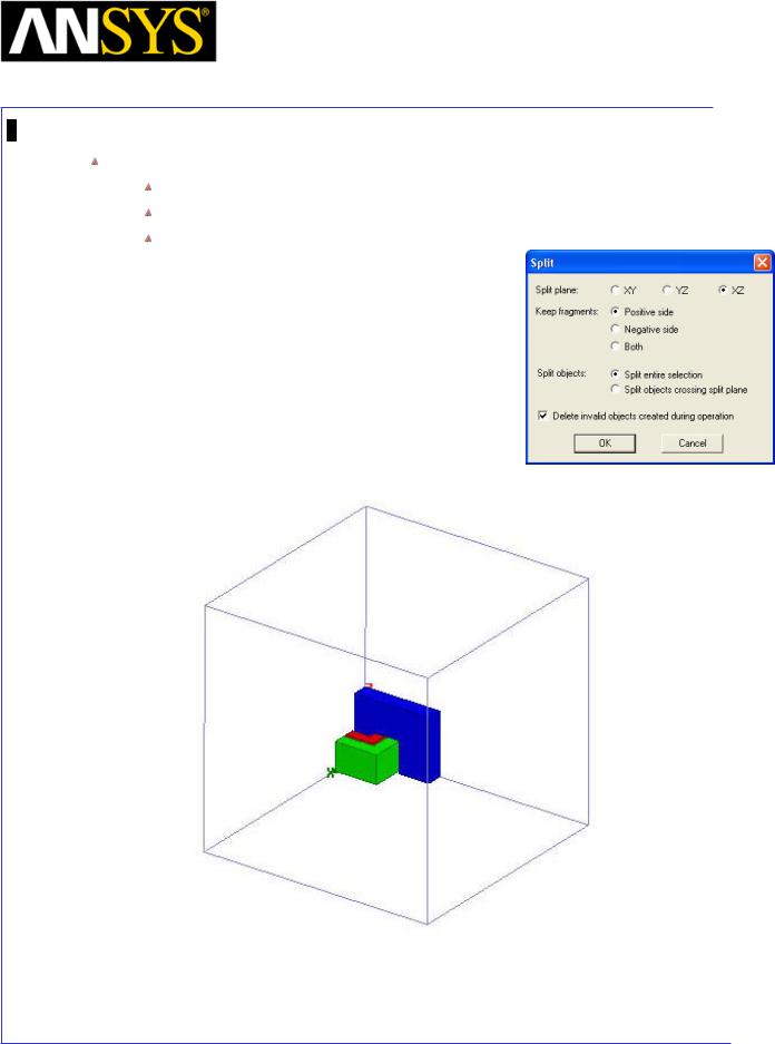
Maxwell v15 |
5.6 |
Example (Magnetostatic) – Symmetry Boundaries
Divide by XZ Plane
Select the menu item Edit > Select All
Select the menu item Modeler > Boolean >Split
In Split window
1.Split plane: XZ
2.Keep fragments: Positive side
3.Split objects: Split entire selection
4.Press OK
|
|
|
|
|
|
|
|
|
|
|
|
|
|
|
|
|
|
|
|
|
|
|
|
|
|
|
|
|
|
|
|
ANSYS Maxwell 3D Field Simulator v15 User’s Guide |
|
5.6-19 |
|||||
|
|
|
|
|
|
|
|
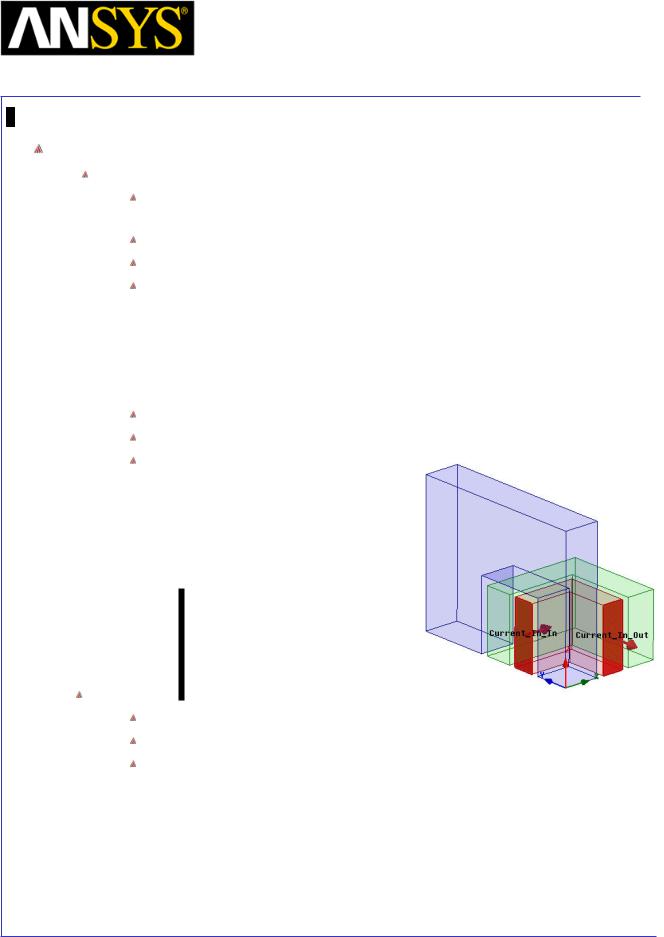
Maxwell v15 |
5.6 |
Example (Magnetostatic) – Symmetry Boundaries
Create Excitations
Assign Excitation for Coil_In
Select the menu item Edit > Select > Faces or press F from the keyboard to change selection to faces
Select the face of Coil_In which touches the YZ Plane
Select the menu item Maxwell 3D > Excitations > Assign >Current
In Current Excitation window,
1.Name: Current_In_In
2.Value: 50 A
3.Type: Stranded
4.Direction: Positive X
5.Press OK
Select the face of Coil_In which touches the XZ Plane
Select the menu item Maxwell 3D > Excitations > Assign >Current
In Current Excitation window,
1.Name: Current_In_Out
2.Value: 50 A
3.Type: Stranded
4.Direction: Negative Y
5.Press OK
Assign Excitation for Coil_Out
Select the face of Coil_Out which touches the YZ Plane
Select the menu item Maxwell 3D > Excitations > Assign >Current
In Current Excitation window,
1.Name: Current_Out_Out
2.Value: 25 A
3.Type: Stranded
4.Direction: Negative X
5.Press OK
|
|
|
|
|
|
|
|
|
|
|
|
|
|
|
|
|
|
|
|
|
|
|
|
|
|
|
|
|
|
|
|
ANSYS Maxwell 3D Field Simulator v15 User’s Guide |
|
5.6-20 |
|||||
|
|
|
|
|
|
|
|
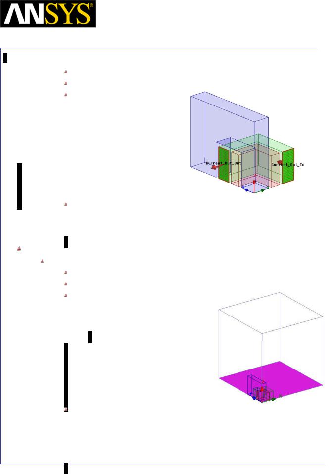
Maxwell v15 |
5.6 |
Example (Magnetostatic) – Symmetry Boundaries
Select the face of Coil_Out which touches the XZ Plane
Select the menu item Maxwell 3D > Excitations > Assign >Current
In Current Excitation window,
1.Name: Current_Out_In
2.Value: 25 A
3.Type: Stranded
4.Direction: Positive Y
5.Press OK
Note: The current value of Coil_In was 100A and Coil_Out was 50A in full model. The sectional area of the coil is 1/2 in 1/8 models because it is divided by XY plane. Therefore, the current value becomes 1/2, too.
Assign Boundaries
To Assign Symmetry Boundaries
Select the face of the Region with which touch with XY Plane
Select the menu item Maxwell 3D > Boundaries > Assign > Symmetry
In Symmetry Boundary window,
1.Symmetry: Even (Flux Normal)
2.Press OK
Note: The surface of boundary area (region) is analyzed as a natural boundary condition (Flux is the horizontal compared with respect). Because Flux becomes the horizontal for the YZ plane and the XZ plane in this model, the Symmetry boundaries is not necessary.
|
|
|
|
|
|
|
|
|
|
|
|
|
|
|
|
ANSYS Maxwell 3D Field Simulator v15 User’s Guide |
|
5.6-21 |
|||||
|
|
|
|
|
|
|
|
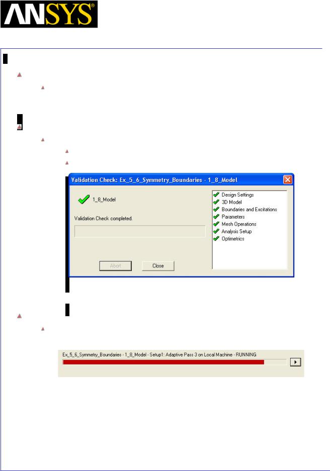
Maxwell v15 |
5.6 |
Example (Magnetostatic) – Symmetry Boundaries
Analysis Setup
There is already Setup1 because it copied from the Full_Model design. Analyze this design by the untouched setting.
Model Validation
To validate the model:
Select the menu item Maxwell 3D > Validation Check
Click the Close button
Note: To view any errors or warning messages, use the Message Manager.
Analyze
To start the solution process:
1. Select the menu item Maxwell 3D > Analyze All
|
|
|
|
|
|
|
|
|
|
|
|
|
|
|
|
|
|
|
|
|
|
|
|
|
|
|
|
|
|
|
|
ANSYS Maxwell 3D Field Simulator v15 User’s Guide |
|
5.6-22 |
|||||
|
|
|
|
|
|
|
|
Maxwell v15 |
5.6 |
Example (Magnetostatic) – Symmetry Boundaries
Solution Data
To view the Solution Data:
Select the menu item Maxwell 3D > Results > Solution Data
In the full model, the number of mesh was 6768, now it becomes 930 meshes in 1/8 models. That means the number of mesh become about 1/7.
|
|
|
|
|
|
|
|
|
|
|
|
ANSYS Maxwell 3D Field Simulator v15 User’s Guide |
|
5.6-23 |
|||
|
|
|
|
|
|
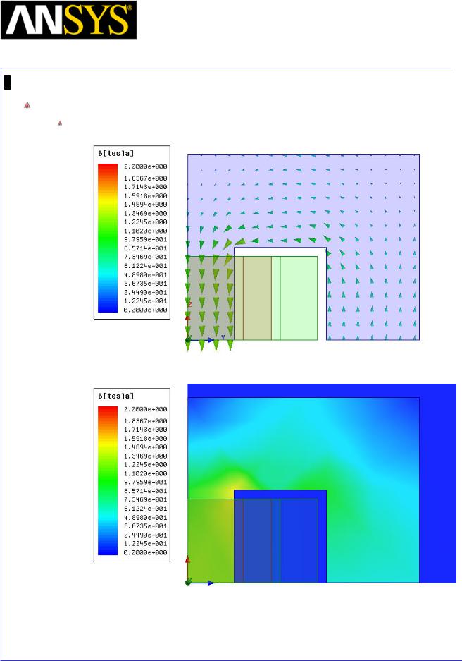
Maxwell v15 |
5.6 |
Example (Magnetostatic) – Symmetry Boundaries
Field Plots
Field plots are already available as design was copied from Full_Model
|
|
|
|
|
|
|
|
|
|
|
|
|
|
|
|
|
|
|
|
|
|
|
|
|
|
|
|
|
|
|
|
ANSYS Maxwell 3D Field Simulator v15 User’s Guide |
|
5.6-24 |
|||||
|
|
|
|
|
|
|
|
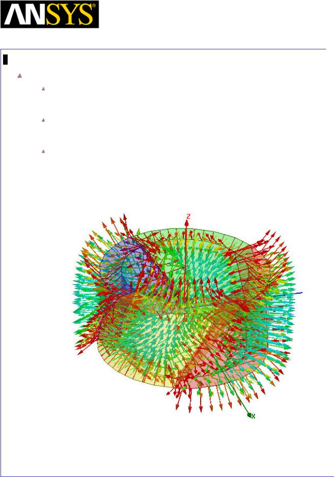
Maxwell v15 |
5.7 |
Example (Magnetostatic) – Permanent Magnet
Magnetization
Permanent Magnet Magnetization
Each object can have the coordinate system that is independent and is arbitrary in Maxwell. The magnetization setting can be done in an arbitrary direction for using this coordinate system.
Moreover, since it is also possible to do the magnetization setting by using the equation and the numeric character data, the user can do a variety of magnetization settings.
This chapter introduces the magnetization setting co-ordinate system, by equations for direction or by character data
|
|
|
|
|
|
|
|
|
|
|
|
|
|
|
|
|
|
|
|
|
|
|
|
|
|
|
|
|
|
|
|
ANSYS Maxwell 3D Field Simulator v15 User’s Guide |
|
5.7-1 |
|||||
|
|
|
|
|
|
|
|

Maxwell v15 |
5.7 |
Example (Magnetostatic) – Permanent Magnet
Magnetization
ANSYS Maxwell Design Environment
The following features of the Ansoft Maxwell Design Environment are used to create the models covered in this topic
3D Solid Modeling
Primitives: Circle, Line
Modeler operations: Sweep
Boolean Operations: Subtract
Analysis
Magnetostatic
Field Overlays:
B Vector Plots
Results
Calculator Expressions Plots
|
|
|
|
|
|
|
|
|
|
|
|
|
|
|
|
|
|
|
|
|
|
|
|
|
|
|
|
|
|
|
|
ANSYS Maxwell 3D Field Simulator v15 User’s Guide |
|
5.7-2 |
|||||
|
|
|
|
|
|
|
|
Maxwell v15 |
5.7 |
Example (Magnetostatic) – Permanent Magnet
Magnetization
Launching Maxwell
To access Maxwell:
1.Click the Microsoft Start button, select Programs, and select Ansoft > Maxwell 15.0 and select Maxwell 15.0
Setting Tool Options
To set the tool options:
Note: In order to follow the steps outlined in this example, verify that the following tool options are set :
1. Select the menu item Tools > Options > Maxwell 3D Options
Maxwell Options Window:
1. Click the General Options tab
Use Wizards for data input when creating new boundaries: Checked
Duplicate boundaries/mesh operations with geometry:
Checked
2.Click the OK button
2.Select the menu item Tools > Options > Modeler Options.
Modeler Options Window:
1. Click the Operation tab
 Automatically cover closed polylines: Checked 2. Click the Display tab
 Default transparency = 0.8 3. Click the Drawing tab
 Edit property of new primitives: Checked 4. Click the OK button
|
|
|
|
|
|
|
|
|
|
|
|
|
|
|
|
|
|
|
|
|
|
|
|
|
|
|
|
|
|
|
|
ANSYS Maxwell 3D Field Simulator v15 User’s Guide |
|
5.7-3 |
|||||
|
|
|
|
|
|
|
|
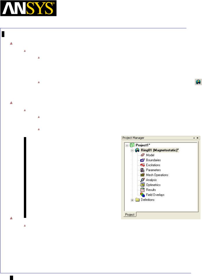
Maxwell v15 |
5.7 |
Example (Magnetostatic) – Permanent Magnet
Magnetization
Opening a New Project
To open a new project:
After launching Maxwell, a project will be automatically created. You can also create a new project using below options.
1.In an Maxwell window, click the On the Standard toolbar, or select the menu item File > New.
Select the menu item Project > Insert Maxwell 3D Design, or click on the icon
Change Design name
To Change Design Name:
Right-click Maxwell3D Design1 at the project manager window and select Rename.
Change the Design Name to Ring01.
Save Project
To save the project:
1.In an Ansoft Maxwell window, select the menu item File > Save As.
2.From the Save As window, type the Filename: Ex_5_7_Permanent_Magnet
3.Click the Save button
|
|
|
|
|
|
|
|
|
|
|
|
|
|
|
|
|
|
|
|
|
|
|
|
|
|
|
ANSYS |
Maxwell 3D Field Simulator v15 User’s Guide |
|
|
5.7-4 |
||||
|
|
|
|
|
|
|
|
|
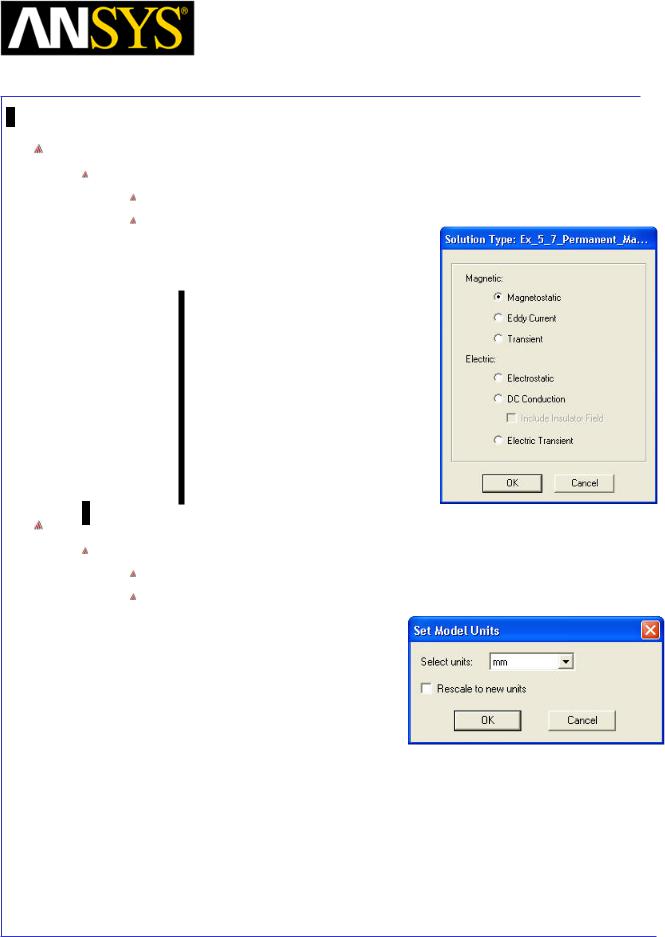
Maxwell v15 |
5.7 |
Example (Magnetostatic) – Permanent Magnet
Magnetization
Set Solution Type
To set the Solution Type:
Select the menu item Maxwell 3D > Solution Type
Solution Type Window:
1.Choose Magnetostatic
2.Click the OK button
Set Model Units
To Set the units:
Select the menu item Modeler > Units
Set Model Units:
1.Select Units: mm
2.Click the OK button
|
|
|
|
|
|
|
|
|
|
|
|
|
|
|
|
|
|
|
|
|
|
|
|
|
|
|
|
|
|
|
|
|
|
|
|
|
|
|
|
|
|
|
|
|
|
|
|
|
|
|
|
|
|
|
|
|
|
|
|
ANSYS Maxwell 3D Field Simulator v15 User’s Guide |
|
5.7-5 |
|||||||
|
|
|
|
|
|
|
|
|
|
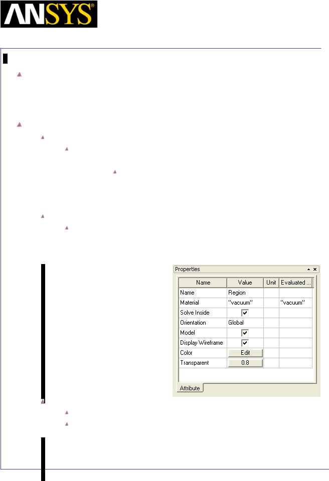
Maxwell v15 |
5.7 |
Example (Magnetostatic) – Permanent Magnet
Magnetization
Example Coordinate system of object and setting for each axis
In this example, it is introduced the magnetization using Coordinate system of object. Material : Mag_North and Mag_South is newly made in this Example.
Create Region
Create a Box region
Select the menu item Draw > Box or click on the icon.
icon.
1. Using the coordinate entry field, enter the box position X: -200, Y: -200, Z: -200 Press the Enter key
2.Using the coordinate entry fields, enter the opposite corner of the box:
 dX: 400, dY: 400, dZ: 400, Press the Enter key Change Attributes
Select the resulting object from the tree and goto Properties window
1.Change the name of the object to Region
2.Display Wireframe: Checked
Hide Region
Select Region from the history tree
Select the menu item View > Visibility > Hide Selection > Active View
|
|
|
|
|
|
|
|
|
|
|
|
|
|
|
|
|
|
|
|
|
ANSYS Maxwell |
3D Field Simulator v15 User’s Guide |
|
5.7-6 |
|||
|
|
|
|
|
|
|
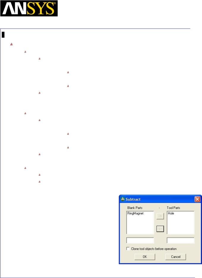
Maxwell v15 |
5.7 |
Example (Magnetostatic) – Permanent Magnet
Magnetization
Create Magnets
Create Circle
Goto menu item Draw > Circle
1. Using the coordinate entry field, enter the center position
X: 0, Y: 0, Z: 0, Press the Enter key
2. Using the coordinate entry field, enter the radius of circle
dX:40 for radius, Press the Enter key
Select the resulting object from the tree and goto Properties window
1.Change the name of the object to RingMagnet
2.Change its color to Blue
Draw another circle
Goto menu item Daw > Circle
1. Using the coordinate entry field, enter the center position
X: 0, Y: 0, Z: 0, Press the Enter key
2. Using the coordinate entry field, enter the radius of circle
dX:30 for radius, Press the Enter key
Select the resulting object from the tree and goto Properties window 1. Change the name of the object to Hole
Subtract Hole from RingMagnet
Select RingMagnet and Hole from the history tree Goto menu item Modeler > Boolean > Subtract
1.Select RingMagnet in Blank Parts
2.Select Hole in Tool Parts
3.Press OK
|
|
|
|
|
|
|
|
|
|
|
|
|
|
|
|
|
|
|
|
|
|
|
|
|
|
|
|
|
|
|
|
ANSYS Maxwell 3D Field Simulator v15 User’s Guide |
|
5.7-7 |
|||||
|
|
|
|
|
|
|
|
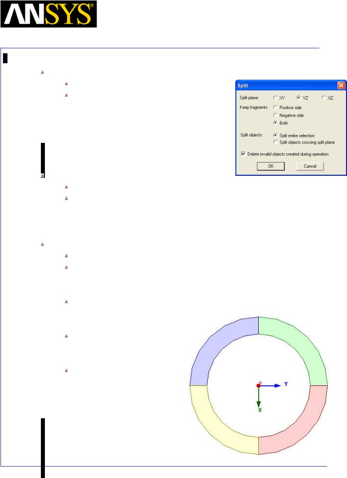
Maxwell v15 |
5.7 |
Example (Magnetostatic) – Permanent Magnet
Magnetization
Split with YZ Plane
Select RingMagnet from the History Tree
Goto menu item Modeler > Boolean > Split
1.Split Plane: Select YZ Plane
2.Keep Fragments: Both
3.Press OK
Split with XZ Plane
Press Ctrl and select RingMagnet and RingMagnet_Split1 from the tree Goto menu item Modeler > Boolean > Split
1.Split Plane: Select XZ Plane
2.Keep Fragments: Both
3.Press OK
Change Attributes
Change the attributes of the four objects resulted from split operation
RingMagnet
1.Name: NorthA
2.Color: Blue
RingMagnet_Split1 |
|
|
|
1. |
Name: SouthA |
|
|
2. |
Color: Yellow |
NorthA |
SouthB |
|
|
||
RingMagnet_Split1_Split1
1.Name: NorthB
2.Color: Red
Ringmagnet_Split2
1.Name: SouthB
2.Color: Green
|
SouthA |
NorthB |
||
|
||||
|
|
|
|
|
|
|
|
|
|
ANSYS Maxwell 3D Field Simulator v15 User’s Guide |
5.7-8 |
||
|
|
|
|
Maxwell v15 |
5.7 |
Example (Magnetostatic) – Permanent Magnet
Magnetization
Create Guide for Sweep
Goto menu item Draw > Line
1. Using the coordinate entry field, enter first vertex positions
X: 0, Y: 0, Z: -20, Press the Enter key
2. Using the coordinate entry field, enter second vertex positions
 X: 0, Y: 0, Z:20, Press the Enter key 3. Press Enter key to Exit
Create Sweep
Select NorthA, NorthB, SouthA, SouthB and Polyline1 from the History Tree
Goto menu item Draw > Sweep > Along Path
1.Set Angle of Twist to 45 degrees
2.Press OK
Note: The 45 degree angle given in sweep command is the Skew Angle of the Magnets. This value will be give through equation in the next exercise of magnetization using equations.
|
|
|
|
|
|
|
|
|
|
|
|
|
|
|
|
|
|
|
|
|
|
|
|
|
|
|
|
|
|
|
|
ANSYS Maxwell 3D Field Simulator v15 User’s Guide |
|
5.7-9 |
|||||
|
|
|
|
|
|
|
|
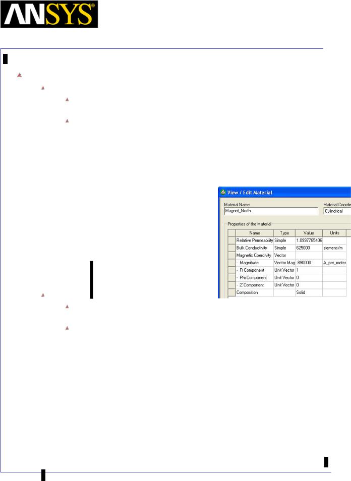
Maxwell v15 |
5.7 |
Example (Magnetostatic) – Permanent Magnet
Magnetization
Create Magnet Materials: Magnet_North, Magnet_South
To Create Material Magnet_North:
Select NorthA and NorthB from the history tree, right click and select Assign Material
In Select Definition window,
1.Type NdFe35 in the Search by Name field
2.Select option Clone Material
3.In View/Edit Material window
1.Material Name Magnet_North
2.Material Coordinate System Cylindrical
3.Magnitude -890000
4.R Component 1
5.Phi Component: 0
6.Z Component 0
7.Press OK
4.select OK to assign the material.
To Create Material Magnet_South:
Select SouthA and SouthB from history tree, right click and select Assign Material
In Select Definition window,
1.Type NdFe35 in the Search by Name field
2.Select option Clone Material
3.In View/Edit Material window
1.Material Name Magnet_South
2.Material Coordinate System Cylindrical
3.Magnitude -890000
4.R Component -1
5.Phi Component: 0
6.Z Component 0
7.Press OK
4.select OK to assign the material.
|
|
|
|
|
ANSYS Maxwell |
3D Field Simulator v15 User’s Guide |
5.7-10 |
||
|
|
|
|
|
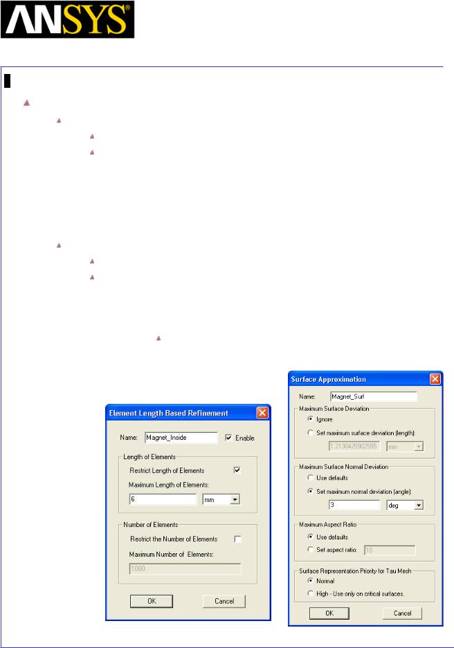
Maxwell v15 |
5.7 |
Example (Magnetostatic) – Permanent Magnet
Magnetization
Apply Mesh Operations
Apply Length Based Mesh Operations
Select NorthA, NorthB, SouthA and SouthB from History Tree
Goto menu item Maxwell 3D > Mesh Operations >Assign > Inside
Selection > Length Based…
1.Name: Magnet_Inside
2.Restrict Length of Elements: Checked
3.Maximum Length of Elements: 6mm
4.Press OK
Apply Surface Approximation
Select NorthA, NorthB, SouthA and SouthB from History Tree
Select menu item Maxwell 3D > Mesh Operations > Assign > Surface
Approximation
1.Name: Magnet_Surf
2.Maximum Surface Normal Deviation
Set maximum normal deviation (angle): 3 deg
3. Press OK
|
|
|
|
|
|
|
|
|
|
|
|
ANSYS Maxwell 3D Field Simulator v15 User’s Guide |
|
5.7-11 |
|||
|
|
|
|
|
|
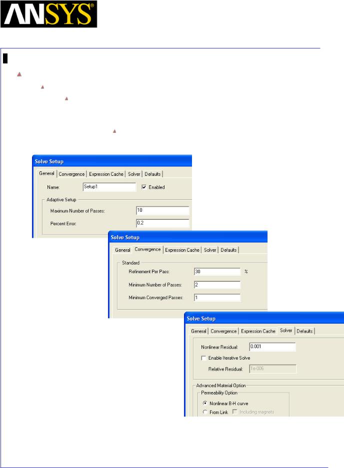
Maxwell v15 |
5.7 |
Example (Magnetostatic) – Permanent Magnet
Magnetization
Analysis Setup
To create an analysis setup:
Select the menu item Maxwell 3D > Analysis Setup > Add Solution Setup In Solve Setup window
1.General tab
Percentage Error: 0.2
2. Press OK
|
|
|
|
|
|
|
|
|
|
|
|
ANSYS Maxwell 3D Field Simulator v15 User’s Guide |
|
5.7-12 |
|||
|
|
|
|
|
|
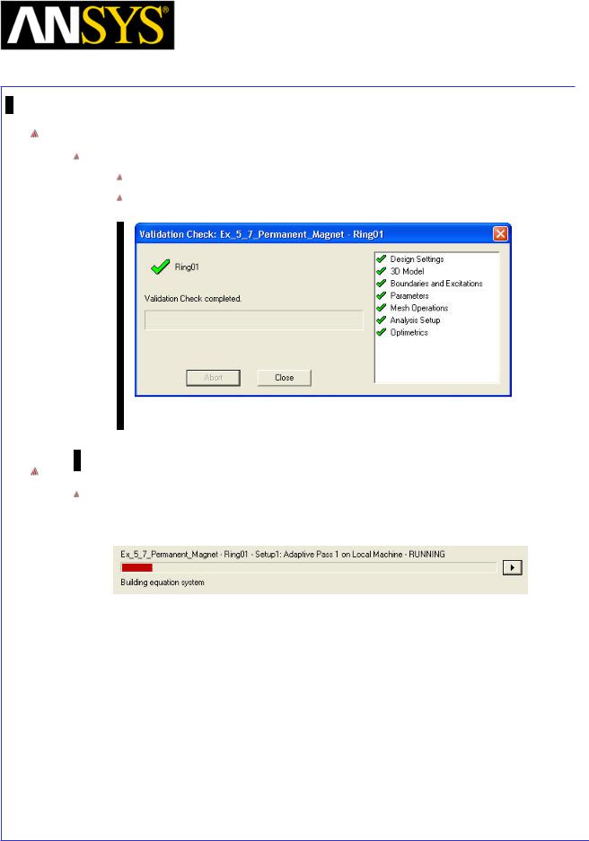
Maxwell v15 |
5.7 |
Example (Magnetostatic) – Permanent Magnet
Magnetization
Model Validation
To validate the model:
Select the menu item Maxwell 3D > Validation Check
Click the Close button
Note: To view any errors or warning messages, use the Message Manager.
Analyze
To start the solution process:
1. Select the menu item Maxwell 3D > Analyze All
|
|
|
|
|
|
|
|
|
|
|
|
|
|
|
|
|
|
|
|
|
|
|
|
|
|
|
|
|
|
|
|
ANSYS Maxwell 3D Field Simulator v15 User’s Guide |
|
5.7-13 |
|||||
|
|
|
|
|
|
|
|
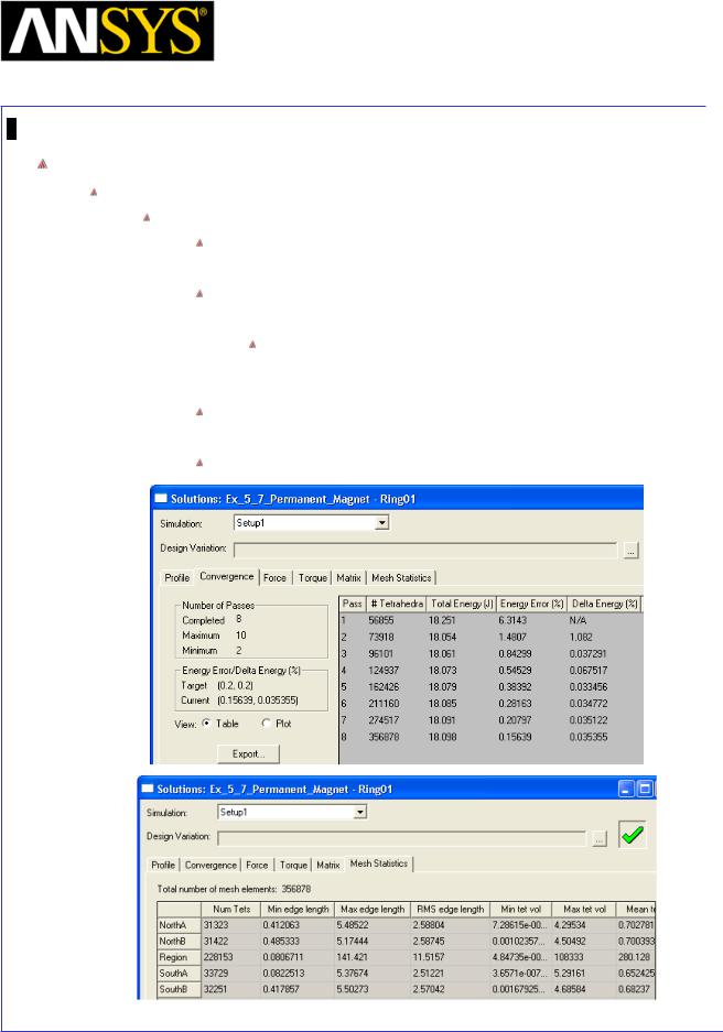
Maxwell v15 |
5.7 |
Example (Magnetostatic) – Permanent Magnet
Magnetization
Solution Data
To view the Solution Data:
Select the menu item Maxwell 3D > Results > Solution Data
To view the Profile:
1. Click the Profile Tab. To view the Convergence:
1. Click the Convergence Tab
Note: The default view is for convergence is Table. Select the Plot radio button to view a graphical representations of the convergence data.
To View Mesh information
1. Click Mesh Statistics Tab Select Close to close the window
|
|
|
|
|
|
|
|
|
|
|
|
|
|
|
|
|
|
|
|
|
|
|
|
|
|
|
|
|
|
|
|
|
|
|
|
|
|
|
|
|
|
|
|
|
|
|
|
|
|
ANSYS Maxwell 3D Field Simulator v15 User’s Guide |
|
5.7-14 |
|||||||
|
|
|
|
|
|
|
|
|
|
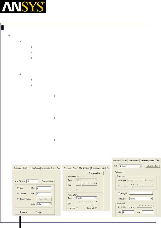
Maxwell v15 |
5.7 |
Example (Magnetostatic) – Permanent Magnet
Magnetization
Vector Plot
Create Vector Plot
Select NorthA, NorthB, SouthA and SouthB from history tree
Select menu item Maxwell 3D > Fields > Fields > B > B_Vector
In Create Field Plot window
1.Plot on surface only : Checked
2.Select Done
Modify Plot Attributes
Double click on the legend to change plot properties
In the window 1. Scale tab
User Limits: Checked
1.Min: 0
2.Max: 1
2.Marker/Arrow tab
Arrow Options
1.Size: Set to appropriate value
2.Map Size: Unchecked
3. Plots tab
Vector Plot
1.Spacing: Set to Maximum
2.Min: 2
3.Max: 4
4.Press Apply and Close
|
|
|
|
|
|
|
|
|
|
|
|
|
|
|
|
|
|
|
|
|
ANSYS Maxwell |
3D Field Simulator v15 User’s Guide |
|
5.7-15 |
|||
|
|
|
|
|
|
|
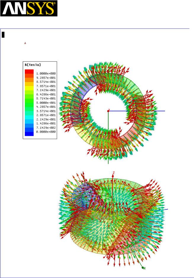
Maxwell v15 |
5.7 |
Example (Magnetostatic) – Permanent Magnet
Magnetization
Each of the magnets is magnetized in radial direction. The direction of magnetization of North magnets is opposite to that of South magnets.
|
|
|
|
|
|
|
|
|
|
|
|
|
|
|
|
|
|
|
|
|
|
|
|
|
|
|
|
|
|
|
|
ANSYS Maxwell 3D Field Simulator v15 User’s Guide |
|
5.7-16 |
|||||
|
|
|
|
|
|
|
|
|
|
|
|
|
Maxwell v15 |
|
5.7 |
||
|
|
|
|
|
Example (Magnetostatic) – Permanent Magnet |
|
|
|
|
|
|
|
|
|
Magnetization |
|
|
|
|
|
|
Create Entities for Rectangular Plot |
|
|
|
||||
|
|
|
|
|
|||||
|
|
|
|
|
|||||
|
|
Turn off automatic covering of polylines |
|
|
|
||||
|
|
|
|
Goto Tools > Options > Modeler Options |
|
|
|
||
1. |
Operation tab |
|
|
|
|||||
|
|
|
|
|
Automatically cover closed polylines: Unchecked |
|
|
|
|
2. |
Press OK |
|
|
|
|||||
|
|
Create Circle |
|
|
|
||||
|
|
|
|
Select menu item Draw > Circle |
|
|
|
||
|
|
|
|
A massage will pop up asking if the entity needs to be created as non |
|||||
|
|
|
|
model object. Select Yes to it. |
|
|
|
||
1. |
Using Co-ordinate entry field Enter the center of the circle |
|
|
|
|||||
|
|
|
|
|
X = 0, Y = 0, Z = -10, Press Enter |
|
|
|
|
2. |
Using Co-ordinate entry field Enter the radius |
|
|
|
|||||
|
|
|
|
|
dX = 40, dY = 0, dZ = 0, Press Enter |
|
|
|
|
|
|
|
|
Select the resulting object from the tree and goto Properties window |
|
|
|
||
1. |
Change the name of the object to CircleA |
|
|
|
|||||
|
|
Create Copies of CircleA along Z axis |
|
|
|
||||
|
|
|
|
Select CircleA from history tree |
|
|
|
||
|
|
|
|
Goto menu item Edit > Duplicate > Along Line |
|
|
|
||
1. |
Using Co-ordinate entry field Enter the first point of duplicate vector |
||||||||
|
|
|
|
|
X = 0, Y = 0, Z = -10, Press Enter |
|
|
|
|
2. |
Using Co-ordinate entry field Enter the second point |
|
|
|
|||||
|
|
|
|
|
dX = 0, dY = 0, dZ = 10, Press Enter |
|
|
|
|
3. |
Set Total Number of Duplicates to 3 |
|
|
|
|||||
|
|
|
|
Select the resulting object from the tree and goto Properties window |
|
|
|
||
1. |
Change the name of the object to CircleB and CircleC |
|
|
|
|||||
|
|
|
|
|
|
|
|
|
|
|
|
|
|
|
|
|
|
|
|
|
|
|
|
|
|
|
|
|
|
|
|
|
|
|
|
|
|
|
|
|
|
|
|
|
|
|
|
|
|
ANSYS Maxwell 3D Field Simulator v15 User’s Guide |
5.7-17 |
||
|
|
|
|

Maxwell v15 |
5.7 |
Example (Magnetostatic) – Permanent Magnet
Magnetization
Create parameter Brad
Create parameter for radial magnetic filed strength
Goto Maxwell 3D > Fileds > Calculator
1.Select Input > Quantity > B
2.Select General > Smooth
3.Select Vector > Scal? > ScalarX
4.Select Input > Function > Scalar > PHI
5.Select Scalar > Trig > Cos
6.Select General > *
7.Select Input > Quantity > B
8.Select General > Smooth
9.Select Vector > Scal? > ScalarY
10.Select Input > Function > Scalar > PHI
11.Select Scalar > Trig > Sin
12.Select General > *
13.Select General > +
14.Select Add and set the name of expression as Brad
15.Press Done
|
|
|
|
|
|
|
|
|
|
|
|
|
|
|
|
|
|
|
|
|
|
|
|
|
|
|
|
|
|
|
|
ANSYS Maxwell 3D Field Simulator v15 User’s Guide |
|
5.7-18 |
|||||
|
|
|
|
|
|
|
|
Maxwell v15 |
5.7 |
Example (Magnetostatic) – Permanent Magnet
Magnetization
Rectangular Plot
To Create Plot:
Select Maxwell 3D > Results > Create Fields Report > Rectangular Plot
In Reports window
1.Geometry: CircleA
2.Trace Tab
1.X axis: Default
2.Y axis
Category: Calculator Expressions
Quantity: Brad
Function: None
3.Select New Report
4.Without closing window, change geometry to CircleB
5.Select Add Trace
6.Change Geomety to CircleC
7.select Add Trace
8.Select Close
|
|
|
|
|
|
|
|
|
|
|
|
|
|
|
|
|
|
|
|
|
|
|
|
|
|
|
|
|
|
|
|
|
|
|
|
|
|
|
|
|
|
|
|
|
|
|
|
|
|
|
|
|
|
|
|
|
|
|
|
|
|
|
|
|
|
|
|
|
|
|
|
|
|
|
|
|
|
|
|
|
|
|
|
|
|
|
|
|
|
|
|
|
|
|
|
ANSYS Maxwell 3D Field Simulator v15 User’s Guide |
|
5.7-19 |
|||||||||
|
|
|
|
|
|
|
|
|
|
|
|
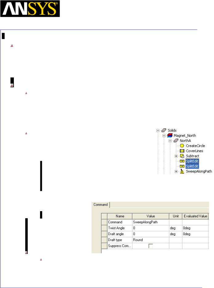
Maxwell v15 |
5.7 |
Example (Magnetostatic) – Permanent Magnet
Magnetization
Example2 Magnetization using the equation
In this example, direction of Magnetization is changed using equation. We will learn to achieve same result as in last exercise without modeling four different poles of Magnet
Prepare Design
Copy Design
1.Select Ring01 design in Project Manager window, right click and select Copy
2.Select project Ex_5_7_Permanent_Magnet in Project Manager window and select Paste
3.Ring2 design is created
Edit Geometry
1.Open the history of NorthA in history tree
2.Select the commands SplitEdit and delete them using Delete key on your keyboard
3.Double click on the command SweepAlongPath from history tree
4.Change Twist Angle from 45 to 0 degress
5.Press OK
Change Attributes
Select the resulting object from the tree and goto Properties window 1. Change the name of the object to RingMagnet
|
|
|
|
|
|
|
|
|
|
|
|
|
|
|
|
|
|
|
|
|
|
|
|
|
|
|
|
|
|
|
|
|
|
|
|
|
|
|
|
ANSYS Maxwell 3D Field Simulator v15 User’s Guide |
|
|
5.7-20 |
||||||
|
|
|
|
|
|
|
|
|
|
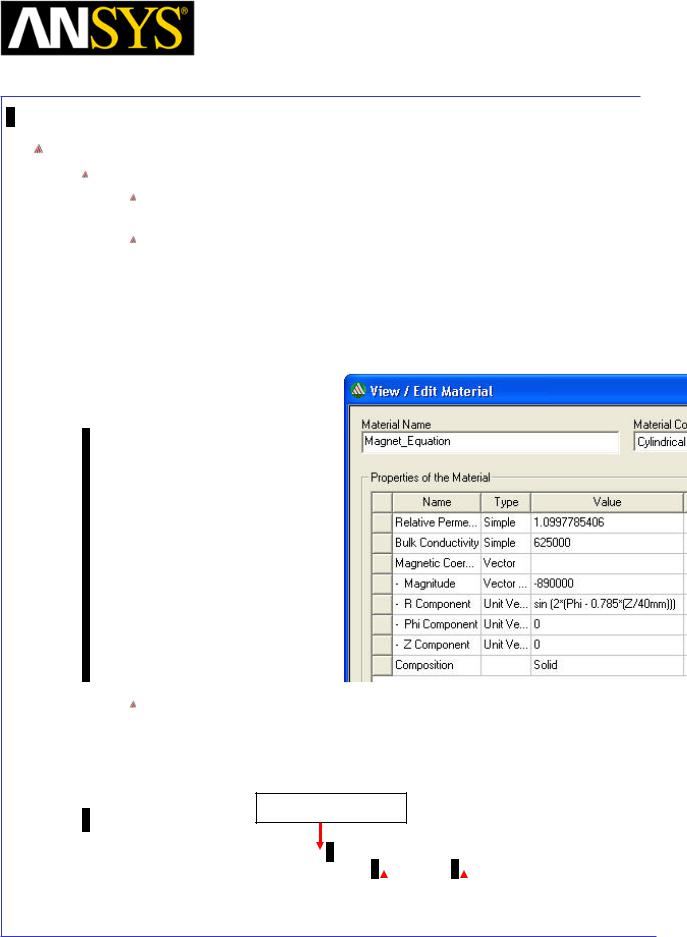
Maxwell v15 |
5.7 |
Example (Magnetostatic) – Permanent Magnet
Magnetization
Create New Material: Magnet_Equation
To Create material Magnet_Equation:
Select RingMagnet from the history tree, right click and select Assign Material
In Select Definition window,
1.Select option Clone Material
2.In View/Edit Material window
1.Material Name Magnet_Equation
2.Magnitude -890000
3.R Component sin (2*(Phi - 0.785*(Z/40mm)))
4.Press OK
3.select OK.
Note About the equation
The equations used in this case is a sine function which switches the value of R from positive to negative with Phi hence altering the direction of magnetization. Rest of the equation gives skew to the direction along Z direction. This gives the field similar to four pole magnet with 45 degree skew modeled in last exercise
Number of Poles / 2
sin (2*(Phi - 0.785*(Z/40mm)))
|
|
|
|
|
|
|
Skew angle in radians[45 deg] |
|
Length of magnet |
|
|
||
|
||||||
|
|
|
|
|
|
|
ANSYS Maxwell 3D Field Simulator v15 User’s Guide |
5.7-21 |
||
|
|
|
|
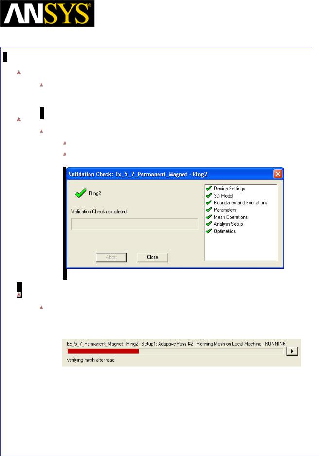
Maxwell v15 |
5.7 |
Example (Magnetostatic) – Permanent Magnet
Magnetization
Analysis Setup
There is already Setup1 because it copied from the Ring01 design. Analyze this design by the untouched setting.
Model Validation
To validate the model:
Select the menu item Maxwell 3D > Validation Check
Click the Close button
Analyze
To start the solution process:
1. Select the menu item Maxwell 3D > Analyze All
|
|
|
|
|
|
|
|
|
|
|
|
|
|
|
|
|
|
|
|
|
|
|
|
|
|
|
|
|
|
|
|
ANSYS Maxwell 3D Field Simulator v15 User’s Guide |
|
5.7-22 |
|||||
|
|
|
|
|
|
|
|
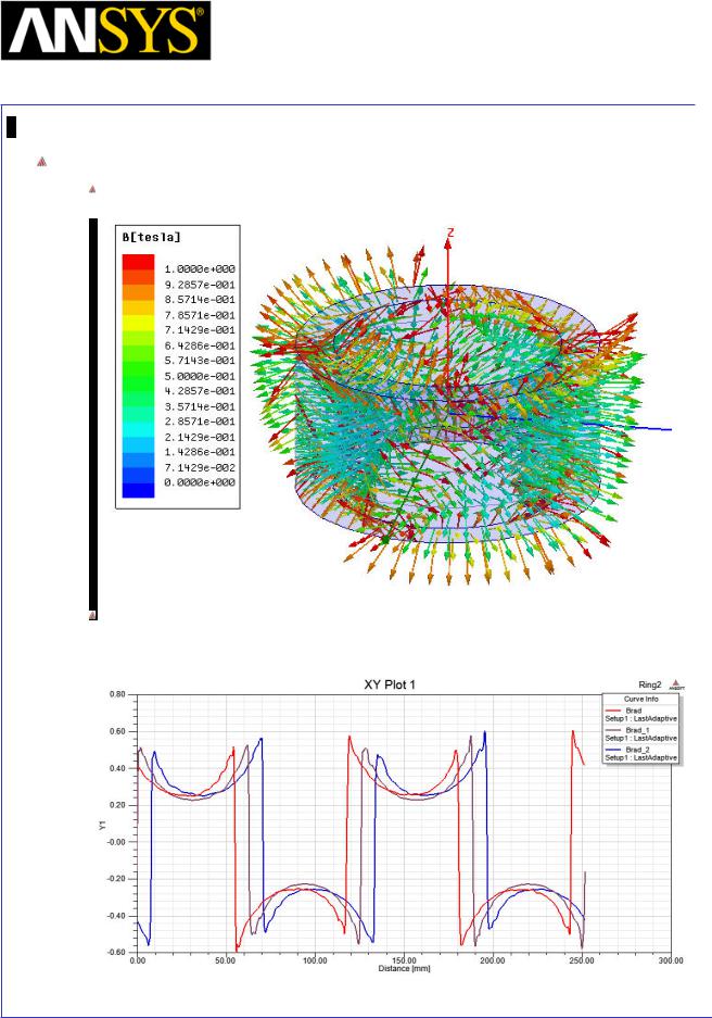
Maxwell v15 |
5.7 |
Example (Magnetostatic) – Permanent Magnet
Magnetization
Results
Double click Field Overlays > B > B_Vector in Project tree to view vector plot
Check the Plots of Brad that we created in last exercise. The results in both cases should be nearly same
|
|
|
|
|
|
|
|
|
|
|
|
|
|
|
|
|
|
|
|
|
|
|
|
|
|
|
|
|
|
|
|
ANSYS Maxwell 3D Field Simulator v15 User’s Guide |
|
5.7-23 |
|||||
|
|
|
|
|
|
|
|
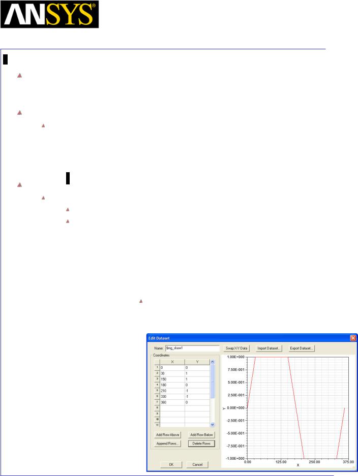
Maxwell v15 |
5.7 |
Example (Magnetostatic) – Permanent Magnet
Magnetization
Example3 Magnetization using Input Curve
In this example, we will learn to vary the magnitude and direction of magnetization by specifying behavior curve to it
Create Design
To copy design
1.Select Ring2 in Project Manager tree, right click and select Copy
2.Select Ex_5_7_Permanent_Magnet in Project Manager window and select Paste
Create New Material : Magnet_Curve
To Create material Magnet_Curve:
Select RingMagnet from tree, right click and select Assign Material In Select Definition window,
1.Select option Clone Material
2.In View/Edit Material window
1.Material Name Magnet_Curve
2.Magnitude -890000 * pwl_periodic( $mg_skew1, 2* (Phi * 180 / PI - 45 *(Z / 40 mm)))
3.Add Dataset window will pop up.
Enter data points as shown in image and Press OK
4.R Component 1
5.Press OK
3.Select OK
|
|
|
|
|
|
|
|
|
|
|
|
ANSYS Maxwell 3D Field Simulator v15 User’s Guide |
|
5.7-24 |
|||
|
|
|
|
|
|
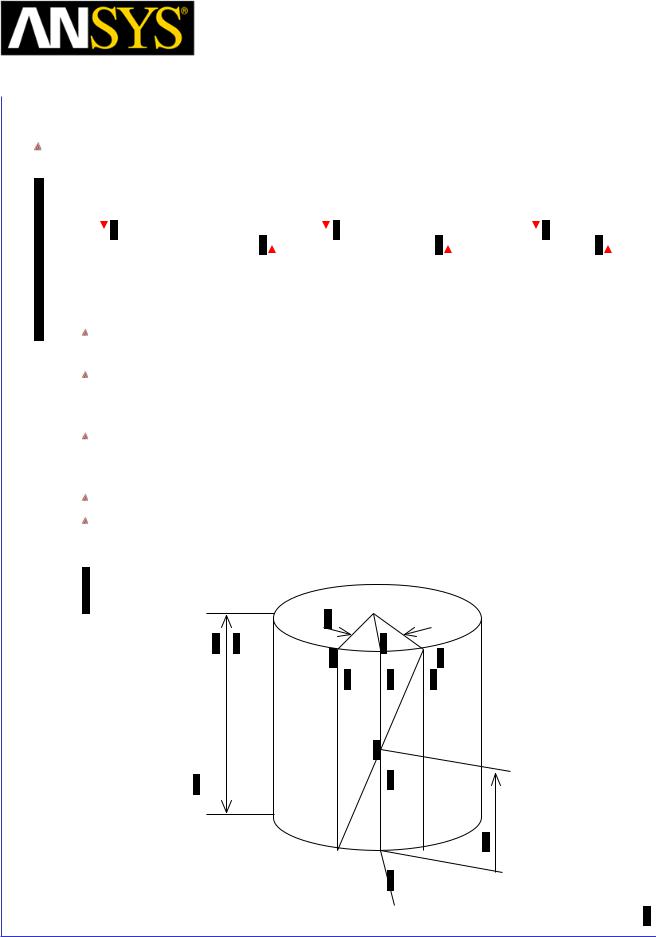
|
|
|
|
|
Maxwell v15 |
|
|
|
|
5.7 |
|||
|
|
|
|
|
Example (Magnetostatic) – Permanent Magnet |
||||||||
|
|
|
|
|
|
|
|
|
Magnetization |
|
|||
|
|
|
Note About the function |
|
|
|
|
|
|
||||
|
|
|
|
|
|
|
|
|
|||||
|
|
|
|
|
|
|
|
|
|||||
|
|
|
|
|
|
|
|
|
|
|
|
||
|
|
|
Magnetization |
|
Number of Poles |
|
0 position |
|
|||||
|
|
|
|
|
|
|
|
|
|
|
|
|
|
|
|
|
|
|
|
|
|
|
|
|
|
|
|
-837999 * pwl_periodic( $mg_skew1, 2* (Phi*180/PI - 45 *((Z- $CoreOrigin / 2 mm)))
|
|
|
|
|
|
|
|
Magnetization wave form |
|
Skew angle[deg] |
|
Length of magnet |
|||
|
|
|
|
|
|
|
|
The function which has been specified in the material definition sets a multiplier $mg_skew1 for the magnitude of magnetic coercivity.
Input curve that we specified varies the multiplier $mg_Skew1 from +1 to -1 with the change in value of Phi. Hence it varies the direction of magnetization of magnets.
Number of poles value will multiply the value of Phi. Hence ensuring value of $mag_skew1 cycles twice in single rotation of Phi. This results two peaks (North Pole) and two valleys (South Pole) giving a four pole magnet.
Moreover, to apply the skew, magnetic data is rotated with Z axis coordinates.
$CoreOrigin defines the Z position where value of $mg_skew becomes zero. In our case this value is 0mm. Hence it is not considered in the function specified.
Skew angle
$Height
CoreOrigin$
 X : Phi = 0
ANSYS Maxwell 3D Field Simulator v15 User’s Guide |
5.7-25 |
||
|
|
|
|
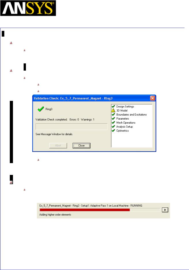
Maxwell v15 |
5.7 |
Example (Magnetostatic) – Permanent Magnet
Magnetization
Analysis Setup
There is already Setup1 because it copied from the Ring2 design. Analyze this design by the untouched setting.
Model Validation
To validate the model:
Select the menu item Maxwell 3D > Validation Check
Click the Close button
Note: A warning will be given by Maxwell informing if coercivity value is set to positive, the direction will be reversed.
Analyze
To start the solution process:
1. Select the menu item Maxwell 3D > Analyze All
|
|
|
|
|
|
|
|
|
|
|
|
ANSYS Maxwell 3D Field Simulator v15 User’s Guide |
|
5.7-26 |
|||
|
|
|
|
|
|
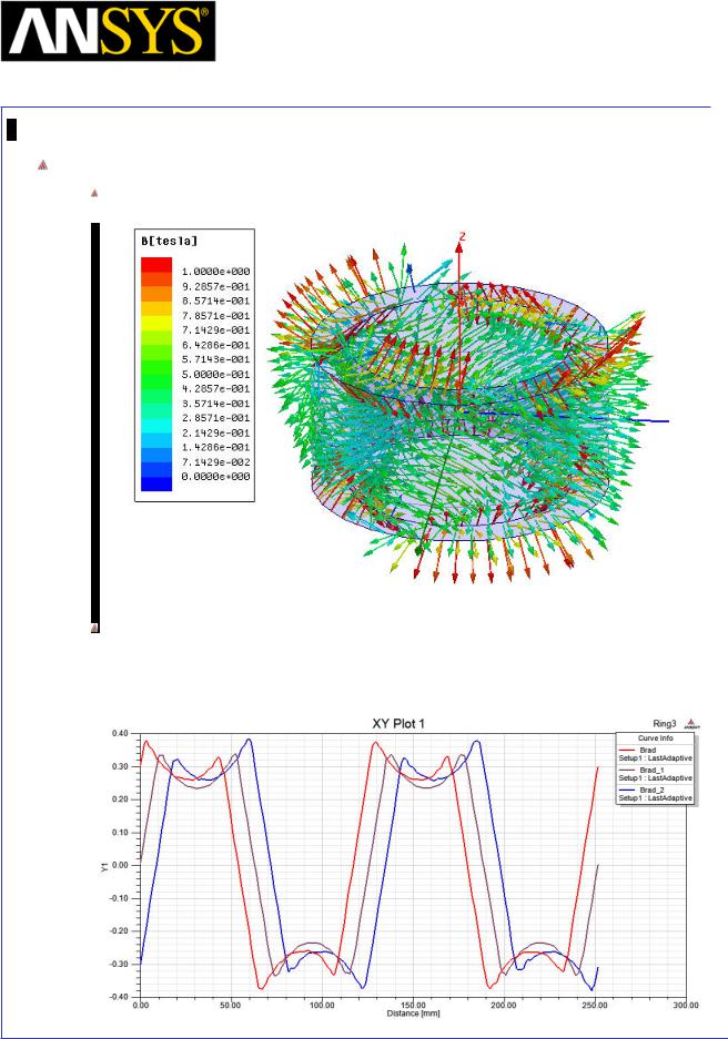
Maxwell v15 |
5.7 |
Example (Magnetostatic) – Permanent Magnet
Magnetization
Results
Double click Field Overlays > B > B_Vector in Project tree to view vector plot
Check the Plots of Brad that we created in last exercise. The difference in the results can be seen. The strength of magnetic filed in radial direction varies with Phi. The function results in for pole magnet as expected.
|
|
|
|
|
|
|
|
|
|
|
|
|
|
|
|
|
|
|
|
|
|
|
|
|
|
|
|
|
|
|
|
ANSYS Maxwell 3D Field Simulator v15 User’s Guide |
|
5.7-27 |
|||||
|
|
|
|
|
|
|
|
Maxwell v15 |
5.8 |
Example (Magnetostatic) – Master/Slave Boundaries
Assigning Master/Slave Boundary Conditions
Boundary Conditions
Boundary conditions enable you to control the characteristics of planes, faces, or interfaces between objects. Boundary conditions are important to understand and are fundamental to solution of Maxwell’s equations.
Master/Slave
Master and slave boundaries enable you to model planes of periodicity where the H-field (E-field for Electrostatic Solver) at every point on the slave boundary surface is forced to match the H-field of every corresponding point on the master boundary surface. The transformation used to map the H-field from the master to the slave is determined by specifying a coordinate system on both the master and slave boundaries.
Considerations
Some considerations for Master/Slave boundaries:
They can only be assigned to planar surfaces.
The geometry of the surface on one boundary must match the geometry on the surface of the other boundary.
Why They are Important
When used properly, Master/Slave boundary conditions can be successfully utilized to reduce the model complexity.
The model complexity usually is directly tied to the solution time and computer resources so it is a competitive advantage to utilize them whenever possible.
|
|
|
|
|
|
|
|
|
|
|
|
|
|
|
|
|
|
|
|
|
|
|
|
|
|
|
|
|
|
|
|
|
|
|
|
|
|
|
|
|
|
|
|
|
|
|
|
|
|
ANSYS Maxwell 3D Field Simulator v15 User’s Guide |
|
5.8-1 |
|||||||
|
|
|
|
|
|
|
|
|
|
Maxwell v15 |
5.8 |
Example (Magnetostatic) – Master/Slave Boundaries
ANSYS Maxwell Design Environment
The following features of the ANSYS Maxwell Design Environment are used to
create the models covered in this topic
3D Solid Modeling
User Defined Primitives (UDP): SRMCore
Surface Operations: Section
Boolean Operations: Separate Bodies
Boundaries/Excitations
Current: Stranded
Boundaries: Master/Slave
Analysis
Magnetostatic
Field Overlays:
H Vector
|
|
|
|
|
|
|
|
|
|
|
|
|
|
|
|
|
|
|
|
|
|
|
|
|
|
|
|
|
|
|
|
ANSYS Maxwell 3D Field Simulator v15 User’s Guide |
|
5.8-2 |
|||||
|
|
|
|
|
|
|
|

Maxwell v15 |
5.8 |
Example (Magnetostatic) – Master/Slave Boundaries
Launching Maxwell
To access Maxwell:
1.Click the Microsoft Start button, select Programs, and select Ansoft > Maxwell 15.0 and select Maxwell 15.0
Setting Tool Options
To set the tool options:
Note: In order to follow the steps outlined in this example, verify that the following tool options are set :
1. Select the menu item Tools > Options > Maxwell 3D Options
Maxwell Options Window:
1. Click the General Options tab
Use Wizards for data input when creating new boundaries: Checked
Duplicate boundaries/mesh operations with geometry:
Checked
2.Click the OK button
2.Select the menu item Tools > Options > Modeler Options.
Modeler Options Window:
1. Click the Operation tab
 Automatically cover closed polylines: Checked 2. Click the Display tab
 Default transparency = 0.8 3. Click the Drawing tab
 Edit property of new primitives: Checked 4. Click the OK button
|
|
|
|
|
|
|
|
|
|
|
|
|
|
|
|
|
|
|
|
|
|
|
|
|
|
|
|
|
|
|
|
ANSYS Maxwell 3D Field Simulator v15 User’s Guide |
|
5.8-3 |
|||||
|
|
|
|
|
|
|
|
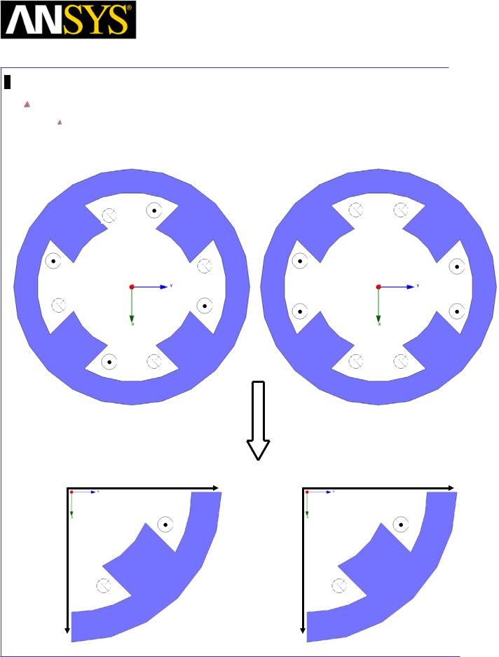
Maxwell v15 |
5.8 |
Example (Magnetostatic) – Master/Slave Boundaries
Designs in the Tutorial
There will be four designs in this example, as shown below. The objective is to demonstrate how to assign Master/Slave boundary conditions and how they can help reduce model complexity and hence solution time.
|
|
|
Design1: Full_Model_1 |
|
|
|
Design2: Full_Model_2 |
|
|
|
|
|
|
||
|
Design3: Quarter_Model_1, Slave=Master |
|
Design4: Quarter_Model_2, Slave=-Master |
||||
|
|
||||||
|
|
|
Slave=Master |
|
|
|
Slave=-Master |
|
|
|
|
|
|
|
|
|
|
|
|
|
|
|
|
Master |
Master |
|
|
|
|
|
|
|
ANSYS Maxwell 3D Field Simulator v15 User’s Guide |
5.8-4 |
||
|
|
|
|
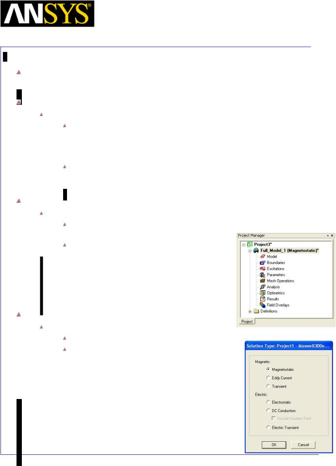
Maxwell v15 |
5.8 |
Example (Magnetostatic) – Master/Slave Boundaries
Problem1: Solve Full_Model_1
Opening a New Project
To open a new project:
After launching Maxwell, a project will be automatically created. You can also create a new project using below options.
1.In an Maxwell window, click the On the Standard toolbar, or select the menu item File > New.
Select the menu item Project > Insert Maxwell 3D Design, or click on the  icon
icon
Change Design name
To Change Design Name:
Right-click Maxwell3D Design1 at the project manager window and select Rename.
Change the Design Name to Full_Model_1
Set Solution Type
To set the Solution Type:
Select the menu item Maxwell 3D > Solution Type
Solution Type Window:
1.Choose Magnetostatic
2.Click the OK button
|
|
|
|
|
|
|
|
|
|
|
|
|
|
|
|
|
|
|
|
|
|
|
|
|
|
|
|
|
|
|
|
|
|
|
|
ANSYS |
Maxwell 3D Field Simulator v15 User’s Guide |
|
5.8-5 |
|||||
|
|
|
|
|
|
|
|
|
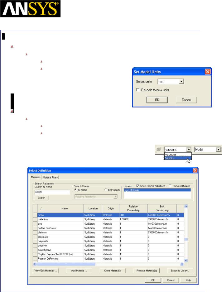
Maxwell v15 |
5.8 |
Example (Magnetostatic) – Master/Slave Boundaries
Set Model Units
To Set the units:
Select the menu item Modeler > Units
Set Model Units:
1.Select Units: mm
2.Click the OK button
Set Default Material
To set the default material:
Using the 3D Modeler Materials toolbar, choose Select
In Select Definition window,
1.Type nickel in the Search by Name field
2.Click the OK button
|
|
|
|
|
|
|
|
|
|
|
|
|
|
|
|
|
|
|
|
|
|
|
|
|
|
|
|
|
|
|
|
ANSYS Maxwell 3D Field Simulator v15 User’s Guide |
|
5.8-6 |
|||||
|
|
|
|
|
|
|
|
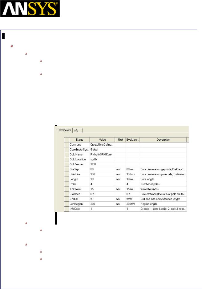
Maxwell v15 |
5.8 |
Example (Magnetostatic) – Master/Slave Boundaries
Create Stator and Coils
To create Stator and Coils
Select the menu item Draw > User Defined Primitives > SysLib > RMxprt > SRMCore
In User Defined Primitive Operation window
1.For the value of DiaGap, type: 80, Click the Tab key to accept
2.For the value of DiaYoke, type: 150, Click the Tab key to accept
3.For the value of Length, type: 10, Click the Tab key to accept
4.For the value of Poles, type: 4, Click the Tab key to accept
5.For the value of InfoCore, type: 1, Click the Tab key to accept
6.Click the OK button
Change Attributes
Select the resulting object from the tree and goto Properties window 1. Change the name of the object to Stator
Separate Objects
Select the object Stator from the history tree
Select the menu item Modeler > Boolean > Separate Bodies
|
|
|
|
|
|
|
|
|
|
|
|
|
|
|
|
|
|
|
|
|
|
|
|
|
|
|
|
|
|
|
|
ANSYS Maxwell 3D Field Simulator v15 User’s Guide |
|
5.8-7 |
|||||
|
|
|
|
|
|
|
|
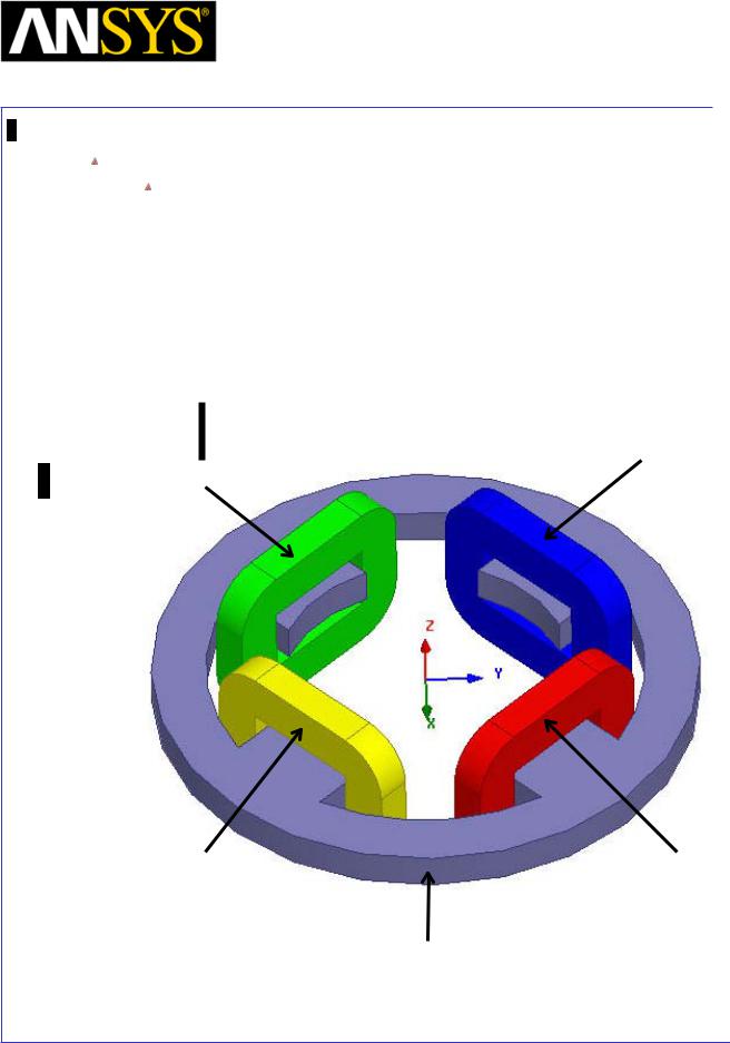
Maxwell v15 |
5.8 |
Example (Magnetostatic) – Master/Slave Boundaries
Change Attributes
Select the objects from the tree and goto Properties window
1.Change the name of the object Stator_Separate1 to Coil1 and Color to Red
2.Change the name of the object Stator_Separate2 to Coil3 and Color to Green
3.Change the name of the object Stator_Separate3 to Coil2 and Color to Blue
4.Change the name of the object Stator_Separate4 to Coil4 and Color to Yellow
Coil2
Coil3
Coil4 |
Coil1 |
|
Stator
|
|
|
|
|
|
|
|
|
|
|
|
ANSYS Maxwell 3D Field Simulator v15 User’s Guide |
|
5.8-8 |
|||
|
|
|
|
|
|
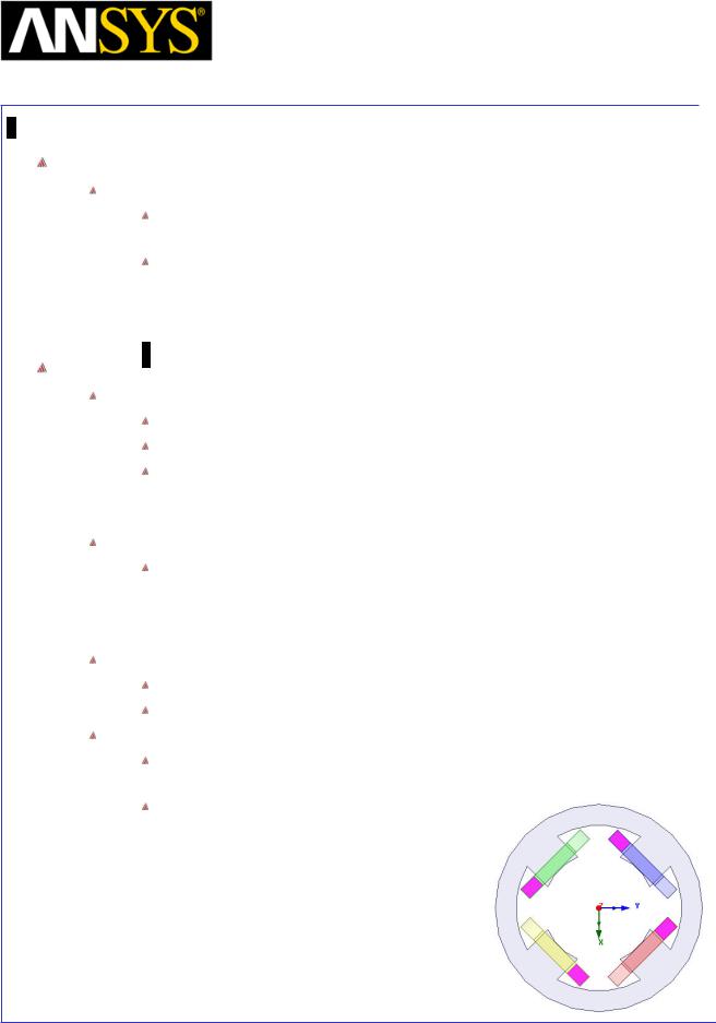
Maxwell v15 |
5.8 |
Example (Magnetostatic) – Master/Slave Boundaries
Assign Material for Coils
To Assign Material
Press Ctrl and select the objects Coil1, Coil2, Coil3 and Coil4, right click and select Assign Material
In Select Definition window,
1.Type copper in the Search by Name field
2.Click the OK button
Create Coil Terminals
Create Section
Press Ctrl and select the objects Coil1, Coil2, Coil3 and Coil4 from the tree
Select the menu item Modeler > Surface >Section
In Section window,
1.Section Plane: XY
2.Click the OK button
Change Attributes
Select the sheets from the tree and goto Properties window
1.Change the name of the sheets Coil1_Section1, Coil2_Section1, Coil3_Section1 and Coil4_Section1 to Term1, Term2, Term3 and Term4 respectively
Separate Sections
Press Ctrl and select sheets Term1, Term2, Term3 and Term4 from tree
Select the menu item Modeler > Boolean > Separate Bodies
Delete Extra Sheets
Press Ctrl and select the sheets Term1_Separate1, Term2_Separate1, Term3_Separate1 and Term4_Separate1 from the tree
Select the menu item Edit > Delete
|
|
|
|
|
|
|
|
|
|
|
|
|
|
|
|
|
|
|
|
|
|
|
|
|
|
|
|
|
|
|
|
ANSYS Maxwell 3D Field Simulator v15 User’s Guide |
|
5.8-9 |
|||||
|
|
|
|
|
|
|
|
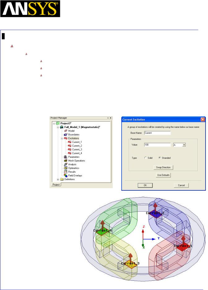
Maxwell v15 |
5.8 |
Example (Magnetostatic) – Master/Slave Boundaries
Create Excitations
To Assign Excitations
Press Ctrl and select the sheets Term1, Term2, Term3 and Term4
Select the menu item Maxwell 3D > Excitations > Assign > Current
In Current Excitation window,
1.Name: Current
2.Value: 100 A
3.Type: Stranded
4.Direction: Positive Z(Use Swap Direction if needed)
5.Press OK
|
|
|
|
|
|
|
|
|
|
|
|
ANSYS Maxwell 3D Field Simulator v15 User’s Guide |
|
5.8-10 |
|||
|
|
|
|
|
|
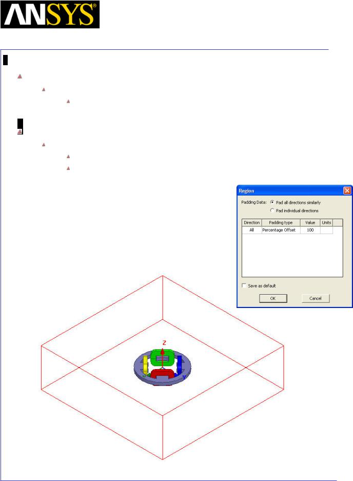
Maxwell v15 |
5.8 |
Example (Magnetostatic) – Master/Slave Boundaries
Set Default Material
To Set Default Material
Using the 3D Modeler Materials toolbar, choose Vacuum
Define Region
Create Simulation Region
Select the menu item Draw > Region
In Region window,
1.Pad all directions similarly: Checked
2.Padding Type: Percentage Offset
3.Value: 100
4.Press OK
|
|
|
|
|
|
|
|
|
|
|
|
|
|
|
|
|
|
|
|
|
|
|
|
|
|
|
|
|
|
|
|
ANSYS Maxwell 3D Field Simulator v15 User’s Guide |
|
5.8-11 |
|||||
|
|
|
|
|
|
|
|
Maxwell v15 |
5.8 |
Example (Magnetostatic) – Master/Slave Boundaries
Analysis Setup
To create an analysis setup:
Select the menu item Maxwell 3D > Analysis Setup > Add Solution Setup
Solution Setup Window:
1. Click the OK button to accept all default settings.
Save Project
To save the project:
1.In an Ansoft Maxwell window, select the menu item File > Save As.
2.From the Save As window, type the Filename: Ex_5_8_Master_Slave
3.Click the Save button
Model Validation
To validate the model:
Select the menu item Maxwell 3D > Validation Check
Click the Close button
Note: To view any errors or warning messages, use the Message Manager.
Analyze
To start the solution process:
1. Select the menu item Maxwell 3D > Analyze All
|
|
|
|
|
|
|
|
|
|
|
|
ANSYS Maxwell 3D Field Simulator v15 User’s Guide |
|
5.8-12 |
|||
|
|
|
|
|
|
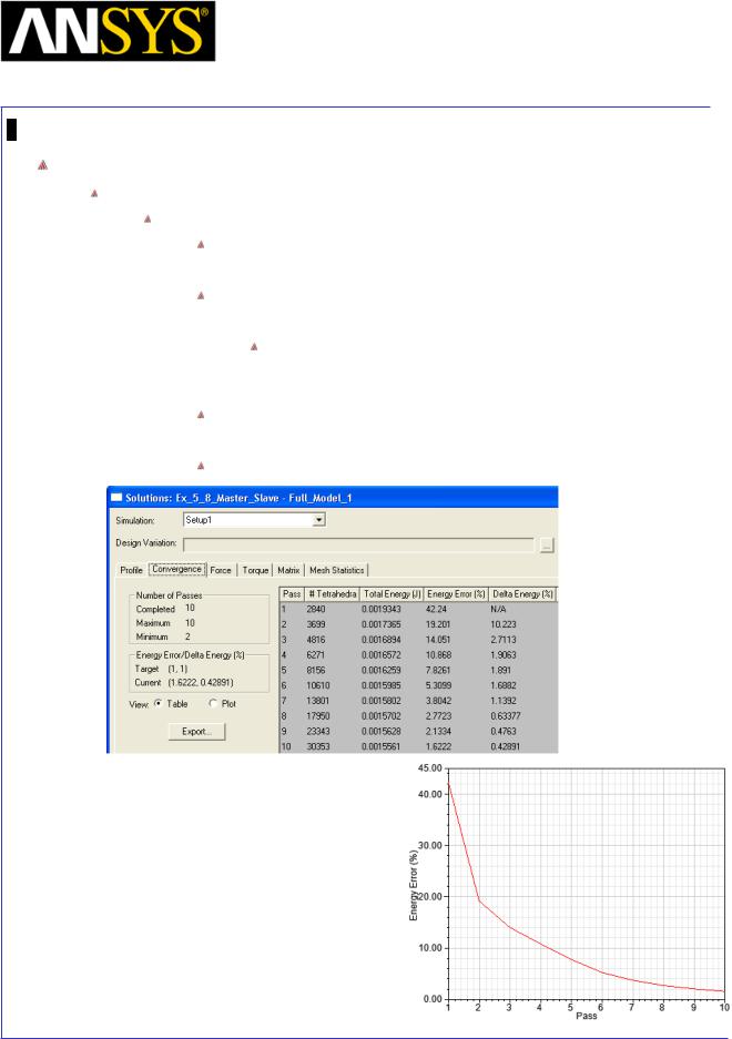
Maxwell v15 |
5.8 |
Example (Magnetostatic) – Master/Slave Boundaries
Solution Data
To view the Solution Data:
Select the menu item Maxwell 3D > Results > Solution Data
To view the Profile:
1. Click the Profile Tab. To view the Convergence:
1. Click the Convergence Tab
Note: The default view is for convergence is Table. Select the Plot radio button to view a graphical representations of the convergence data.
To View Mesh information
1. Click Mesh Statistics Tab Select Close to close the window
|
|
|
|
|
|
|
|
|
|
|
|
|
|
|
|
|
|
|
|
|
|
|
|
|
|
|
|
|
|
|
|
ANSYS Maxwell 3D Field Simulator v15 User’s Guide |
|
5.8-13 |
|||||
|
|
|
|
|
|
|
|
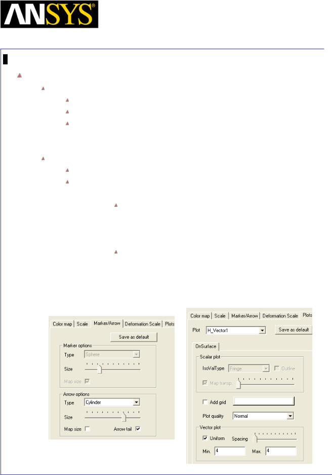
Maxwell v15 |
5.8 |
Example (Magnetostatic) – Master/Slave Boundaries
Vector Plot
Create Vector Plot
Select Global:XY plane from history tree
Select menu item Maxwell 3D > Fields > Fields > H > H_Vector
In Create Field Plot window
1.In Volume: AllObjects
2.Select Done
Modify Plot Attributes
Double click on the legend to change plot properties
In the window
1. Marker/Arrow tab Arrow Options
1.Size: Set to appropriate value
2.Map Size: Unchecked
2. Plots tab
Vector Plot
1.Spacing: Set to Minimum
2.Min: 4
3.Max: 4
3.Press Apply and Close
|
|
|
|
|
|
|
|
|
|
|
|
ANSYS Maxwell 3D Field Simulator v15 User’s Guide |
|
5.8-14 |
|||
|
|
|
|
|
|
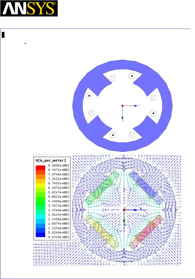
Maxwell v15 |
5.8 |
Example (Magnetostatic) – Master/Slave Boundaries
H-field vector plot will appear, which is the result of the current excitation shown below
|
|
|
|
|
|
|
|
|
|
|
|
|
|
|
|
|
|
|
|
|
|
|
|
|
|
|
|
|
|
|
|
ANSYS Maxwell 3D Field Simulator v15 User’s Guide |
|
5.8-15 |
|||||
|
|
|
|
|
|
|
|
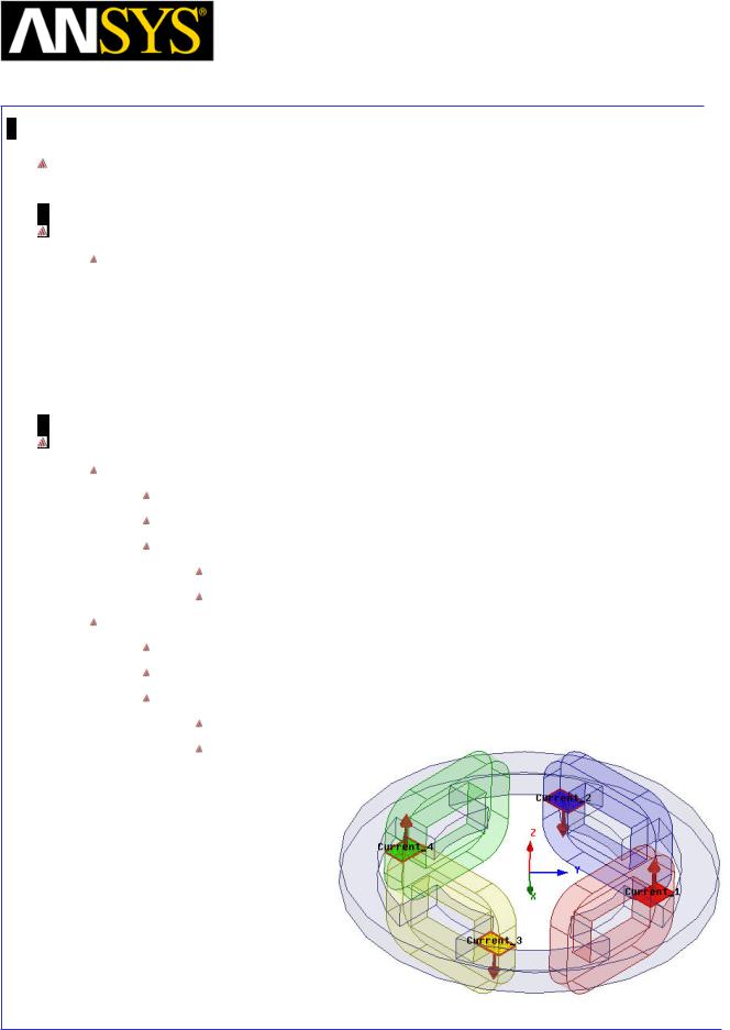
Maxwell v15 |
5.8 |
Example (Magnetostatic) – Master/Slave Boundaries
Problem 2: Solve Full_Model_2
Create Symmetry Design
Copy Design
1.Select the design Full_Model_1 in Project Manager window, right click and select Copy
2.Select project Ex_5_8_Master_Slave in Project Manager window and select Paste
3.Change the name of the design to Full_Model_2
Modify Excitations
Modify Direction of Current in Coil2
Expand the tree Excitations in Project Manager window
Double click on excitation corresponding to Coil2 (in this case Current2)
In Current Excitation window,
Use Swap Direction (Set direction to Negative Z)
Press Ok
Modify Direction of Current in Coil4
Expand the tree Excitations in Project Manager window
Double click on excitation corresponding to Coil4 (in this case Current3)
In Current Excitation window,
Use Swap Direction (Set direction to Negative Z) Press Ok
|
|
|
|
|
|
|
|
|
|
|
|
|
|
|
|
|
|
|
|
|
|
|
|
|
|
|
|
|
|
|
|
ANSYS Maxwell 3D Field Simulator v15 User’s Guide |
|
5.8-16 |
|||||
|
|
|
|
|
|
|
|

Maxwell v15 |
5.8 |
Example (Magnetostatic) – Master/Slave Boundaries
Analysis Setup
There is already Setup1 because it copied from the Full_Model_2 design. Analyze this design by the untouched setting.
Model Validation
To validate the model:
Select the menu item Maxwell 3D > Validation Check
Click the Close button
Note: To view any errors or warning messages, use the Message Manager.
Analyze
To start the solution process:
1. Select the menu item Maxwell 3D > Analyze All
|
|
|
|
|
|
|
|
|
|
|
|
ANSYS Maxwell 3D Field Simulator v15 User’s Guide |
|
5.8-17 |
|||
|
|
|
|
|
|
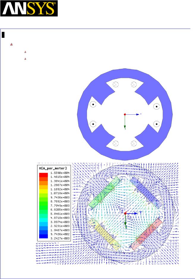
Maxwell v15 |
5.8 |
Example (Magnetostatic) – Master/Slave Boundaries
Field Plots
Field plots are already available as design was copied from Full_Model_1 Double click Field Overlays > Field > H > H_Vector_1 from Project Manager tree
|
|
|
|
|
|
|
|
|
|
|
|
|
|
|
|
|
|
|
|
|
|
|
|
|
|
|
|
|
|
|
|
ANSYS Maxwell 3D Field Simulator v15 User’s Guide |
|
5.8-18 |
|||||
|
|
|
|
|
|
|
|
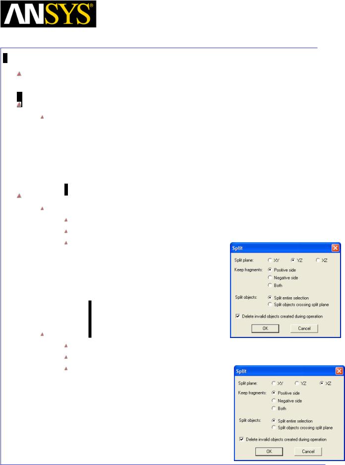
Maxwell v15 |
5.8 |
Example (Magnetostatic) – Master/Slave Boundaries
Problem 3: Solve Quarter Geometry with Master = Slave
Create Symmetry Design
Copy Design
1.Select the design Full_Model_1 in Project Manager window, right click and select Copy
2.Select project Ex_5_8_Master_Slave in Project Manager window and select Paste
3.Change the name of the design to Quarter_Model_1
Split Model for 1/4th Section
Divide by YZ Plane
Select the menu item Edit > Select All
Select the menu item Modeler > Boolean >Split
In Split window
1.Split plane: YZ
2.Keep fragments: Positive side
3.Split objects: Split entire selection
4.Press OK
Divide by XZ Plane
Select the menu item Edit > Select All
Select the menu item Modeler > Boolean >Split
In Split window
1.Split plane: XZ
2.Keep fragments: Positive side
3.Split objects: Split entire selection
4.Press OK
|
|
|
|
|
|
|
|
|
|
|
|
|
|
|
|
|
|
|
|
|
|
|
|
|
|
|
|
|
|
|
|
ANSYS Maxwell 3D Field Simulator v15 User’s Guide |
|
5.8-19 |
|||||
|
|
|
|
|
|
|
|
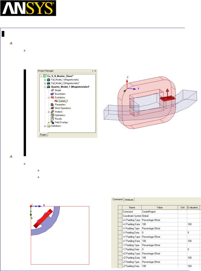
Maxwell v15 |
5.8 |
Example (Magnetostatic) – Master/Slave Boundaries
Excitations
As we are considering 1/4th section of geometry, apart from Coil1, all other coils have been removed. Excitation assigned to Coil1 is available from the first simulation.
Modify Region
To Modify Region
Select the menu item Draw > Region
In Properties window of Region
1.Change -X Padding Data to 0
2.Change -Y Padding Data to 0
3.Press OK
|
|
|
|
|
|
|
|
|
|
|
|
ANSYS Maxwell 3D Field Simulator v15 User’s Guide |
|
5.8-20 |
|||
|
|
|
|
|
|
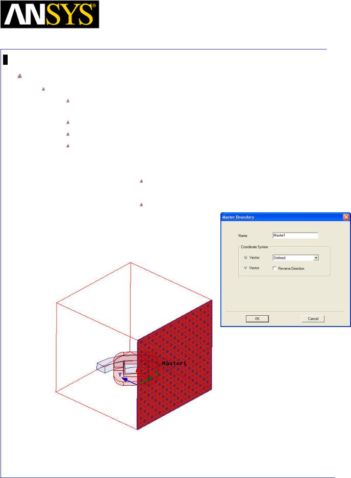
Maxwell v15 |
5.8 |
Example (Magnetostatic) – Master/Slave Boundaries
Assign Boundaries
Assign Master Boundary
Select the menu item Edit > Select > Faces or press F from the keyboard to change selection to faces
Select the face of the Region which touch with XZ Plane
Select the menu item Maxwell 3D > Boundaries > Assign > Master
In Master Boundary window
1.U Vector: Set the option to New Vector
1.Using the coordinate entry fields, enter the first vertex
X: 0, Y: 0, Z: 0, Press the Enter key
2. Using the coordinate entry fields, enter the second vertex
dX: 0, dY: 0, dZ: 1, Press the Enter key
2. Press OK
|
|
|
|
|
|
|
|
|
|
|
|
|
|
|
|
|
|
|
|
|
|
|
|
|
|
|
|
|
|
|
|
ANSYS Maxwell 3D Field Simulator v15 User’s Guide |
|
5.8-21 |
|||||
|
|
|
|
|
|
|
|
Maxwell v15 |
5.8 |
Example (Magnetostatic) – Master/Slave Boundaries
Assign Slave Boundary
Select the face of the Region with which touch with YZ Plane
Select the menu item Maxwell 3D > Boundaries > Assign > Slave
In Slave Boundary window
1.Master boundary: Select Master1
2.U Vector: Set the option to New Vector
1.Using the coordinate entry fields, enter the first vertex
X: 0, Y: 0, Z: 0, Press the Enter key
2. Using the coordinate entry fields, enter the second vertex dX: 0, dY: 0, dZ: 1, Press the Enter key
3.Relation: Select Hs=Hm
4.Press OK
|
|
|
|
|
|
|
|
|
|
|
|
|
|
|
|
|
|
|
|
|
|
|
|
|
|
|
|
|
|
|
|
ANSYS Maxwell 3D Field Simulator v15 User’s Guide |
|
5.8-22 |
|||||
|
|
|
|
|
|
|
|
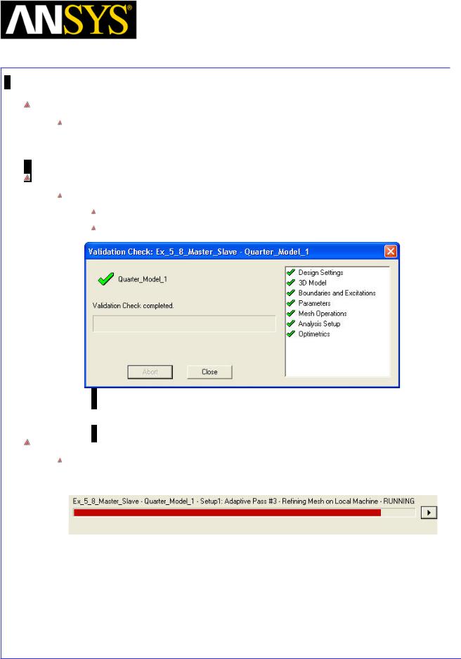
Maxwell v15 |
5.8 |
Example (Magnetostatic) – Master/Slave Boundaries
Analysis Setup
There is already Setup1 because it copied from the Full_Model_1 design. Analyze this design by the untouched setting.
Model Validation
To validate the model:
Select the menu item Maxwell 3D > Validation Check
Click the Close button
Note: To view any errors or warning messages, use the Message Manager.
Analyze
To start the solution process:
1. Select the menu item Maxwell 3D > Analyze All
|
|
|
|
|
|
|
|
|
|
|
|
ANSYS Maxwell 3D Field Simulator v15 User’s Guide |
|
5.8-23 |
|||
|
|
|
|
|
|
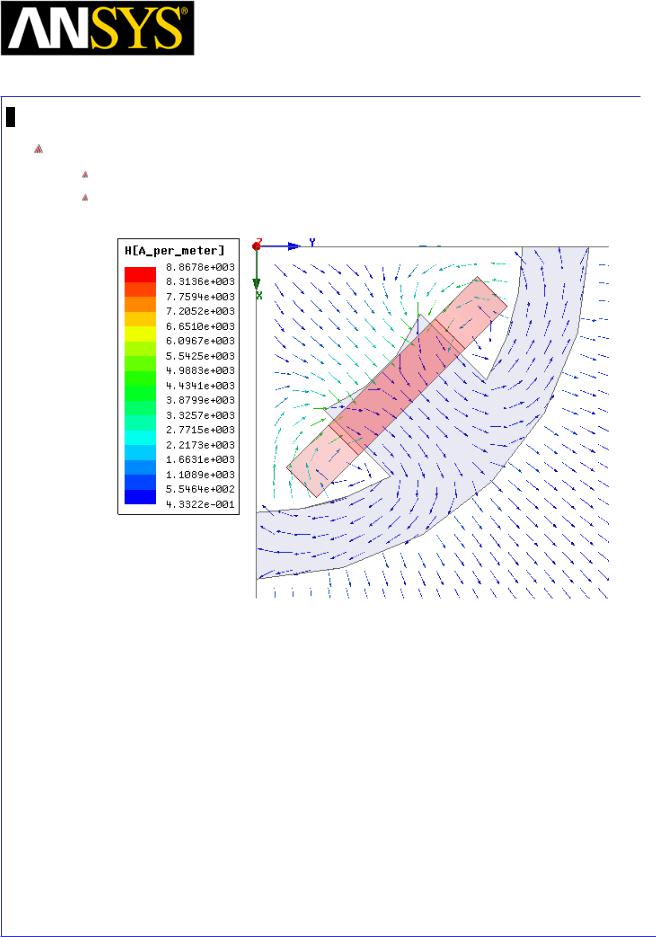
Maxwell v15 |
5.8 |
Example (Magnetostatic) – Master/Slave Boundaries
Field Plots
Field plots are already available as design was copied from Full_Model_1 Double click Field Overlays > Field > H > H_Vector_1 from Project Manager tree
|
|
|
|
|
|
|
|
|
|
|
|
ANSYS Maxwell 3D Field Simulator v15 User’s Guide |
|
5.8-24 |
|||
|
|
|
|
|
|
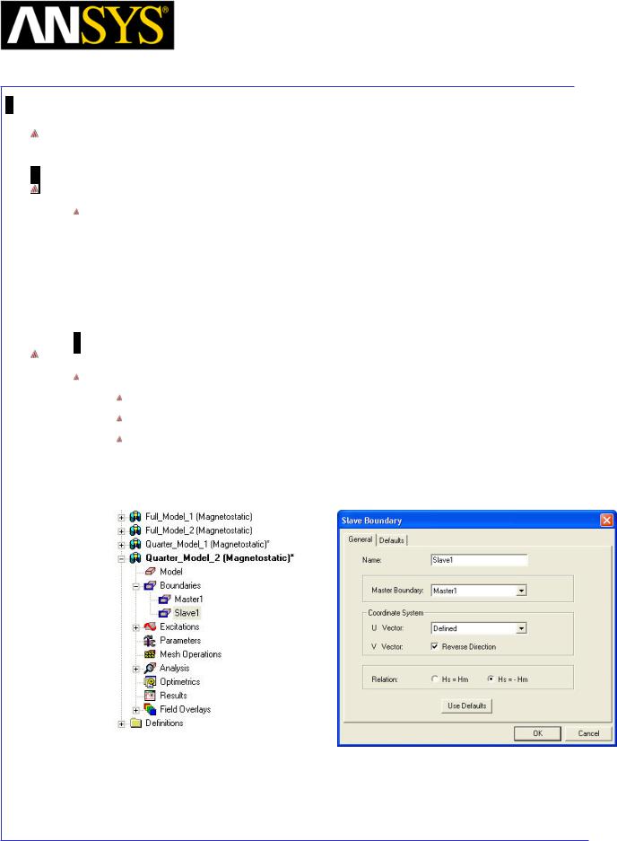
Maxwell v15 |
5.8 |
Example (Magnetostatic) – Master/Slave Boundaries
Problem 3: Solve Quarter Geometry with Salve= -Master
Create Design
Copy Design
1.Select the design Quarter_Model_1 in Project Manager window, right click and select Copy
2.Select project Ex_5_8_Master_Slave in Project Manager window and select Paste
3.Change the name of the design to Quarter_Model_2
Modify Boundary
Modify Slave Boundary to achieve Slave = -Master
Expand the tree Boundaries in Project Manager window
Double click on Slave1 from the tree
In Slave Boundary window
1.Relation: Change to Hs=-Hm
2.Press OK
|
|
|
|
|
|
|
|
|
|
|
|
|
|
|
|
|
|
|
|
|
|
|
|
|
|
|
|
|
|
|
|
|
|
|
|
|
|
|
|
|
|
|
|
|
|
|
|
|
|
ANSYS Maxwell 3D Field Simulator v15 User’s Guide |
|
5.8-25 |
|||||||
|
|
|
|
|
|
|
|
|
|
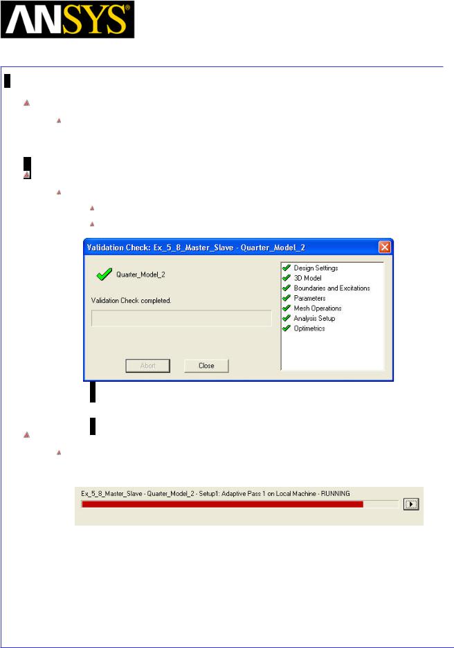
Maxwell v15 |
5.8 |
Example (Magnetostatic) – Master/Slave Boundaries
Analysis Setup
There is already Setup1 because it copied from the Quarter_Model_1 design. Analyze this design by the untouched setting.
Model Validation
To validate the model:
Select the menu item Maxwell 3D > Validation Check
Click the Close button
Note: To view any errors or warning messages, use the Message Manager.
Analyze
To start the solution process:
1. Select the menu item Maxwell 3D > Analyze All
|
|
|
|
|
|
|
|
|
|
|
|
ANSYS Maxwell 3D Field Simulator v15 User’s Guide |
|
5.8-26 |
|||
|
|
|
|
|
|
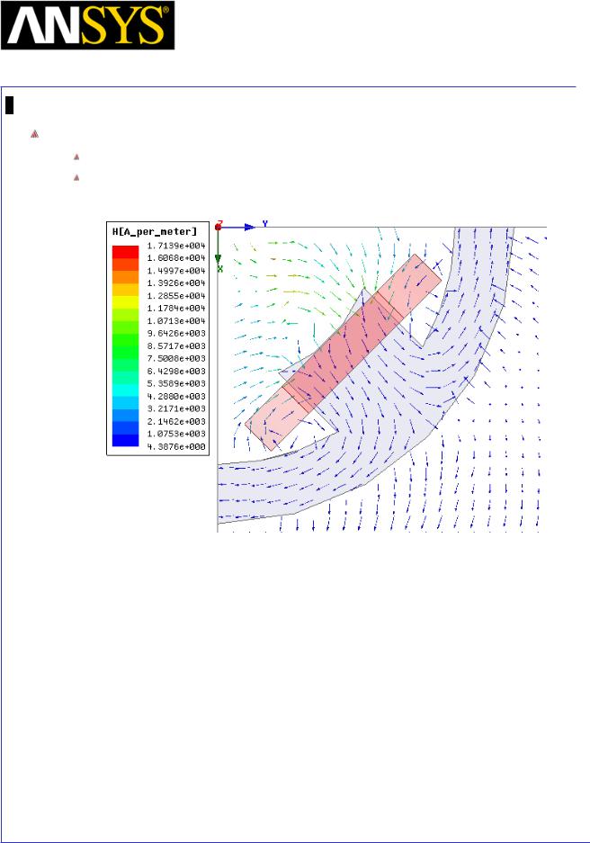
Maxwell v15 |
5.8 |
Example (Magnetostatic) – Master/Slave Boundaries
Field Plots
Field plots are already available as design was copied from Quarter_Model_1 Double click Field Overlays > Field > H > H_Vector_1 from Project Manager tree
|
|
|
|
|
|
|
|
|
|
|
|
ANSYS Maxwell 3D Field Simulator v15 User’s Guide |
|
5.8-27 |
|||
|
|
|
|
|
|
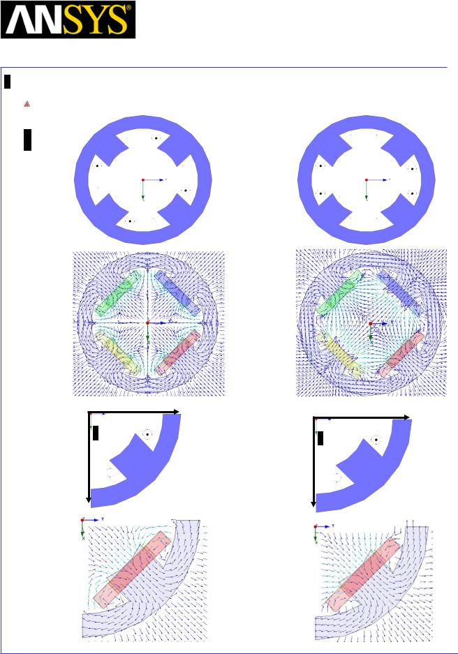
Maxwell v15 |
5.8 |
Example (Magnetostatic) – Master/Slave Boundaries
Topic Summary
Slave=Master |
Slave=-Master |
|
Master |
Master |
|
|
|
|
|
|
|
|
|
|
|
|
|
ANSYS Maxwell 3D Field Simulator v15 User’s Guide |
|
5.8-28 |
|||
|
|
|
|
|
|

|
Maxwell v15 |
|
6.0 |
|
Chapter 6.0 – Eddy Current |
|
|
|
|
|
|
|
|
|
|
Chapter 6.0 – Eddy Current Examples
6.1 – Asymmetrical Conductor with a Hole
6.2 – Radiation Boundary
6.3 - Instantaneous Forces on Busbars
|
|
|
|
|
|
|
|
|
|
|
|
|
|
|
|
|
|
|
|
|
|
|
|
|
|
|
|
|
|
|
|
ANSYS Maxwell 3D Field Simulator v15 User’s Guide |
|
6.0 |
|
||||
|
|
|
|
|
|
|
|
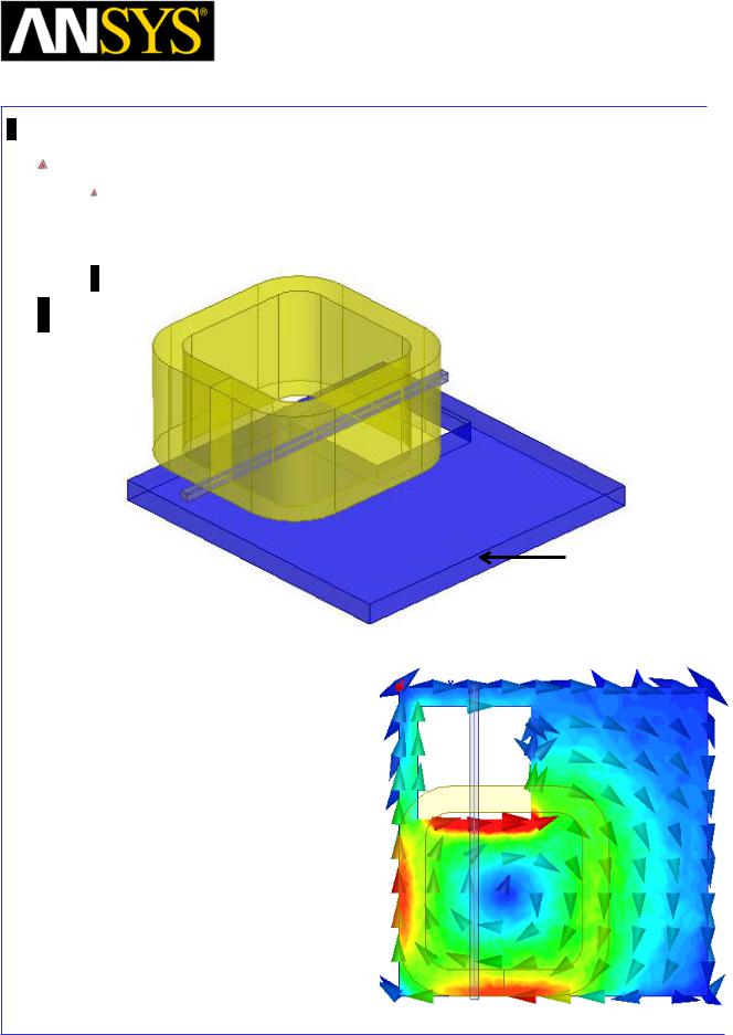
Maxwell v15 |
6.1 |
Example (Eddy Current) – Asymmetric Conductor
The Asymmetrical Conductor with a Hole
This example is intended to show you how to create and analyze an Asymmetrical Conductor with a Hole using the Eddy Current solver in the Ansoft Maxwell 3D Design Environment.
 Coil (Copper)
Stock (Aluminum)
|
|
|
|
|
|
|
|
|
|
|
|
ANSYS Maxwell 3D Field Simulator v15 User’s Guide |
|
6.1-1 |
|||
|
|
|
|
|
|

Maxwell v15 |
6.1 |
Example (Eddy Current) – Asymmetric Conductor
ANSYS Maxwell Design Environment
The following features of the ANSYS Maxwell Design Environment are used to
create the models covered in this topic
3D Solid Modeling
Primitives: Box
Surface Operations: Section
Boolean Operations: Subtract, Separate Bodies
Boundaries/Excitations
Current: Stranded
Analysis
Eddy Current
Results
Calculator Expressions
Plots
Field Overlays:
Mag_J
|
|
|
|
|
|
|
|
|
|
|
|
|
|
|
|
|
|
|
|
|
|
|
|
|
|
|
|
|
|
|
|
ANSYS Maxwell 3D Field Simulator v15 User’s Guide |
|
6.1-2 |
|||||
|
|
|
|
|
|
|
|
Maxwell v15 |
6.1 |
Example (Eddy Current) – Asymmetric Conductor
Launching Maxwell
To access Maxwell:
1.Click the Microsoft Start button, select Programs, and select Ansoft > Maxwell 15.0 and select Maxwell 15.0
Setting Tool Options
To set the tool options:
Note: In order to follow the steps outlined in this example, verify that the following tool options are set :
1. Select the menu item Tools > Options > Maxwell 3D Options
Maxwell Options Window:
1. Click the General Options tab
Use Wizards for data input when creating new boundaries: Checked
Duplicate boundaries/mesh operations with geometry:
Checked
2.Click the OK button
2.Select the menu item Tools > Options > Modeler Options.
Modeler Options Window:
1. Click the Operation tab
 Automatically cover closed polylines: Checked 2. Click the Display tab
 Default transparency = 0.8 3. Click the Drawing tab
 Edit property of new primitives: Checked 4. Click the OK button
|
|
|
|
|
|
|
|
|
|
|
|
|
|
|
|
|
|
|
|
|
|
|
|
|
|
|
|
|
|
|
|
ANSYS Maxwell 3D Field Simulator v15 User’s Guide |
|
6.1-3 |
|||||
|
|
|
|
|
|
|
|

Maxwell v15 |
6.1 |
Example (Eddy Current) – Asymmetric Conductor
Opening a New Project
To open a new project:
After launching Maxwell, a project will be automatically created. You can also create a new project using below options.
1.In an Maxwell window, click the On the Standard toolbar, or select the menu item File > New.
Select the menu item Project > Insert Maxwell 3D Design, or click on the icon
Set Solution Type
To set the Solution Type:
Select the menu item Maxwell 3D > Solution Type
Solution Type Window:
1.Choose Eddy Current
2.Click the OK button
|
|
|
|
|
|
|
|
|
|
|
|
|
|
|
|
|
|
|
|
|
|
|
|
|
|
|
|
|
|
|
|
|
|
|
|
|
|
|
|
|
|
|
|
|
|
|
|
|
|
|
|
|
|
|
|
|
|
|
|
ANSYS Maxwell 3D Field Simulator v15 User’s Guide |
|
6.1-4 |
|||||||
|
|
|
|
|
|
|
|
|
|
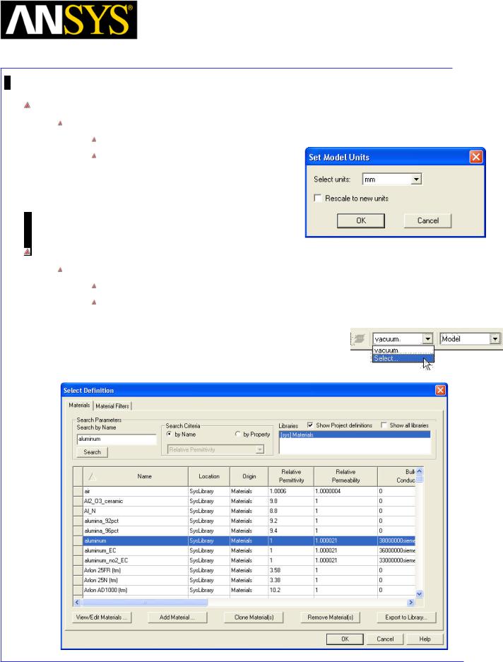
Maxwell v15 |
6.1 |
Example (Eddy Current) – Asymmetric Conductor
Set Model Units
To Set the units:
Select the menu item Modeler > Units
Set Model Units:
1.Select Units: mm
2.Click the OK button
Set Default Material
To set the default material:
Using the 3D Modeler Materials toolbar, choose Select
In Select Definition window,
1.Type aluminum in the Search by Name field
2.Click the OK button
|
|
|
|
|
|
|
|
|
|
|
|
|
|
|
|
|
|
|
|
|
|
|
|
|
|
|
|
|
|
|
|
ANSYS Maxwell 3D Field Simulator v15 User’s Guide |
|
6.1-5 |
|||||
|
|
|
|
|
|
|
|
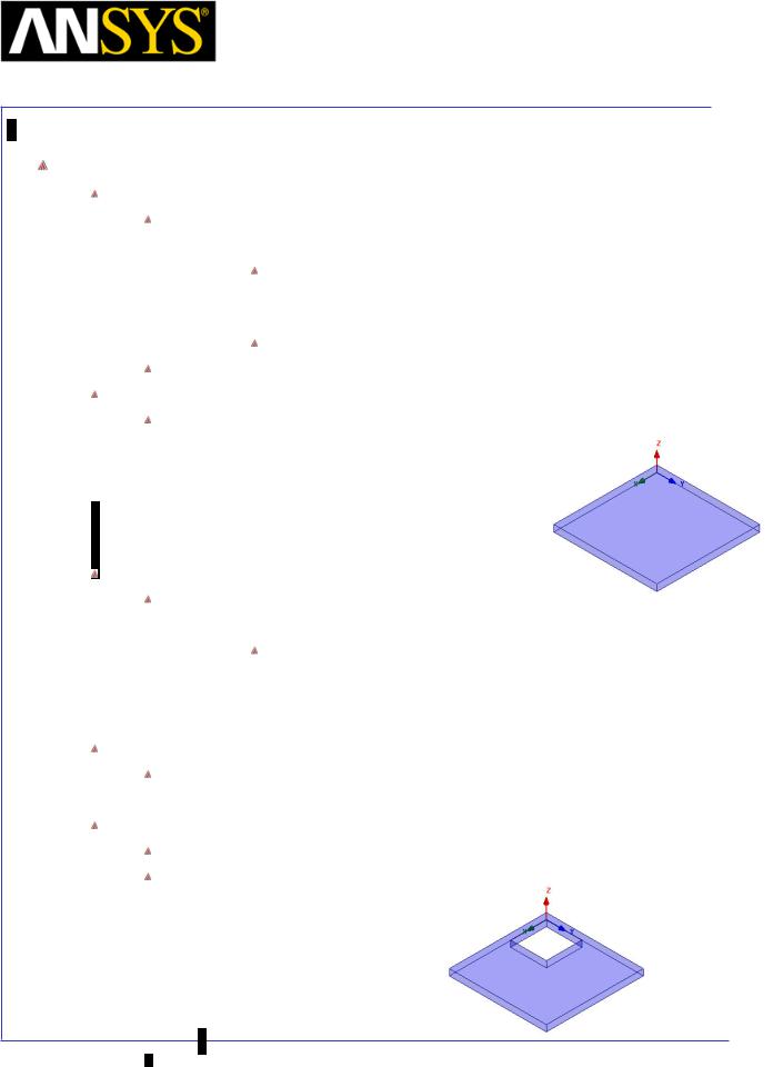
Maxwell v15 |
6.1 |
Example (Eddy Current) – Asymmetric Conductor
Create Stock
Create Box
Select the menu item Draw > Box
1. Using the coordinate entry fields, enter the box position X: 0, Y: 0, Z: 0, Press the Enter key
2.Using the coordinate entry fields, enter the opposite corner of the box:
dX: 294, dY: 294, dZ: 19, Press the Enter key
Select the menu item View > Visibility > Fit All > Active View.
Change Attributes
Select the resulting object from the tree and goto Properties window
1.Change the name of the object to Stock
2.Change its color to Blue
Create Hole
Select the menu item Draw > Box
1. Using the coordinate entry fields, enter the box position X: 18, Y: 18, Z: 0, Press the Enter key
2.Using the coordinate entry fields, enter the opposite corner of the box:
 dX: 108, dY: 108, dZ: 19, Press the Enter key Change Attributes
Select the resulting object from the tree and goto Properties window 1. Change the name of the object to Hole
Subtract Objects
Select the menu item Edit > Select All
Select the menu item, Modeler > Boolean > Subtract
1.Blank Parts: Stock
2.Tool Parts: Hole
3.Click the OK button
|
|
|
|
|
|
|
|
|
|
|
|
|
|
|
|
|
|
|
|
|
|
|
|
ANSYS Maxwell 3D Field Simulator v15 User’s Guide |
|
|
6.1-6 |
||||
|
|
|
|
|
|
|
|
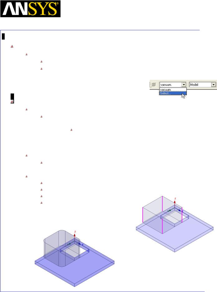
Maxwell v15 |
6.1 |
Example (Eddy Current) – Asymmetric Conductor
Set Default Material
To set the default material:
Using the 3D Modeler Materials toolbar, choose Select
In Select Definition window,
1.Type Copper in the Search by Name field
2.Click the OK button
Create Coil
Create Coil_Hole
Select the menu item Draw > Box
1. Using the coordinate entry fields, enter the box position X: 119, Y: 25, Z: 49, Press the Enter key
2.Using the coordinate entry fields, enter the opposite corner of the box:
 dX: 150, dY: 150, dZ: 100, Press the Enter key Change Attributes
Select the object from the tree and goto Properties window 1. Change the name of the object to Coil_Hole
Create Fillets
Select the menu item Edit > Select > Edges or press “E” from keyboard
Press Ctrl and select the edges as shown in image
Select the menu item Modeler > Fillet In Fillet Properties Window,
1.Fillet Radius: 25mm
2.Setback Distance: 0mm
3.Click the OK button
|
|
|
|
|
|
|
|
|
|
|
|
|
|
|
|
|
|
|
|
|
|
|
|
|
|
|
|
|
|
|
|
|
|
|
|
|
|
|
|
|
|
|
|
|
|
|
|
|
|
|
|
|
|
|
|
|
|
|
|
|
|
|
|
|
|
|
|
|
|
|
|
|
|
|
|
|
|
|
|
|
|
|
|
ANSYS Maxwell 3D Field Simulator v15 User’s Guide |
|
6.1-7 |
|||||||||
|
|
|
|
|
|
|
|
|
|
|
|
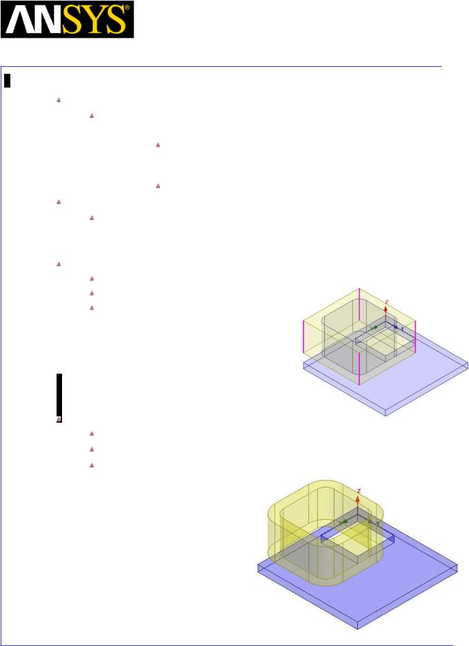
Maxwell v15 |
6.1 |
Example (Eddy Current) – Asymmetric Conductor
Create Coil
Select the menu item Draw > Box
1. Using the coordinate entry fields, enter the box position X: 94, Y: 0, Z: 49, Press the Enter key
2.Using the coordinate entry fields, enter the opposite corner of the box:
dX: 200, dY: 200, dZ: 100, Press the Enter key
Change Attributes
Select the object from the tree and goto Properties window
1.Change the name of the object to Coil
2.Change its color to Yellow
Create Fillets
Press Ctrl and select the edges as shown in image
Select the menu item Modeler > Fillet
In Fillet Properties Window,
1.Fillet Radius: 50mm
2.Setback Distance: 0mm
3.Click the OK button
Subtract Objects
Select the menu item Edit > Select > Objects or press “O” from keyboard
Pres Ctrl and select the objects Coil and Coil_Hole from history tree Select the menu item, Modeler > Boolean > Subtract
1.Blank Parts: Coil
2.Tool Parts: Coil_Hole
3.Click the OK button
|
|
|
|
|
|
|
|
|
|
|
|
|
|
|
|
|
|
|
|
|
|
|
|
|
|
|
|
|
|
|
|
ANSYS Maxwell 3D Field Simulator v15 User’s Guide |
|
6.1-8 |
|||||
|
|
|
|
|
|
|
|
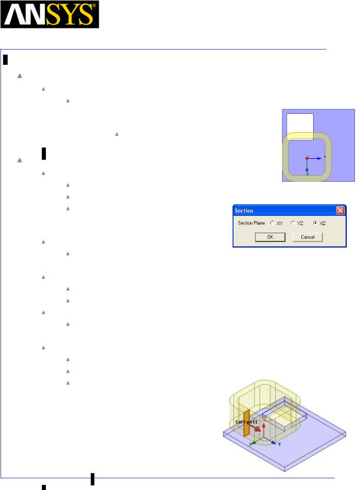
Maxwell v15 |
6.1 |
Example (Eddy Current) – Asymmetric Conductor
Create Offset Coordinate System
To Create Offset Coordinate System
Select the menu item Modeler > Coordinate System > Create > Relative CS > Offset
1. Using the coordinate entry fields, enter the origin X: 200, Y: 100, Z: 0, Press the Enter key
Create Excitations
Create Section of coil for assigning Current
Select the object Coil from the history tree
Select the menu item Modeler > Surface > Section
In Section window,
1.Section Plane: XZ
2.Click the OK button
Change Attributes
Select the object Coil_Section1 from the tree and goto Properties window 1. Change the name of the object to Coil_Terminal
Separate Sheets
Select the sheet Coil_Terminal
Select the menu item Modeler > Boolean > Separate Bodies
Delete Extra Sheets
Select the sheet Coil_Terminal_Seperate1 from the tree
 Select the menu item Edit >Delete Assign Excitations
Select the sheet Coil_Terminal from the history tree
Select the menu item Maxwell 3D > Excitations > Assign > Current
In Current Excitation window,
1.Name: Current1
2.Value: 2742
3.Phase: 0
4.Type: Stranded
5.Current Direction: positive Y (Use Swap Direction if needed)
6.Press OK
|
|
|
|
|
|
|
|
|
|
|
|
|
|
ANSYS Maxwell |
3D Field Simulator v15 User’s Guide |
|
|
6.1-9 |
||
|
|
|
|
|
|
|
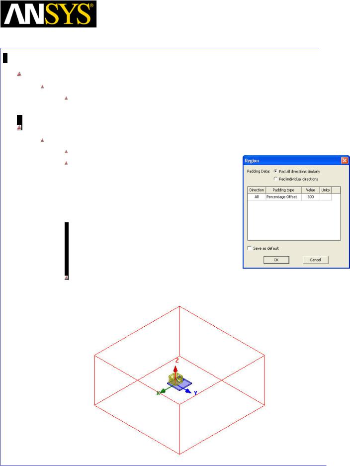
Maxwell v15 |
6.1 |
Example (Eddy Current) – Asymmetric Conductor
Set Default Material
To Set Default Material
Using the 3D Modeler Materials toolbar, choose Vacuum
Define Region
Create Simulation Region
Select the menu item Draw > Region
In Region window,
1.Pad all directions similarly: Checked
2.Padding Type: Percentage Offset
3.Value: 300
4.Press OK
Note: For all Maxwell 3D projects a solution space must be defined. Unless a partial model (like a motor wedge) is used, a region is usually created as described above.
|
|
|
|
|
|
|
|
|
|
|
|
|
|
|
|
|
|
|
|
|
|
|
|
|
|
|
|
|
|
|
|
ANSYS Maxwell 3D Field Simulator v15 User’s Guide |
|
6.1-10 |
|||||
|
|
|
|
|
|
|
|
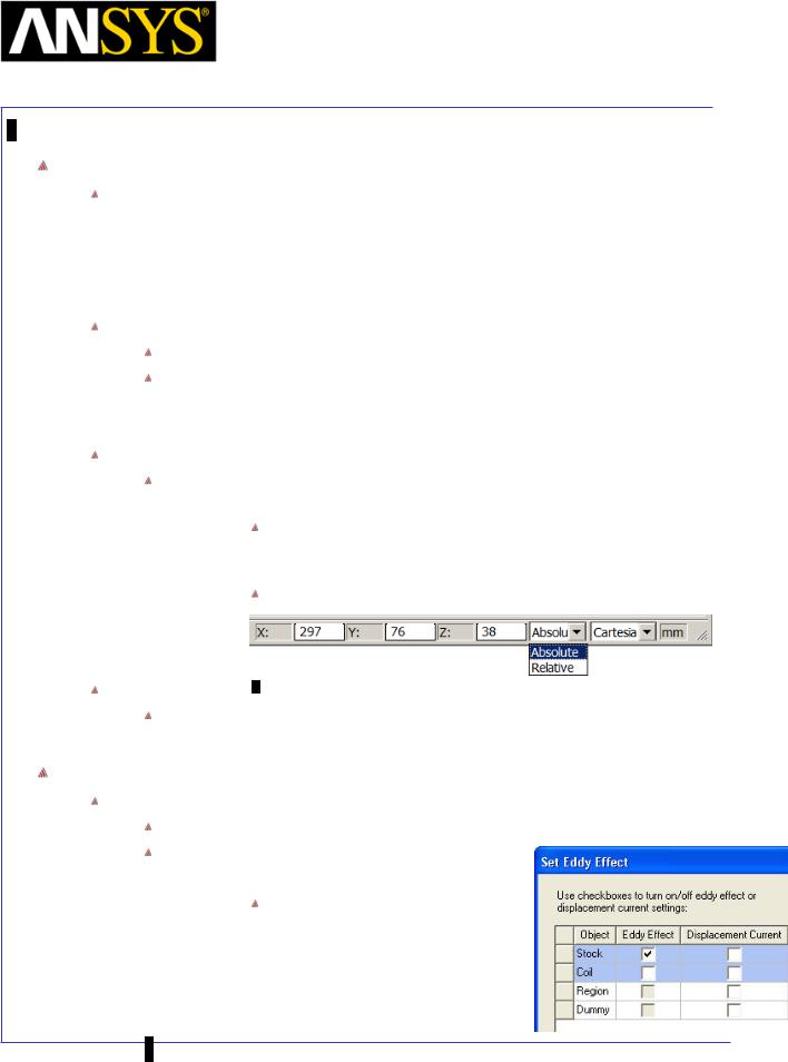
Maxwell v15 |
6.1 |
Example (Eddy Current) – Asymmetric Conductor
Create Dummy Object
Note: As a post-processing results we are interested to calculate the flux density on a line with the following end points: [0; 72; 34] and [288; 72; 34]. In order to get as accurate results as possible, the mesh around the line has to be fine enough. It is generally a good practice to create dummy objects around regions of interest so that the mesh quality can be better controlled in those regions. For this particular problem we create a box around the line of interest.
Change Work Coordinate System
Goto Modeler > Coordinate System > Set Working CS
In Select Coordinate System Window
1.Select Global
2.Press Select
To Create Dummy Object
Select the menu item Draw > Box
1. Using the coordinate entry fields, enter the box position X: -3, Y: 68, Z: 30, Press the Enter key
2.Using the coordinate entry fields, enter the opposite corner of the box: (in Absolute values)
X: 297, Y: 76, Z: 38, Press the Enter key
Change Attributes
Select the resulting object from the tree and goto Properties window 1. Change the name of the object to Dummy
Set Eddy Effects
To Set Eddy Effects
Select the menu item Maxwell 3D > Excitations > Set Eddy Effect
In Set Eddy Effects window 1. Eddy Effects:
Stock: Checked
 Coil: UnChecked 2. Displacement Current:
 Coil and Stock : Unchecked 3. Press OK
|
|
|
|
ANSYS Maxwell 3D Field Simulator v15 User’s Guide |
6.1-11 |
||
|
|
|
|
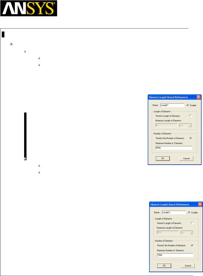
Maxwell v15 |
6.1 |
Example (Eddy Current) – Asymmetric Conductor
Apply Mesh Operations
Apply Length Based Mesh Operations for Dummy
Select the object Dummy from the history tree
Goto menu item Maxwell 3D > Mesh Operations >Assign > Inside Selection
>Length Based
1.Name: Length1
2.Restrict Length of Elements: Unchecked
3.Restrict the Number of Elements: Checked
4.Maximum Number of Elements: 5000
5.Press OK
Apply Length Based Mesh Operations for Stock
Select the object Stock from the history tree
Goto menu item Maxwell 3D > Mesh Operations >Assign > Inside Selection
>Length Based
1.Name: Length2
2.Restrict Length of Elements: Unchecked
3.Restrict the Number of Elements: Checked
4.Maximum Number of Elements: 7500
5.Press OK
|
|
|
|
|
|
|
|
|
|
|
|
|
|
|
|
|
|
|
|
|
|
|
|
|
|
|
|
|
|
|
|
ANSYS Maxwell 3D Field Simulator v15 User’s Guide |
|
6.1-12 |
|||||
|
|
|
|
|
|
|
|
Maxwell v15 |
6.1 |
Example (Eddy Current) – Asymmetric Conductor
Analysis Setup
To create an analysis setup:
Select the menu item Maxwell 3D > Analysis Setup > Add Solution Setup
Solution Setup Window:
1. General Tab
 Percentage Error: 0.2 2. Solver Tab
 Adaptive Frequency: 200 Hz 3. Click the OK button
Save Project
To save the project:
1.In an Ansoft Maxwell window, select the menu item File > Save As.
2.From the Save As window, type the Filename: Ex_6_1_Asymmetrical_Conductor
3.Click the Save button
Model Validation
To validate the model:
Select the menu item Maxwell 3D > Validation Check
Click the Close button
Note: To view any errors or warning messages, use the Message Manager.
Analyze
To start the solution process:
1. Select the menu item Maxwell 3D > Analyze All
ANSYS |
Maxwell 3D Field Simulator v15 User’s Guide |
6.1-13 |
||
|
|
|
|
|

Maxwell v15 |
6.1 |
Example (Eddy Current) – Asymmetric Conductor
Create Objects for Rectangular Plot
To Create Line Object
Select menu item Draw > Line
A massage will pop up asking if the entity needs to be created as non model object. Select Yes to it.
1. Using Co-ordinate entry field Enter the first vertex
X = 0, Y = 72, Z = 34, Press Enter
2. Using Co-ordinate entry field Enter the second vertex
X = 288, Y = 72, Z = 34, Press Enter
Change Attributes
Select the resulting object from the tree and goto Properties window 1. Change the name of the object to FieldLine
Create Parameters
Create parameter Bz_real
Go to Maxwell 3D > Fields > Calculator
1.
2.
3.
4.
Select Input > Quantity > B Select Vector > Scal? > ScalarZ Select General > Complex > Real Select General > Smooth
Note: The flux density will be displayed by default in the units of Tesla [T]. If you wish to see the results in Gaussian units perform steps 5 and 6, otherwise jump to step 7
5. Select Input > Number
6.
7.
Type: Scalar
Value: 10000
Press OK
Select General > *
Select Add and set the name of expression as Bz_real
|
|
|
|
|
|
|
|
|
|
|
|
|
|
|
|
|
|
|
|
|
|
|
|
|
|
|
|
|
|
|
|
|
|
|
|
|
|
|
|
|
|
|
|
|
|
|
|
|
|
|
|
|
|
|
|
|
|
|
|
ANSYS Maxwell 3D Field Simulator v15 User’s Guide |
|
6.1-14 |
|||||||||
|
|
|
|
|
|
|
|
|
|
|
|

Maxwell v15 |
6.1 |
Example (Eddy Current) – Asymmetric Conductor
Create parameter Bz_imag
Go to Maxwell 3D > Fields > Calculator
1.
2.
3.
4.
Select Input > Quantity > B Select Vector > Scal? > ScalarZ Select General > Complex > Imag Select General > Smooth
Note: The flux density will be displayed by default in the units of Tesla [T]. If you wish to see the results in Gaussian units perform steps 5 and 6, otherwise jump to step 7
5. Select Input > Number
6.
7.
8.
Type: Scalar
Value: 10000
Press OK
Select General > *
Select Add and set the name of expression as Bz_imag Press Done
Rectangular Plot
To Create Plot:
Select Maxwell 3D > Results > Create Fields Report > Rectangular Plot
In Reports window
1.Geometry: FieldLine
2.Trace Tab
1.X axis: Default
2.Y axis
Category: Calculator Expressions
Quantity: Bz_real
Function: None
3.Select New Report
4.Without closing window, change quantity to Bz_imag
5.Select Add Trace
6.Select Close
|
|
|
|
|
|
|
|
|
|
|
|
|
|
|
|
|
|
|
|
|
|
|
|
|
|
|
|
|
|
|
|
ANSYS Maxwell 3D Field Simulator v15 User’s Guide |
|
6.1-15 |
|||||
|
|
|
|
|
|
|
|
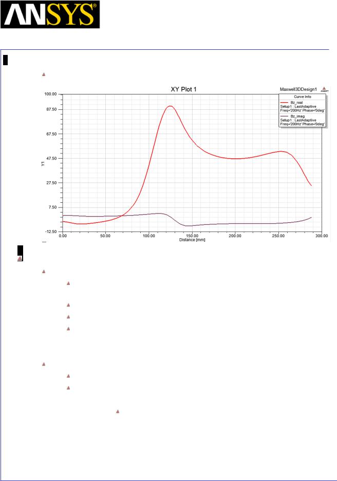
Maxwell v15 |
6.1 |
Example (Eddy Current) – Asymmetric Conductor
Rectangular Plot
Field Overlays
Create Field Plots for Mag_J
Double click on Maxwell3D Design1 from Project Manager window to return to Maxwell Project
Select the object Stock from history tree
Select menu item Maxwell 3D > Fields > Fields > J > Mag_J
In Create Field Plot window
1.Plot on surface only : Checked
2.Select Done
Modify Plot Attributes
Double click on the legend to change plot properties
In the window
1. Scale tab
Num. Divisions: 50
2. Press Apply and Close
|
|
|
|
|
|
|
|
|
|
|
|
|
|
|
|
|
|
|
|
|
|
|
|
|
|
|
|
|
|
|
|
|
|
|
|
|
|
|
|
|
|
|
|
|
|
|
|
|
|
|
|
|
|
|
|
|
|
|
|
ANSYS Maxwell 3D Field Simulator v15 User’s Guide |
|
6.1-16 |
|||||||
|
|
|
|
|
|
|
|
|
|
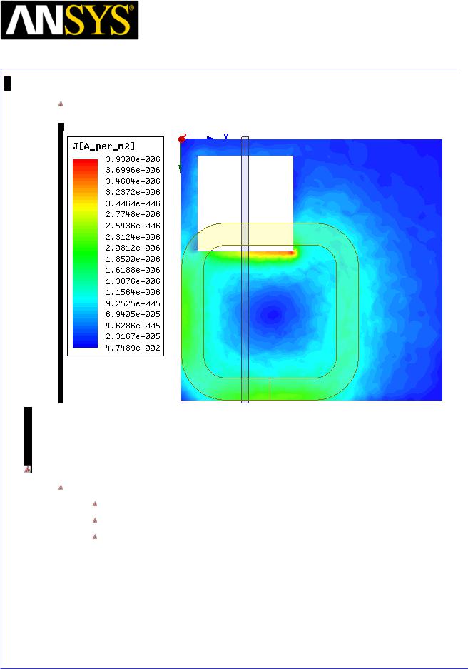
Maxwell v15 |
6.1 |
Example (Eddy Current) – Asymmetric Conductor
Field Plots Mag_J
Vector Plot
Create Vector Plot
Select the object Stock from history tree
Select menu item Maxwell 3D > Fields > Fields > J > Vector_J
In Create Field Plot window
1.In Volume: AllObjects
2.Plot on surface only : Checked
3.Select Done
|
|
|
|
|
|
|
|
|
|
|
|
ANSYS Maxwell 3D Field Simulator v15 User’s Guide |
|
6.1-17 |
|||
|
|
|
|
|
|
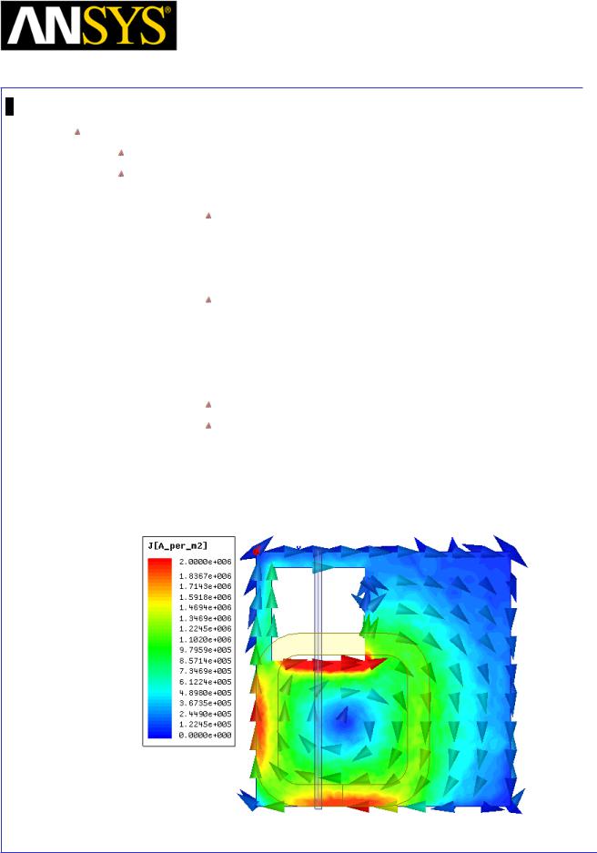
Maxwell v15 |
6.1 |
Example (Eddy Current) – Asymmetric Conductor
Modify Plot Attributes
Double click on the legend to change plot properties
In the window 1. Scale tab
User Limits: Checked
1.Min: 0
2.Max: 2e6
2.Marker/Arrow tab
Arrow Options
1.Size: Set to appropriate value
2.Map Size: Unchecked
3.Arrow tail: Unchecked
3. Plots tab
Plot: Vector_J1
Vector Plot
1.Spacing: Set to Minimum
2.Min: 30
3.Max: 60
4.Press Apply and Close
|
|
|
|
|
|
|
|
|
|
|
|
|
|
|
|
|
|
|
|
|
|
|
|
|
|
|
|
|
|
|
|
ANSYS Maxwell 3D Field Simulator v15 User’s Guide |
|
6.1-18 |
|||||
|
|
|
|
|
|
|
|
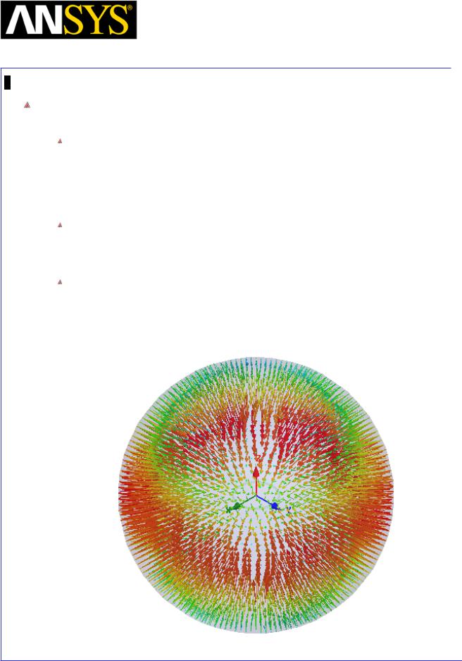
Maxwell v15 |
6.2 |
Example (Eddy Current) – Radiation Boundary
The implementation and application of a Radiation Boundary in the Eddy Current Solver
Radiation Boundaries are used when one wants to simulate the free emission of fields into space. The main distinction of this boundary from all other boundary conditions is that the radiation boundary does not enforce any restrictions on the field behavior. This is used specifically to model unbounded eddy currents and propagating waves without reflection. This boundary has several specific uses which will be discussed in detail in this document.
Note that Maxwell3D is a low-frequency simulator, so it is not recommended to model standard antennas and wave propagation with this tool. Maxwell is ideal for near-field simulations for the investigation of interactions between lowfrequency inductors and RFID applications.
The example that will be used to demonstrate how Radiation Boundaries are implemented is a Magnetic Dipole. The intent of this write up is not how to simulate a dipole antenna, it is rather to demonstrate how Radiation Boundaries are implemented within the Eddy Current solver.
|
|
|
|
|
|
|
|
|
|
|
|
|
|
|
|
|
|
|
|
|
|
|
|
|
|
|
|
|
|
|
|
ANSYS Maxwell 3D Field Simulator v15 User’s Guide |
|
6.2-1 |
|||||
|
|
|
|
|
|
|
|

Maxwell v15 |
6.2 |
Example (Eddy Current) – Radiation Boundary
ANSYS Maxwell Design Environment
The following features of the ANSYS Maxwell Design Environment are used to
create the models covered in this topic
3D Solid Modeling
Primitives: Torus, Sphere
Surface Operations: Section
Boolean Operations: Separate Bodies
Boundaries/Excitations
Current: Solid
Radiation Boundary
Symmetry Boundary
Analysis
Eddy Current
Results
Calculator Expressions
Field Overlays:
Field Plots
|
|
|
|
|
|
|
|
|
|
|
|
|
|
|
|
|
|
|
|
|
|
|
|
|
|
|
|
|
|
|
|
ANSYS Maxwell 3D Field Simulator v15 User’s Guide |
|
6.2-2 |
|||||
|
|
|
|
|
|
|
|

Maxwell v15 |
6.2 |
Example (Eddy Current) – Radiation Boundary
Launching Maxwell
To access Maxwell:
1.Click the Microsoft Start button, select Programs, and select Ansoft > Maxwell 15.0 and select Maxwell 15.0
Setting Tool Options
To set the tool options:
Note: In order to follow the steps outlined in this example, verify that the following tool options are set :
1. Select the menu item Tools > Options > Maxwell 3D Options
Maxwell Options Window:
1. Click the General Options tab
Use Wizards for data input when creating new boundaries: Checked
Duplicate boundaries/mesh operations with geometry:
Checked
2.Click the OK button
2.Select the menu item Tools > Options > Modeler Options.
Modeler Options Window:
1. Click the Operation tab
 Automatically cover closed polylines: Checked 2. Click the Display tab
 Default transparency = 0.8 3. Click the Drawing tab
 Edit property of new primitives: Checked 4. Click the OK button
|
|
|
|
|
|
|
|
|
|
|
|
|
|
|
|
|
|
|
|
|
|
|
|
|
|
|
|
|
|
|
|
ANSYS Maxwell 3D Field Simulator v15 User’s Guide |
|
6.2-3 |
|||||
|
|
|
|
|
|
|
|

Maxwell v15 |
6.2 |
Example (Eddy Current) – Radiation Boundary
Opening a New Project
To open a new project:
After launching Maxwell, a project will be automatically created. You can also create a new project using below options.
1.In an Maxwell window, click the On the Standard toolbar, or select the menu item File > New.
Select the menu item Project > Insert Maxwell 3D Design, or click on the icon
Set Solution Type
To set the Solution Type:
Select the menu item Maxwell 3D > Solution Type
Solution Type Window:
1.Choose Eddy Current
2.Click the OK button
|
|
|
|
|
|
|
|
|
|
|
|
|
|
|
|
|
|
|
|
|
|
|
|
|
|
|
|
|
|
|
|
|
|
|
|
|
|
|
|
|
|
|
|
|
|
|
|
|
|
|
|
|
|
|
|
|
|
|
|
ANSYS Maxwell 3D Field Simulator v15 User’s Guide |
|
6.2-4 |
|||||||
|
|
|
|
|
|
|
|
|
|
Maxwell v15 |
6.2 |
Example (Eddy Current) – Radiation Boundary
Set Model Units
To Set the units:
Select the menu item Modeler > Units
Set Model Units:
1.Select Units: meter
2.Click the OK button
Set Default Material
To set the default material:
Using the 3D Modeler Materials toolbar, choose Select
In Select Definition window,
1.Type copper in the Search by Name field
2.Click the OK button
|
|
|
|
|
|
|
|
|
|
|
|
|
|
|
|
|
|
|
|
|
|
|
|
|
|
|
|
|
|
|
|
ANSYS Maxwell 3D Field Simulator v15 User’s Guide |
|
6.2-5 |
|||||
|
|
|
|
|
|
|
|

|
|
|
Maxwell v15 |
|
6.2 |
|
|
Example (Eddy Current) – Radiation Boundary |
|
||
|
|
|
|
||
|
|
Create Dipole Ring |
|
||
|
|
|
|||
|
|
|
|||
|
|
Create Torus |
|
||
|
|
Select the menu item Draw > Torus |
|
||
1. |
Using the coordinate entry fields, enter the center point of torus |
||||
|
|
|
X: 0, Y: 0, Z: 0, Press the Enter key |
|
|
2. |
Using the coordinate entry fields, enter the inner radius |
|
|||
|
|
|
dX: 0.0095, dY: 0, dZ: 0, Press the Enter key |
|
|
3. |
Using the coordinate entry fields, enter the outer radius |
|
|||
|
|
|
dX: 0.001, dY: 0, dZ: 0, Press the Enter key |
|
|
|
|
Select the menu item View > Fit All > Active View. |
|
||
|
|
Change Attributes |
|
||
|
|
Select the resulting object from the tree and goto Properties window |
|
||
1. |
Change the name of the object to Ring |
|
|||
2. |
Change its color to Green |
|
|||
Create Excitations
Create Section of coil for assigning Current
Select the object Ring from the history tree
Select the menu item Modeler > Surface > Section
In Section window,
1.Section Plane: YZ
2.Click the OK button
Change Attributes
Select the object Ring_Section1 from the tree and goto Properties window 1. Change the name of the object to Terminal
Separate Sheets
Select the sheet Terminal
Select the menu item Modeler > Boolean > Separate Bodies
Delete Extra Sheets
Select the sheet Terminal_Seperate1 from the tree Select the menu item Edit >Delete
|
|
|
|
|
|
|
|
|
|
|
|
|
|
|
|
|
|
|
|
|
|
|
|
|
|
|
|
|
|
|
|
|
|
|
|
|
|
|
|
|
|
|
|
|
|
|
|
|
|
|
|
|
|
6.2-6 |
|||||
ANSYS Maxwell 3D Field Simulator v15 User’s Guide |
|
|
|||||||
|
|
|
|
|
|
|
|
|
|
Maxwell v15 |
6.2 |
Example (Eddy Current) – Radiation Boundary
Assign Excitations
Select the sheet Terminal from the history tree
Select the menu item Maxwell 3D > Excitations > Assign > Current
In Current Excitation window,
1.Name: Current1
2.Value: 1.414
3.Phase: 0
4.Type: Solid
6. Press OK
Note: In Eddy Current Solver, peak current is always specified instead of RMS
Set Default Material
To Set Default Material
Using the 3D Modeler Materials toolbar, choose Vacuum
Create Region
To create the region:
Select the menu item Draw > Sphere
1. Using the coordinate entry fields, enter the center of Sphere
X: 0, Y: 0, Z: 0, Press the Enter key
2. Using the coordinate entry fields, enter the radius:
dX: 0.06 dY: 0, dZ: 0, Press the Enter key
Change Attributes
Select the resulting object from the tree and goto Properties window 1. Change the name of the object to Region
|
|
|
|
|
|
|
|
|
|
|
|
ANSYS Maxwell 3D Field Simulator v15 User’s Guide |
|
6.2-7 |
|||
|
|
|
|
|
|
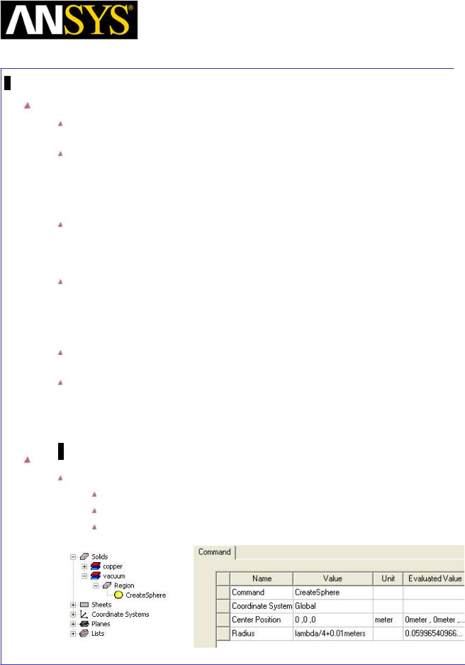
Maxwell v15 |
6.2 |
Example (Eddy Current) – Radiation Boundary
Radiation Boundary Overview
The radiation boundary is only available in the Eddy Current solver – it is only applicable for frequency domain solutions.
The radiation boundary should be used in conjunction with displacement current in the background object – implying that the fields in the background can propagate to the edge of the model. This means that if displacement currents are simulated in the background, then a radiation boundary should be used on the outside surface of the background.
A radiation boundary is used to simulate an open problem that allows waves to radiate infinitely far into space, such as antenna designs. Maxwell3D absorbs the wave at the radiation boundary, essentially ballooning the boundary infinitely far away from the structure.
A radiation surface does not have to be spherical, but it must be exposed to the background, convex with regard to the radiation source, and located at least a quarter wavelength from the radiating source. In some cases the radiation boundary may be located closer than one-quarter wavelength, such as portions of the radiation boundary where little radiated energy is expected.
Remember that Maxwell3D is a near-field simulator, so the dimension of components should be much smaller than the wavelength (i.e. lambda/10)
The wavelength at 1.5GHz is 0.2m. Therefore, our 0.06m radius sphere is more than one quarter wavelength from the ring. In order to make the boundary placement more automated, we can use variables and equations to define the size of the bounding object.
Assign Function to the Radius of the Region
Specify Radius of Region as Function of Speed of Light “c0” and Frequency
Expand the history tree of the object Region
Double click on the command CreateSphere from the tree For Radius, type: lambda/4 + 0.01meters, Click the Tab key
|
|
|
|
|
|
|
|
|
|
|
|
|
|
|
|
|
|
|
|
|
|
|
|
|
|
|
|
|
|
|
|
ANSYS Maxwell 3D Field Simulator v15 User’s Guide |
|
6.2-8 |
|||||
|
|
|
|
|
|
|
|
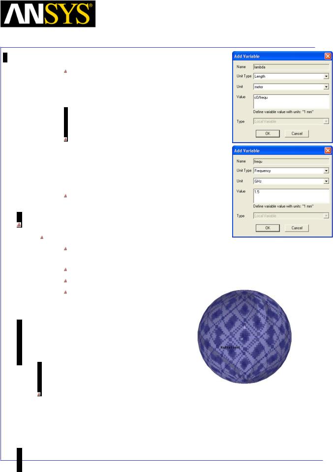
Maxwell v15 |
6.2 |
Example (Eddy Current) – Radiation Boundary
In Add variable window for lambda
1.Value: c0/frequ
2.Press OK
In Add variable window for frequ
1.Unit Type: Frequency
2.Unit: GHz
3.Value: 1.5
4.Press OK
Press OK
Assign Boundary
Assign Radiation Boundary
Select the menu item Edit > Select > Faces or press F from the keyboard to change selection to faces
Select the face of the Region
Select the menu item Maxwell 3D > Boundaries > Assign > Radiation
In Radiation Boundary window, 1. Press OK
Note: This assigns a radiation boundary to the outside of the sphere, allowing the waves to propagate outside of the sphere. If no radiation boundary is assigned, the interactions of the components may be correct, but the fields near the boundaries will certainly be incorrect. The Poynting vector on the outer surface is a clear indicator of this, which we will explore later.
|
|
|
|
|
|
|
|
|
|
|
|
|
|
ANSYS |
Maxwell 3D Field Simulator v15 User’s Guide |
|
6.2-9 |
|||
|
|
|
|
|
|
|
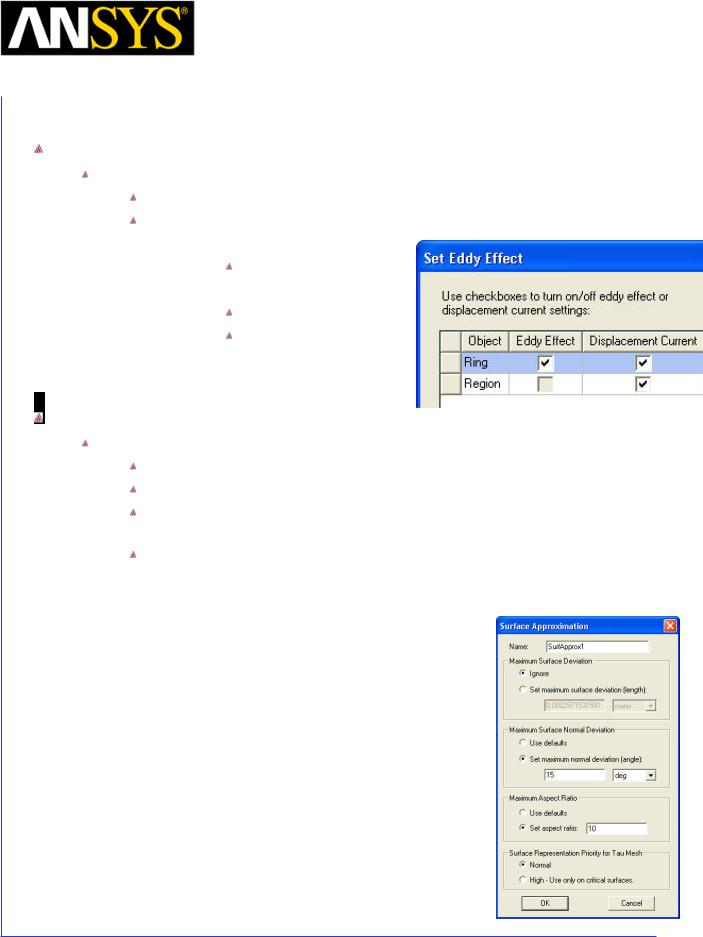
|
|
|
Maxwell v15 |
|
6.2 |
|
|
Example (Eddy Current) – Radiation Boundary |
|
||
|
|
|
|
||
|
|
Set Eddy Effects |
|
||
|
|
|
|||
|
|
|
|||
|
|
To Set Eddy Effects |
|
||
|
|
Select the menu item Maxwell 3D > Excitations > Set Eddy Effect |
|
||
|
|
In Set Eddy Effects window |
|
||
1. |
Eddy Effects: |
|
|||
|
|
|
Ring: Checked |
|
|
2. |
Displacement Current: |
|
|||
|
|
|
Ring: Checked |
|
|
|
|
|
Region: Checked |
|
|
3. |
Press OK |
|
|||
Apply Mesh Operations
Apply Length Based Mesh Operations for Ring
Select the menu item Edit >Select > Objects or press “O” from keyboard
Select the object Ring from the history tree
Goto menu item Maxwell 3D > Mesh Operations >Assign > Surface Approximation
In Surface Approximation window
1. Maximum Surface Normal Deviation
 Set maximum normal deviation (angle): 15 deg 2. Maximum Aspect Ratio
 Set Aspect Ratio: 10 3. Press OK
|
|
|
|
|
|
|
|
|
|
|
|
|
|
|
|
|
|
|
|
|
|
|
|
|
|
|
|
|
|
|
|
|
|
|
|
|
|
|
|
|
|
|
|
|
|
|
|
|
|
|
|
|
|
|
|
|
|
|
|
ANSYS Maxwell 3D Field Simulator v15 User’s Guide |
|
6.2-10 |
|||||||
|
|
|
|
|
|
|
|
|
|
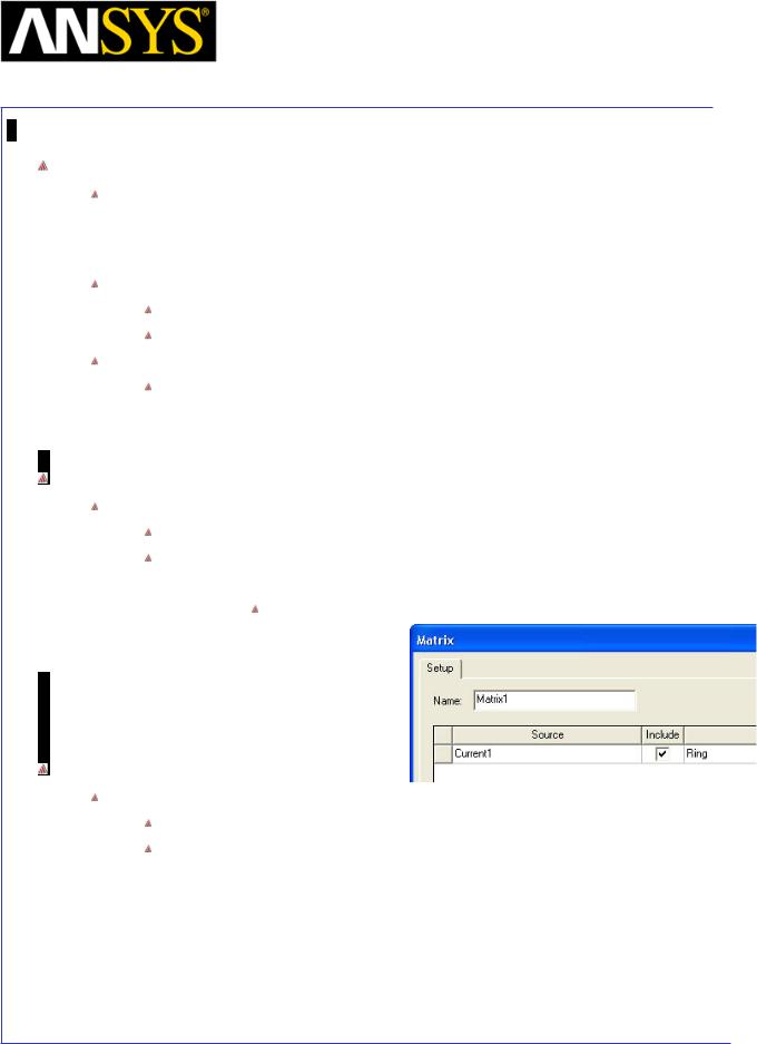
Maxwell v15 |
6.2 |
Example (Eddy Current) – Radiation Boundary
Create Outer Surface
Note: One important part of creating a geometry is to consider the results needed in the post-processor. We will wish to use the outer surface of the sphere to compute the radiated power and the radiation resistance. Therefore, we will need to create a surface to integrate over that defines precisely the area that we need.
To Create Outer Surface
Select the outer face of the Region
Select the menu item Modeler > Surface > Create Object from Face
Change Attributes
Select the resulting object from the tree and goto Properties window 1. Change the name of the object to Outside
Assign Matrix Parameters
To Assign Parameters
Select the menu item Maxwell 3D > Parameters > Assign > Matrix
In Matrix window
1. Current1
Include: Checked
2. Press OK
Analysis Setup
To create an analysis setup:
Select the menu item Maxwell 3D > Analysis Setup > Add Solution Setup
Solution Setup Window:
1. General Tab
 Percentage Error: 0.2 2. Solver Tab
 Adaptive Frequency: 1.5 GHz 3. Click the OK button
|
|
|
|
|
|
|
|
|
|
|
|
|
|
|
|
ANSYS Maxwell 3D Field Simulator v15 User’s Guide |
|
6.2-11 |
|||||
|
|
|
|
|
|
|
|
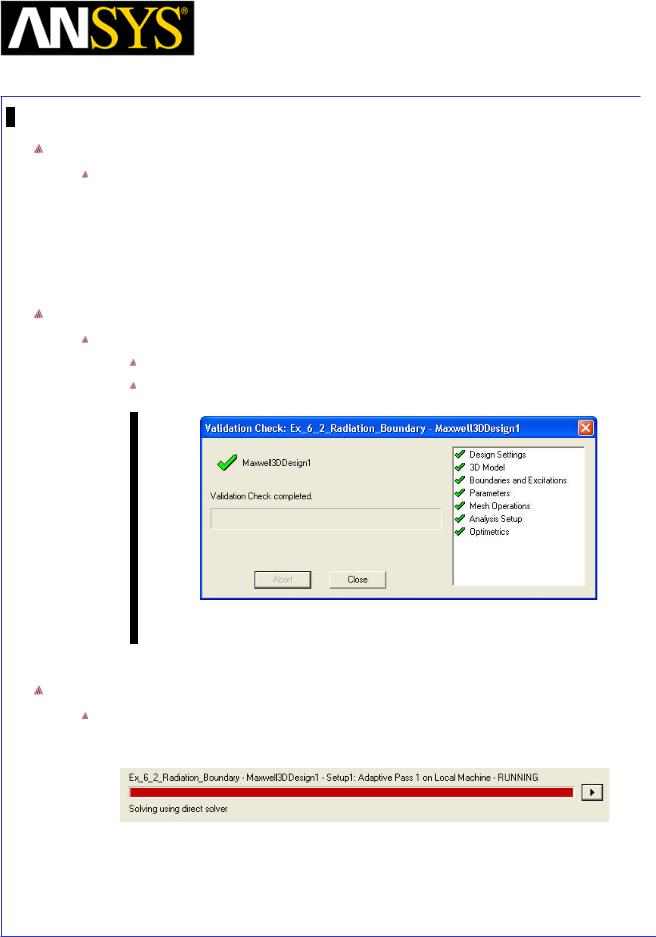
Maxwell v15 |
6.2 |
Example (Eddy Current) – Radiation Boundary
Save Project
To save the project:
1.In an Ansoft Maxwell window, select the menu item File > Save As.
2.From the Save As window, type the Filename: Ex_6_2_Radiation_Boundary
3.Click the Save button
Model Validation
To validate the model:
Select the menu item Maxwell 3D > Validation Check
Click the Close button
Note: To view any errors or warning messages, use the Message Manager.
Analyze
To start the solution process:
1. Select the menu item Maxwell 3D > Analyze All
|
|
|
|
|
|
|
|
|
|
|
|
|
|
|
|
|
|
|
|
|
|
|
|
|
|
|
|
|
|
|
|
ANSYS Maxwell 3D Field Simulator v15 User’s Guide |
|
6.2-12 |
|||||
|
|
|
|
|
|
|
|
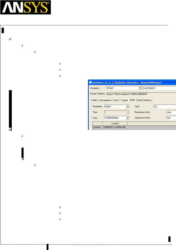
Maxwell v15 |
6.2 |
Example (Eddy Current) – Radiation Boundary
Solution Data
To view the Solution Data:
Select the menu item Maxwell 3D > Results > Solution Data
1. To view Impedance Matrix
Select the Matrix tab
Set Parameter to Matrix1 Set Type to R,L
2. Press Close
Create Parameters
Note: We will create a Poynting vector expression in the calculator that is
accessible as a field plot and for power calculations. The expression will be:
P = 12 Re{E ×H }
Create parameter Poynting
Goto Maxwell 3D > Fileds > Calculator
1.Select Input > Quantity > E
2.Select Input > Quantity > H
3.Select General > Complex > Conj
4.Select Vector > Cross
5.Select General > Complex > Real
6.Select Input > Number
Type: Scalar
Value: 0.5
Press OK
6.Select General > *
7.Select Add and set the name of expression as Poynting
8.Press Done
ANSYS Maxwell 3D Field Simulator v15 User’s Guide |
6.2-13 |
||||
|
|
|
|
|
|
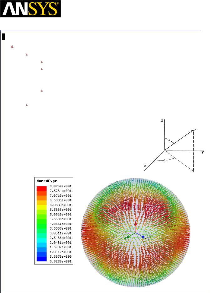
Maxwell v15 |
6.2 |
Example (Eddy Current) – Radiation Boundary
Create Vector Plot
To Create Vector Plot
Select outer surface of the object Region
Select the menu item Maxwell 3D > Fields > Fields > Named Expressions
1.Select the parameter Poynting
2.Press OK
In Create Field Plot window 1. Press Done
A plot similar to the following should appear, with strong fields near theta=90°.
|
|
|
|
|
|
|
|
|
|
|
|
|
|
|
|
|
|
|
|
|
|
|
|
|
|
|
|
|
|
|
|
|
|
|
|
|
|
|
|
|
|
|
|
|
|
|
|
|
|
|
|
|
|
|
|
|
|
|
|
ANSYS Maxwell 3D Field Simulator v15 User’s Guide |
|
6.2-14 |
|||||||
|
|
|
|
|
|
|
|
|
|
Maxwell v15 |
6.2 |
Example (Eddy Current) – Radiation Boundary
Calculate the Radiation Resistance
Note:
The radiation resistance of an antenna is determined by the following
formula: |
Pav |
R = |
|
r |
Irms2 |
|
Where the radiated Power is defined as the integral of the Poynting vector
over the surface S (outer surface of the region).
Pav = 1 ∫∫Re(E ×H * )dS
2 S
Since the rms current is 1 A (the peak current is defined as 1.414 A), the radiation resistance is simply the result of this integral.
To Calculate Radiated Power
Goto Maxwell 3D > Fileds > Calculator
1.
2.
3.
4.
5.
6.
Select Poynting from Named Expressions list Select Copy to Stack
Select Input > Geometry
Select Surface
Select Outside from the list
 Press OK Select Vector > Normal
Select Scalar >  (Integrate) Press Eval
The resulting value should be around -2.165 W
Since RMS current comes out to be 1A, the radiation resistance should also be -2.165 Ohms
Note:
According to the literature, the radiation resistance of a Magnetic Dipole with no thickness is:
Rrad _ air = 20π2β4a4
where β is the wave number and a is the radius of the loop
This equation results in 1.923 ohms for a radius of 0.01m and a wavelength of 0.2m. 
ANSYS Maxwell 3D Field Simulator v15 User’s Guide |
6.2-15 |
||
|
|
|
|
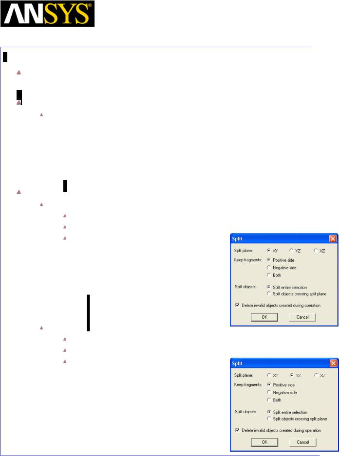
Maxwell v15 |
6.2 |
Example (Eddy Current) – Radiation Boundary
PART 2: Create a 1/16th Section Model
Create Symmetry Design
Copy Design
1.Select the design Maxwell3D Design1 in Project Manager window, right click and select Copy
2.Select project Ex_6_2_Radiation_Boundary in Project Manager window and select Paste
3.Change the name of the design to 1_16_Model
Split Model for 1/16th Section
Divide by XY Plane
Select the menu item Edit > Select All
Select the menu item Modeler > Boolean >Split
In Split window
1.Split plane: XY
2.Keep fragments: Positive side
3.Split objects: Split entire selection
4.Press OK
Divide by YZ Plane
Select the menu item Edit > Select All
Select the menu item Modeler > Boolean >Split
In Split window
1.Split plane: YZ
2.Keep fragments: Positive side
3.Split objects: Split entire selection
4.Press OK
|
|
|
|
|
|
|
|
|
|
|
|
|
|
|
|
|
|
|
|
|
|
|
|
|
|
|
|
|
|
|
|
ANSYS Maxwell 3D Field Simulator v15 User’s Guide |
|
6.2-16 |
|||||
|
|
|
|
|
|
|
|
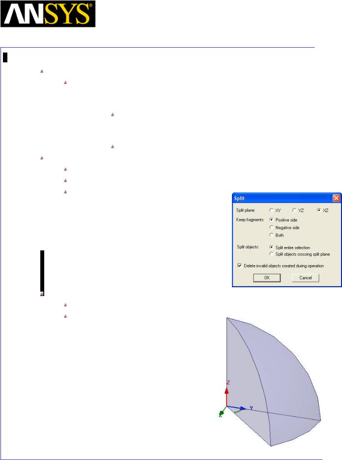
Maxwell v15 |
6.2 |
Example (Eddy Current) – Radiation Boundary
Create Relative Coordinate System
Select the menu item Modeler > Coordinate System > Create > Relative CS > Rotated
1. Using the coordinate entry field, enter the X axis position X: 0.01, Y: 0.01, Z: 0, Press the Enter key
2.Using the coordinate entry field, enter the XY Plane position in Absolute values
X: -0.01, Y: 0.01, Z: 0, Press the Enter key
Divide by XZ Plane
Select the menu item Edit > Select All
Select the menu item Modeler > Boolean >Split
In Split window
1.Split plane: XZ
2.Keep fragments: Positive side
3.Split objects: Split entire selection
4.Press OK
Change Work Coordinate System
Goto Modeler > Coordinate System > Set Working CS
In Select Coordinate System Window
1.Select Global
2.Press Select
|
|
|
|
|
|
|
|
|
|
|
|
ANSYS Maxwell 3D Field Simulator v15 User’s Guide |
|
6.2-17 |
|||
|
|
|
|
|
|
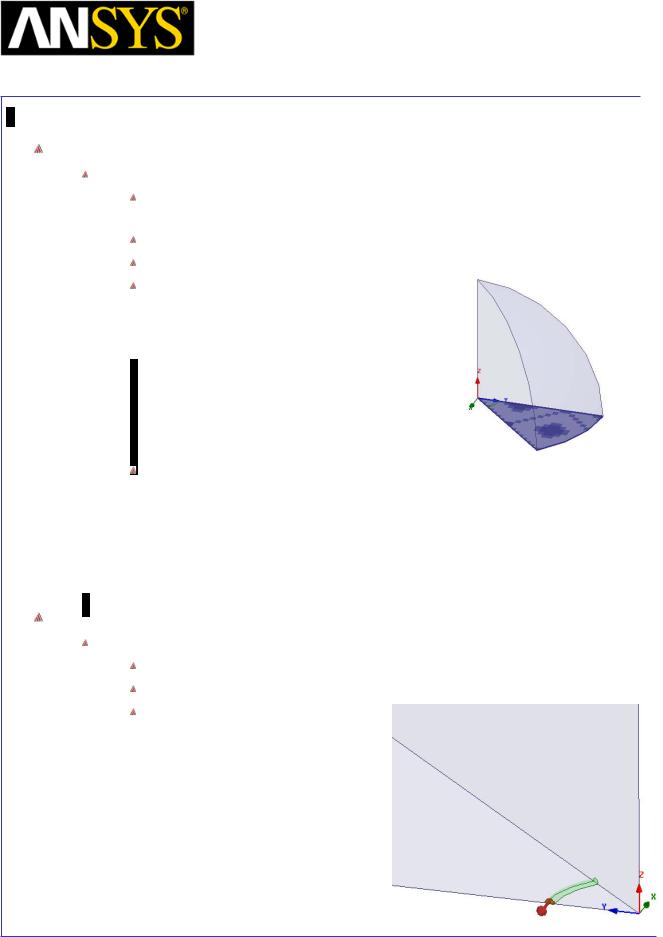
Maxwell v15 |
6.2 |
Example (Eddy Current) – Radiation Boundary
Assign Boundaries
To Assign Symmetry Boundaries
Select the menu item Edit > Select > Faces or press F from the keyboard to change selection to faces
Select the face of the Region with which touch with XY Plane
Select the menu item Maxwell 3D > Boundaries > Assign > Symmetry
In Symmetry Boundary window,
1.Symmetry: Even (Flux Normal)
2.Press OK
Note: Only one symmetry boundary is required even though three surfaces define distinct symmetries. The two surfaces perpendicular to the ring have a symmetry that is accounted for by the default boundary condition of Zero Tangential H Field – i.e. this is a special case of symmetry, where the symmetric tangential fields are zero. The surface that lies in the plane of the ring has a Flux Normal symmetry, so we need to define this separately.
Create Excitations
Assign Excitation Current_Out
Select the face of Ring which touches the YZ Plane
Select the menu item Maxwell 3D > Excitations > Assign >Current
In Current Excitation window,
1.Name: Current_Out
2.Value: 0.707 A
3.Type: Solid
4.Direction: Out of Model
5.Press OK
|
|
|
|
|
|
|
|
|
|
|
|
ANSYS Maxwell 3D Field Simulator v15 User’s Guide |
|
6.2-18 |
|||
|
|
|
|
|
|
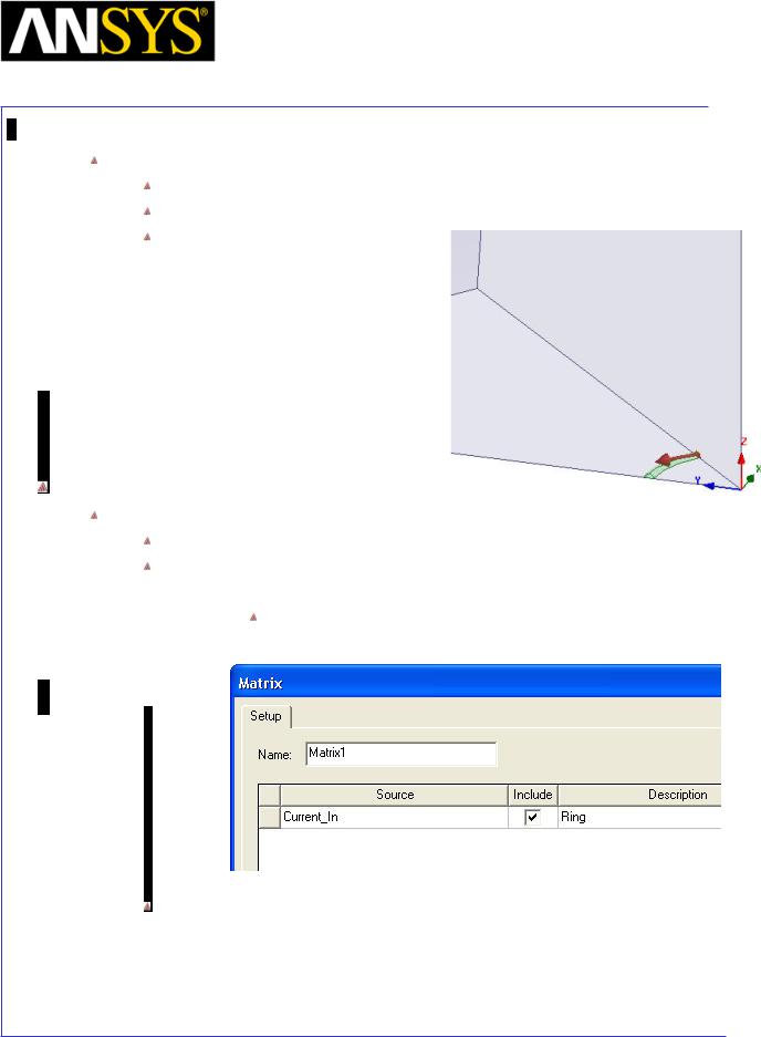
Maxwell v15 |
6.2 |
Example (Eddy Current) – Radiation Boundary
Assign Excitation Current_In
Select the face of Ring as shown in image
Select the menu item Maxwell 3D > Excitations > Assign >Current
In Current Excitation window,
1.Name: Current_In
2.Value: 0.707 A
3.Type: Solid
4.Direction: Going in to Model
5.Press OK
Assign Matrix Parameters
To Assign Parameters
Select the menu item Maxwell 3D > Parameters > Assign > Matrix
In Matrix window
1. Current_In
Include: Checked
2. Press OK
Note: The excitations available to the Matrix are only those excitations that define the current entering the conduction path. The Current_Out excitation defines current exiting the conduction path, and so is not available to the matrix.
|
|
|
|
|
|
|
|
|
|
|
|
ANSYS Maxwell 3D Field Simulator v15 User’s Guide |
|
6.2-19 |
|||
|
|
|
|
|
|
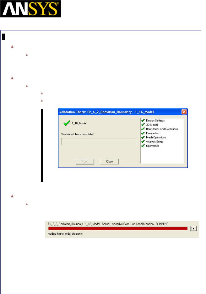
Maxwell v15 |
6.2 |
Example (Eddy Current) – Radiation Boundary
Save Project
To save the project:
1. In an Ansoft Maxwell window, select the menu item File > Save
Model Validation
To validate the model:
Select the menu item Maxwell 3D > Validation Check
Click the Close button
Note: To view any errors or warning messages, use the Message Manager.
Analyze
To start the solution process:
1. Select the menu item Maxwell 3D > Analyze All
|
|
|
|
|
|
|
|
|
|
|
|
|
|
|
|
|
|
|
|
|
|
|
|
|
|
|
|
|
|
|
|
ANSYS Maxwell 3D Field Simulator v15 User’s Guide |
|
6.2-20 |
|||||
|
|
|
|
|
|
|
|
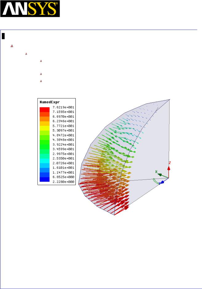
Maxwell v15 |
6.2 |
Example (Eddy Current) – Radiation Boundary
Plot Power Flow
To View vector Plot
In the Project Manager tree, expand Field Overlays and NamedExpr to find Poynting1
Double click on Poyntning1 to refresh the plot The plot should look similar to the following
|
|
|
|
|
|
|
|
|
|
|
|
|
|
|
|
|
|
|
|
|
|
|
|
|
|
|
|
|
|
|
|
|
|
|
|
|
|
|
|
|
|
|
|
|
|
|
|
|
|
|
|
|
|
|
|
|
|
|
|
ANSYS Maxwell 3D Field Simulator v15 User’s Guide |
|
6.2-21 |
|||||||
|
|
|
|
|
|
|
|
|
|
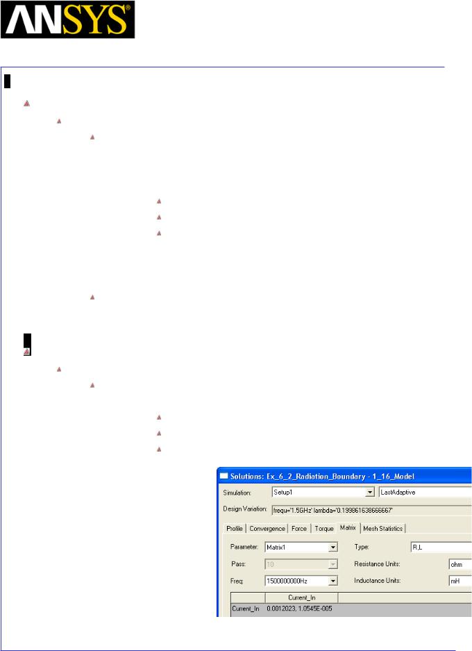
Maxwell v15 |
6.2 |
Example (Eddy Current) – Radiation Boundary
Calculate the Radiation Resistance
To Calculate Radiated Power
Goto Maxwell 3D > Fileds > Calculator
1.Select Poynting from Named Expressions list
2.Select Copy to Stack
3.Select Input > Geometry
Select Surface
Select Outside from the list
Press OK
4.Select Vector > Normal
5.Select Scalar >  (Integrate)
6.Press Eval
The resulting value should be around -0.1336 W which is around 1/16th of previous value
Solution Data
To view the Solution Data:
Select the menu item Maxwell 3D > Results > Solution Data
1. To view Impedance Matrix
Select the Matrix tab
Set Parameter to Matrix1 Set Type to R,L
2. Press Close
|
|
|
|
|
|
|
|
|
|
|
|
|
|
|
|
|
|
|
|
|
|
|
|
|
|
|
|
|
|
|
|
ANSYS Maxwell 3D Field Simulator v15 User’s Guide |
|
6.2-22 |
|||||
|
|
|
|
|
|
|
|