


Maxwell Overview Presentation
v15 3.3
Maxwell and the Finite Element Method
Maxwell uses the Finite Element Method (FEM) to solve Maxwell‘s equations. The primary advantage of the FEM for solving partial differential equations lies in the ability of the basic building blocks used to discretize the model to conform to arbitrary geometry.
The arbitrary shape of the basic building block (tetrahedron) also allows Maxwell to generate a coarse mesh where fewer cells are needed to yield an accurate solution, while creating a finely discretized mesh where the field is rapidly varying or higher accuracy is needed to obtain an accurate global solution.
The FEM has been a standard for solving electromagnetic problems since the 1970s. Maxwell appeared on the market in 1984 pioneering the use of adaptive meshing in a commercial product.
The FEM has been a standard for solving problems in structure mechanics since the mid 1950‘s (imagine defining the 3D structure of a bridge with punch cards)!
First see the one-dimensional example…..
ANSYS Maxwell Field Simulator v15 – Training Seminar |
3.3-2 |
|
|
Maxwell v15 |
Overview |
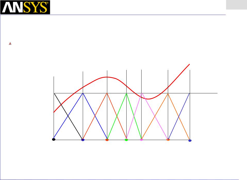
The Finite Element Method in 1-D
The finite element method (FEM) can be used to approximate the unknown curve F(x)
w |
w2 |
w3 |
w4 |
w5 |
w6 |
F(x) 0 |
w1 |
|
|
|
|
1 |
|
|
|
|
|
|
|
|
|
|
0 |
|
|
|
|
6x |
1 |
2 |
3 |
4 |
5 |
The model is “discretized into 6 individual cells. w0 – w6 are the piecewise linear “basis functions” from which the approximate solution will be built.
Presentation
3.3
ANSYS Maxwell Field Simulator v15 – Training Seminar |
3.3-3 |
|
|
Maxwell v15 |
Overview |
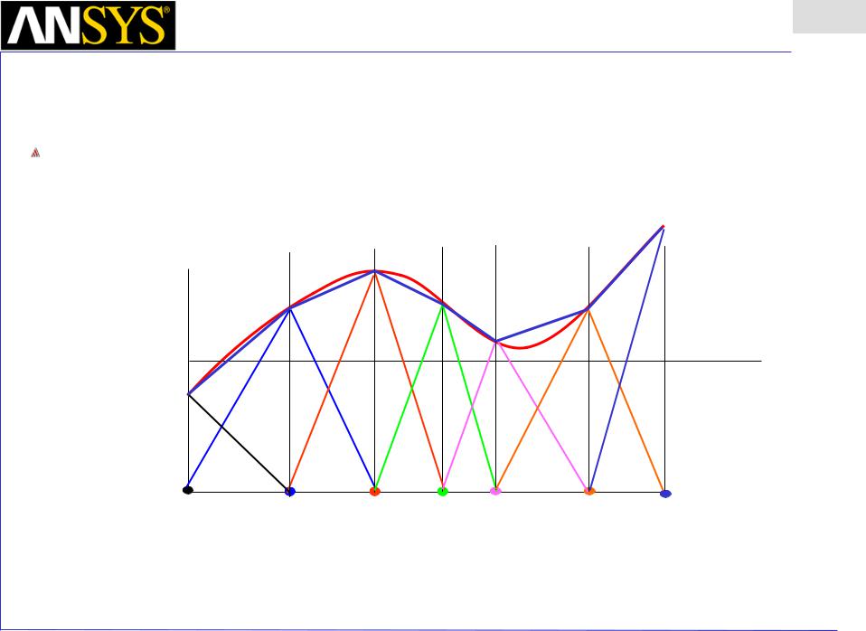
The Finite Element Method in 1-D
In the FEM, the unknown function is expressed as a weighted sum of the piecewise continuous basis functions.
F’(x)=Σai wi
F(x)
1
Node 1 |
2 |
3 |
4 |
5 |
6x |
The approximate solution resulting from the FEM calculation is F’(x) shown as a dotted line.
Presentation
3.3
ANSYS Maxwell Field Simulator v15 – Training Seminar |
3.3-4 |
|
|
Maxwell Overview Presentation
v15 3.3
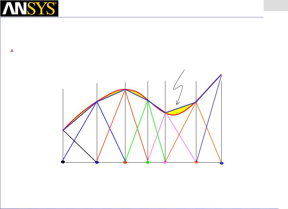
The Finite Element Method in 1-D
A key feature of the FEM as it is implemented in Maxwell is the ability to locally determine the error. Recall that F(x) is not known, but the ERROR can be determined1. Error!
Node 1 |
2 |
3 |
4 |
5 |
6x |
1Cendes, Z.J., and D.N. Shenton. Adaptive mesh refinement in the finite element. computation of magnetic fields; IEEE Transactions on magnetics (T-MAG), Pages 1811-1816 , Volume 21, Issue 5, Sept 1985
ANSYS Maxwell Field Simulator v15 – Training Seminar |
3.3-5 |
|
|