

Maxwell v15 Overview
Presentation
1
Maxwell 3D Keyboard Shortcuts
General Shortcuts
•F1: Help
•Shift + F1: Context help
•CTRL + F4: Close program
•CTRL + C: Copy
•CTRL + N: New project
•CTRL + O: Open...
•CTRL + S: Save
•CTRL + P: Print...
•CTRL + V: Paste
•CTRL + X: Cut
•CTRL + Y: Redo
•CTRL + Z: Undo
•CTRL + 0: Cascade windows
•CTRL + 1: Tile windows horizontally
•CTRL + 2: Tile windows vertically
Modeller Shortcuts
•B: Select face/object behind current selection
•F: Face select mode
•O: Object select mode
•CTRL + A: Select all visible objects
•CTRL + SHIFT + A: Deselect all objects
•CTRL + D: Fit view
•CTRL + E: Zoom in, screen center
•CTRL + F: Zoom out, screen center
•CTRL + Enter: Shifts the local coordinate system temporarily
•SHIFT + Left Mouse Button: Drag
•Alt + Left Mouse Button: Rotate model
•Alt + SHIFT + Left Mouse Button: Zoom in / out
•F3: Switch to point entry mode (i.e. draw objects by mouse)
•F4: Switch to dialogue entry mode (i.e. draw object solely by entry in command and attributes box.)
•F6: Render model wire frame
•F7: Render model smooth shaded
•Alt + Double Click Left Mouse Button at points on screen: Sets model projection to standard isometric projections (see diagram below).
•ALT + Right Mouse Button + Double Click Left Mouse Button at points on screen: give the nine opposite projections.
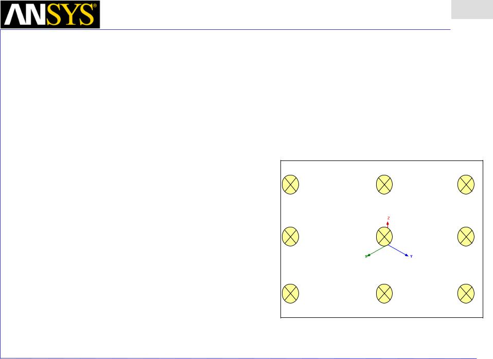
Predefined View Angles
Top
Left |
Right |
Bottom
ANSYS Maxwell Field Simulator v15 – Training Seminar |
P1-23 |
|
|
Maxwell v15 Overview
Presentation
1
•Set Default Material
•To set the default material:
1.Using the 3D Modeler Materials toolbar, choose Select
2.Select Definition Window:
1.Type copper in the Search by Name field
2.Click the OK button
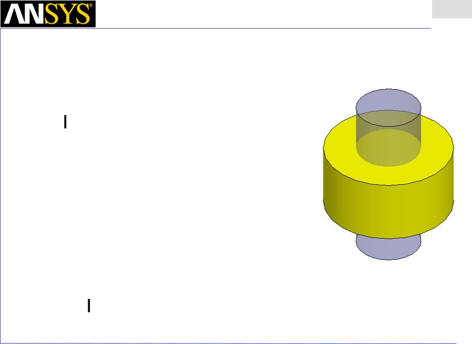
•Create Coil
•To create the coil for the current to flow:
1.Select the menu item Draw > Cylinder
2.Using the coordinate entry fields, enter the center position
•X: 0.0, Y: 0.0, Z: 0.0, Press the Enter key
4.Using the coordinate entry fields, enter the radius of the cylinder
•dX: 0.0, dY: 4.0, dZ: 0.0, Press the Enter key
5.Using the coordinate entry fields, enter the height of the cylinder
•dX: 0.0, dY: 0.0 dZ: 4.0, Press the Enter key
•To set the name:
1.Select the Attribute tab from the Properties window.
2.For the Value of Name type: Coil
3.Click the OK button
•To fit the view:
1.Select the menu item View > Fit All > Active View
|
|
|
|
|
|
|
|
ANSYS Maxwell Field Simulator v15 – Training Seminar |
P1-24 |
||
|
|
|
|
Maxwell v15 Overview
Presentation
1
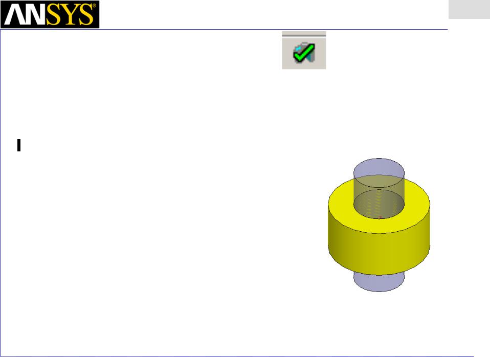
•Overlapping Objects
•About Overlapping Objects
•When the volume of a 3D object occupies the same space as two or more objects you will receive an overlap error during the validation process. This occurs because the solver can not determine which material properties to apply in the area of overlap. To correct this problem, Boolean operations can be used to subtract one object from the other or the overlapping object can be split into smaller pieces that are completely enclosed within the volume of another object. When an object is completely enclosed there will be no overlap errors. In this case, the material of the interior object is used in the area of overlap.
•Complete the Coil
•To select the objects Core and Coil:
1.Select the menu item Edit > Select All
•To complete the Coil:
1.Select the menu item Modeler > Boolean > Subtract
2.Subtract Window
•Blank Parts: Coil
•Tool Parts: Core
•Clone tool objects before subtract: Checked
•Click the OK button
ANSYS Maxwell Field Simulator v15 – Training Seminar |
P1-25 |
|
|
Maxwell v15 Overview
Presentation
1
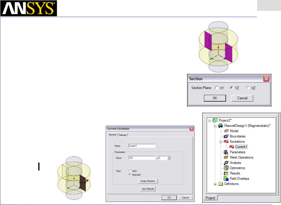
•Create Excitation
•Object Selection
1.Select the menu item Edit > Select > By Name
2.Select Object Dialog,
1.Select the objects named: Coil
2.Click the OK button
•Section Object
1.Select the menu item Modeler > Surface > Section
1.Section Plane: YZ
2.Click the OK button
•Separate Bodies
1.Select the menu item Modeler > Boolean > Separate Bodies
2.Delete the extra sheet which is not needed
•Assign Excitation
1.Select the menu item Maxwell 3D> Excitations > Assign > Current
2.Current Excitation : General
1.Name: Current1
2.Value: 120 A
3.Type: Stranded
3.Click the OK button
ANSYS Maxwell Field Simulator v15 – Training Seminar |
P1-26 |
|
|
Maxwell v15 Overview
Presentation
1
•Show Conduction Path
•Show Conduction Path
1.Select the menu item Maxwell 3D> Excitations > Conduction Path > Show Conduction Path
2.From the Conduction Path Visualization dialog, select the row1 to visualize the conduction path in on the 3D Model.
3.Click the Close button
•Fix Conduction Path
•To solve this isolation problem an insulating boundary condition will be used.
1.Select the outer face of the core by typing f on the keyboard and select the outer face of the core.
2.Select the menu item Maxwell 3D> Boundaries > Assign > Insulating
3.Insulating Boundary
1.Name: Insulating1
2.Click the OK button
4.Follow the instructions from above to redisplay the Conduction Path
ANSYS Maxwell Field Simulator v15 – Training Seminar |
P1-27 |
|
|
Maxwell v15 Overview
Presentation
1
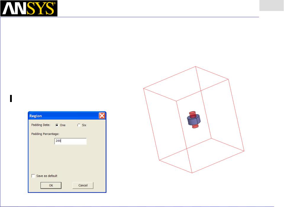
•Define a Region
•Before solving a project a region has to be defined. A region is basically an outermost object that contains all other
objects. The region can be defined by a special object in Draw > Region. This special region object will be resized automatically if your model changes size.
•A ratio in percents has to be entered that specifies how much distance should be left from the model.
•To define a Region:
1.Select the menu item Draw > Region
1.Padding Data: One
2.Padding Percentage: 200
3.Click the OK button
Note: Since there will be considerable fringing in this device, a padding percentage of at least 2 times, or 200% is recommended
ANSYS Maxwell Field Simulator v15 – Training Seminar |
P1-28 |
|
|
Maxwell v15 Overview
Presentation
1
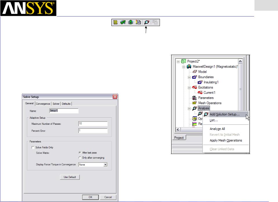
•Maxwell - Solution Setup
•Creating an Analysis Setup
Add Solution Setup
•To create an analysis setup:
1.Select the menu item Maxwell 3D> Analysis Setup > Add Solution Setup
2.Solution Setup Window:
1.Click the General tab:
•Maximum Number of Passes: 10
•Percent Error: 1
2.Click the OK button
ANSYS Maxwell Field Simulator v15 – Training Seminar |
P1-29 |
|
|
Maxwell v15 Overview
Presentation
1
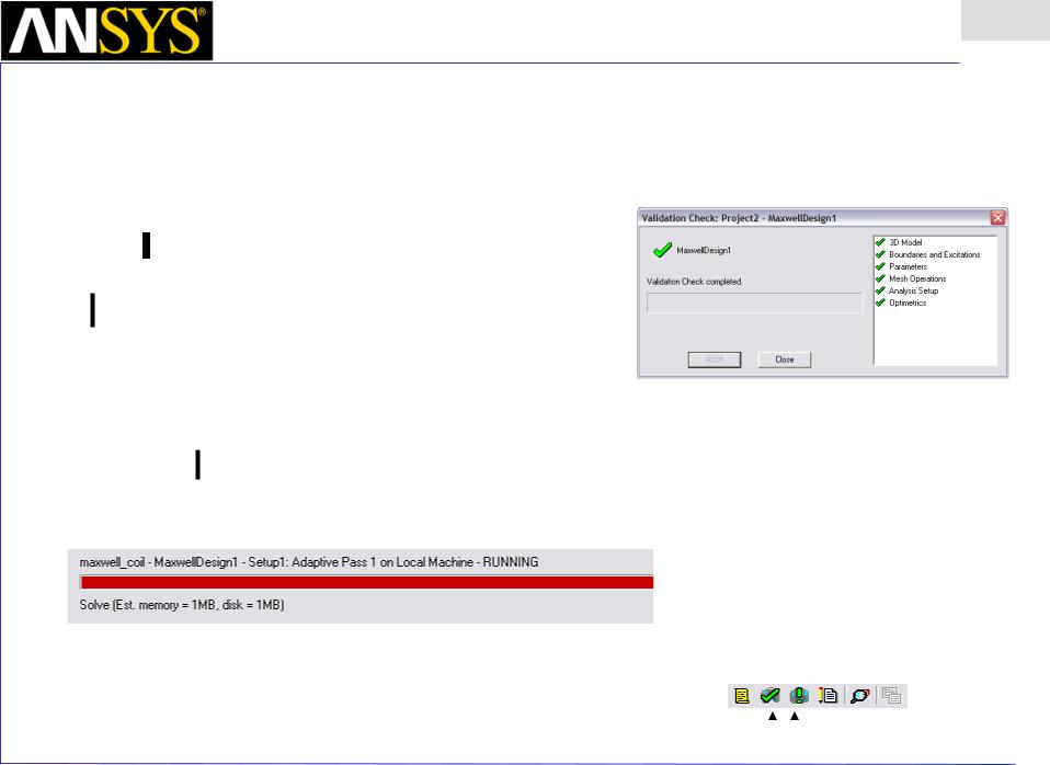
•Save Project
•To save the project:
1.In an Maxwell window, select the menu item File > Save As.
2.From the Save As window, type the Filename: maxwell_coil
3.Click the Save button
•Analyze
•Model Validation
•To validate the model:
1.Select the menu item Maxwell 3D> Validation Check
2.Click the Close button
•Note: To view any errors or warning messages, use the Message Manager.
•Analyze
•To start the solution process:
1.Select the menu item Maxwell 3D> Analyze All
|
|
|
|
|
|
|
|
|
|
|
|
|
|
|
|
|
|
|
|
|
|
|
|
|
|
|
|
|
|
|
|
|
|
|
|
|
|
|
|
|
|
|
|
|
|
|
|
|
|
|
|
|
|
|
|
|
|
|
|
|
|
|
|
Validate |
|
|
|
Analyze All |
|||
|
|
|
|
|
|
|
|||||
|
|
|
|
|
|||||||
|
|
|
|
|
|
|
|
|
|
|
|
ANSYS Maxwell Field Simulator v15 – Training Seminar |
|
|
|
|
P1-30 |
||||||
|
|
|
|
|
|
|
|
|
|
|
|
Maxwell v15 Overview
Presentation
1
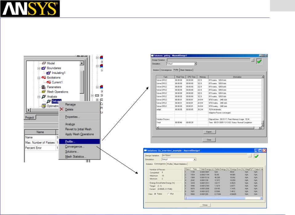
•View detailed information about the progress
•In the Project Tree click on Analysis->Setup1 with the right mouse button und select Profile
|
|
|
|
|
|
|
|
ANSYS Maxwell Field Simulator v15 – Training Seminar |
P1-31 |
||
|
|
|
|
Maxwell v15 Overview
Presentation
1
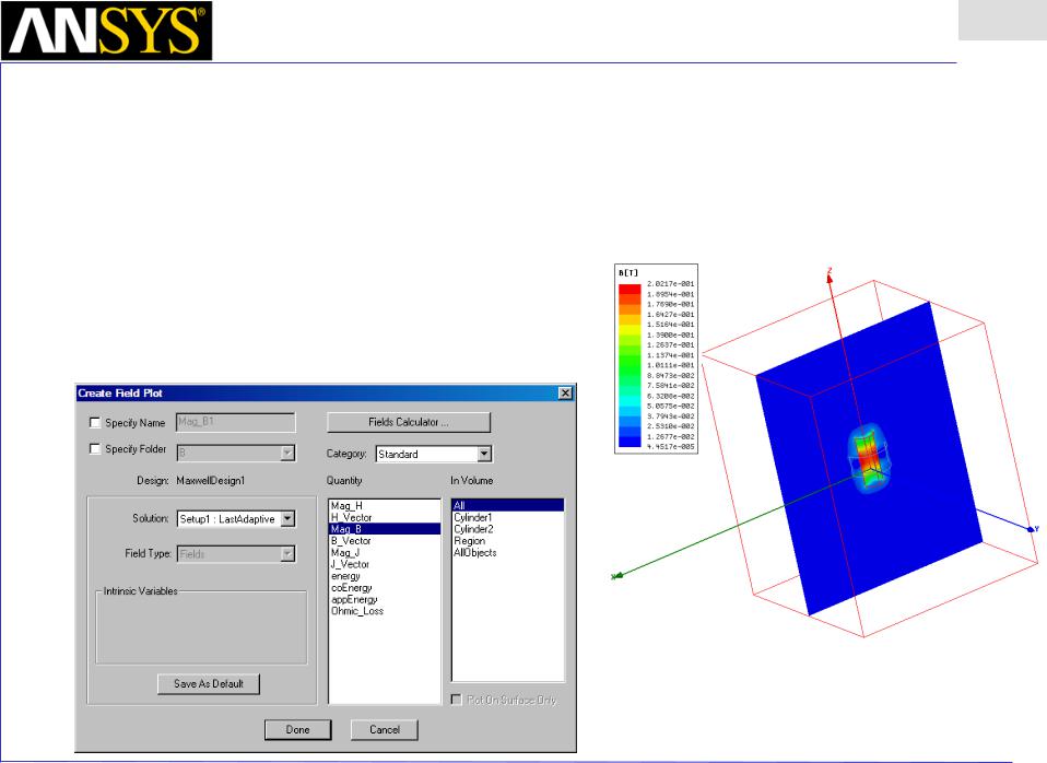
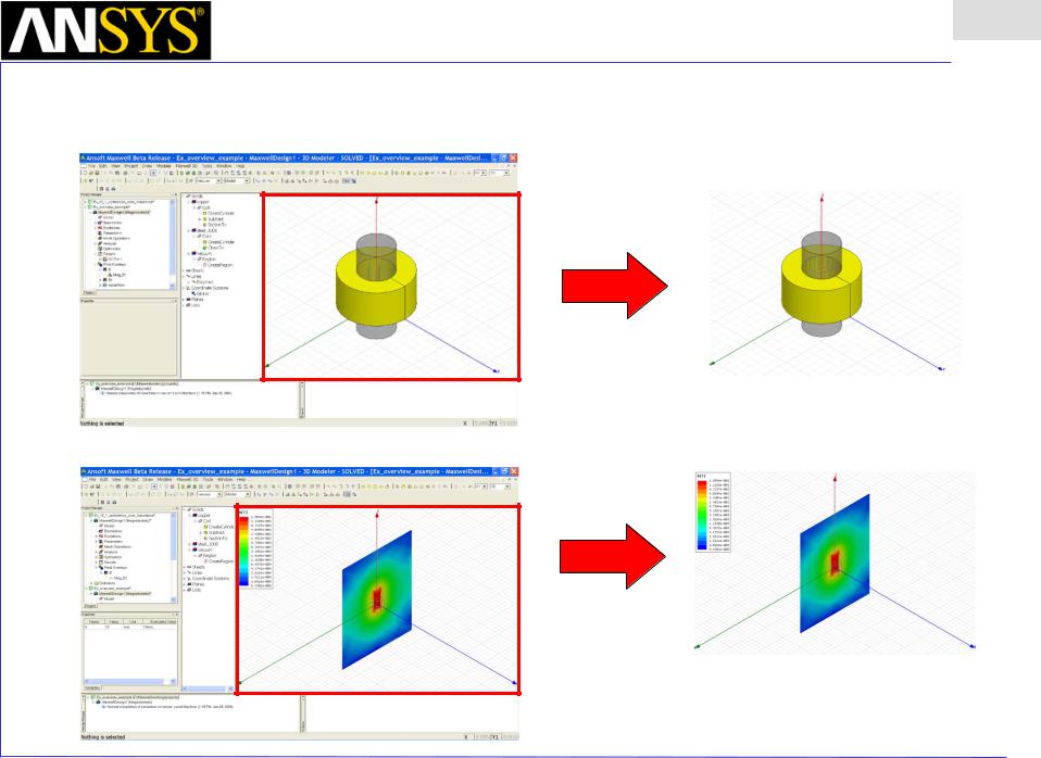
•Field Overlays
•To create a field plot:
1.Select the Global XZ Plane
1.Using the Model Tree, expand Planes
2.Select Global:XZ
2.Select the menu item Maxwell > Fields > Fields > B > Mag_B
3.Create Field Plot Window
1.Solution: Setup1 : LastAdaptive
2.Quantity: Mag_B
3.In Volume: All
4.Click the Done button
ANSYS Maxwell Field Simulator v15 – Training Seminar |
P1-32 |
|
|
Maxwell v15 Overview
Presentation
1
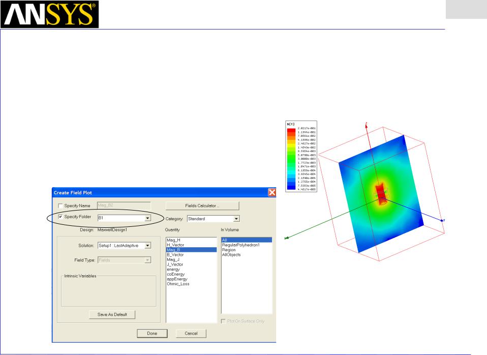
•Field Overlays
•To create a second field plot of same quantity, but different scale:
1.Select the Global XZ Plane
1.Using the Model Tree, expand Planes
2.Select Global:XZ
2.Select the menu item Maxwell 3D> Fields > Fields > B > Mag_B
3.Create Field Plot Window
1.Specify Folder: B1
2.Solution: Setup1 : LastAdaptive
3.Quantity: Mag_B
4.In Volume: All
5.Click the Done button
ANSYS Maxwell Field Simulator v15 – Training Seminar |
P1-33 |
|
|
Maxwell v15 Overview
Presentation
1
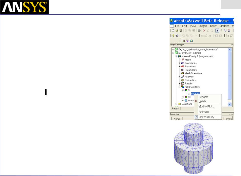
•To modify a Magnitude field plot:
1.Select the menu item Maxwell 3D> Fields > Modify Plot Attributes
2.Select Plot Folder Window:
1.Select: B
2.Click the OK button
3.B-Field Window:
1.Click the Scale tab
1.Scale: Log
2.Click the Close button
4.Hide the plots by clicking in the project tree and unchecking Plot Visibility
•Mesh Overlay
•To select the objects Core and Coil:
1.Select the menu item Edit > Select > By Name
2.Press and hold the CTRL key and select Core and Coil from the list
3.Click the OK button
•To create a mesh plot:
1.Select the menu item Maxwell 3D> Fields > Plot Mesh
2.Create Mesh Window:
1.Click the Done button
ANSYS Maxwell Field Simulator v15 – Training Seminar |
P1-34 |
|
|
Maxwell v15 Overview
Presentation
1
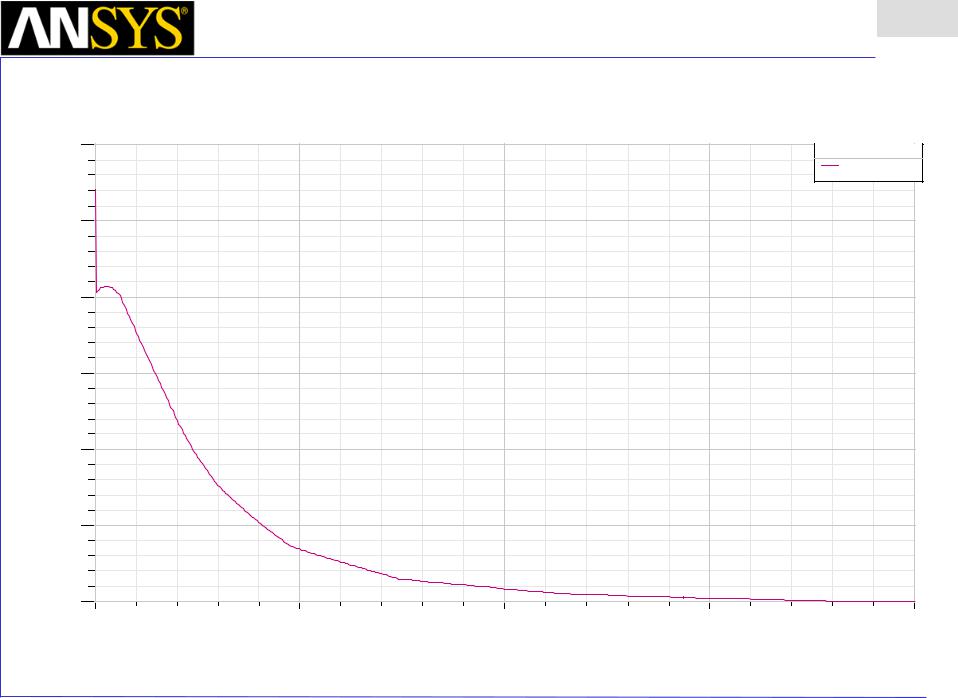
•Plot the z-component of B Field along the line
1.Create a line
2.Calculate the z-component of B using the Calculator tool
3.Create report – plot the desired graph
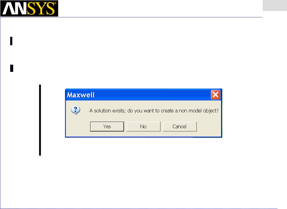
• To create a line
1. Select the menu item Draw > Line. The following window opens:
2.Answer YES to create a non model object and not to destroy the solution.
3.Place the cursor at the top face of the core and let the cursor snap to the center.
4.Click the left mouse button and hold the z button on the keyboard while moving the cursor up. Left click at some distance from the core and double click left to end the line.
5.Leave the values in the upcoming dialog box and close the dialog by pressing OK.
|
|
|
|
|
|
|
|
ANSYS Maxwell Field Simulator v15 – Training Seminar |
P1-35 |
||
|
|
|
|
Maxwell v15 Overview
Presentation
1
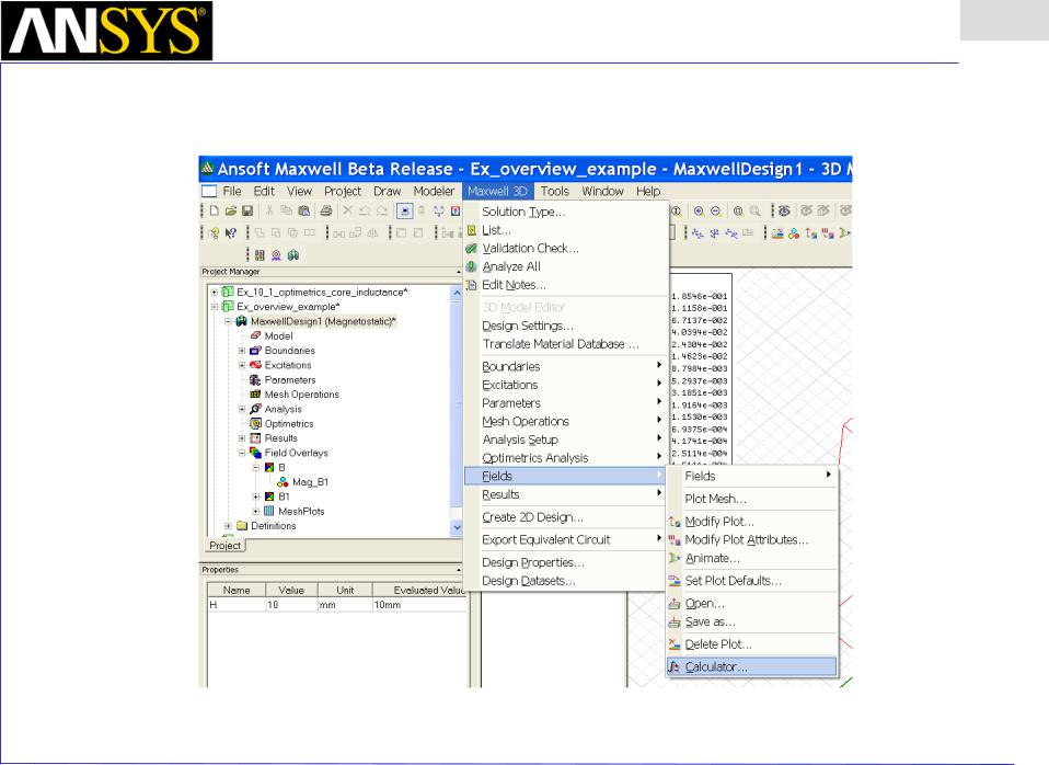
•To bring up the Calculator tool
1.Select the menu item Maxwell 3D> Fields- > Calculator
|
|
|
|
|
|
|
|
ANSYS Maxwell Field Simulator v15 – Training Seminar |
P1-36 |
||
|
|
|
|
 Maxwell v15
•To calculate the z-component of B field
1.In the Input Column select the Quantity B
2.In the Vector Column select the ScalarZ component
3.In the General Column select Smooth
4.Press the Add button in the upper
part of the calculator and enter a name that describes the calculation
-enter Bz for B field in z-direction
5.Click Done to close the calculator
Presentation
Overview 1
ANSYS Maxwell Field Simulator v15 – Training Seminar |
P1-37 |
|
|
Maxwell v15 |
Overview |
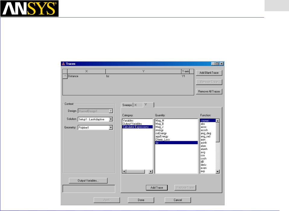
•To create report (plot the desired graph)
1.Select the menu item Maxwell 3D> Result > Create Report
2.Enter Fields and Rectangular Plot and click the OK button
3.Select the following: Geometry – Polyline1; Category – Calculator Expressions; Quantity – Bz
4.Press the Add Trace to copy your selection to the upper part of the window and click on the Done button
Presentation
1
|
|
|
|
|
|
|
|
ANSYS Maxwell Field Simulator v15 – Training Seminar |
P1-38 |
||
|
|
|
|
|
|
Maxwell v15 |
|
|
|
Presentation |
|
|
|
|
Overview |
1 |
|
|
|
|
|
|
||
Ansoft Corporation |
|
XY Plot 1 |
|
|
MaxwellDesign1 |
|
0.030 |
|
|
|
|
Curve Info |
|
|
|
|
|
|
||
|
|
|
|
|
Bz |
|
|
|
|
|
|
Setup1 : LastAdaptive |
|
0.025 |
|
|
|
|
|
|
0.020 |
|
|
|
|
|
|
Bz0.015 |
|
|
|
|
|
|
0.010 |
|
|
|
|
|
|
0.005 |
|
|
|
|
|
|
0.000 |
0.00 |
5.00 |
10.00 |
15.00 |
|
20.00 |
|
|
|
Distance [mm] |
|
|
|
ANSYS Maxwell Field Simulator v15 – Training Seminar |
P1-39 |
|
|
Maxwell v15 Overview
Presentation
1
•To save drawing Window or a plot to clipboard
1.Select the menu item Edit > Copy Image
ANSYS Maxwell Field Simulator v15 – Training Seminar |
P1-40 |
|
|
 Maxwell v15
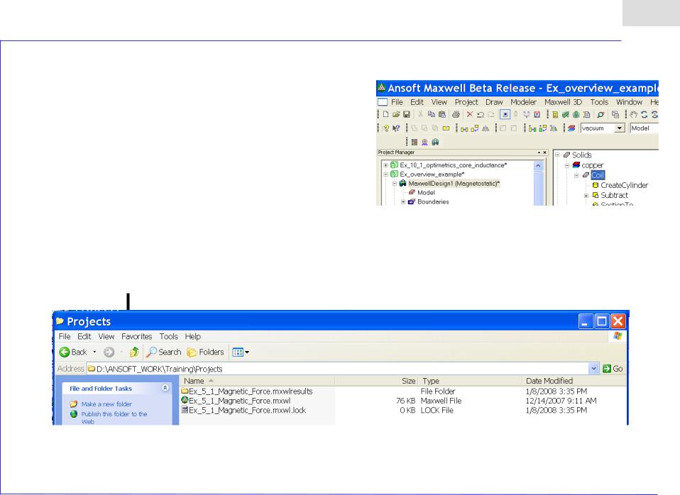
•File Structure
•Everything regarding the project is stored in an ascii file
•File: <project_name>.mxwl
•Double click from Windows Explorer will open and launch Maxwell 3D
•Results and Mesh are stored in a folder named <project_name>.mxwlresults
•Lock file: <project_name>.lock.mxwl
•Created when a project is opened
•Auto Save File: <project_name>.mxwl.auto
•When recovering, software only checks date
Presentation
Overview 1
•
•
If an error occurred when saving the auto file, the date will be newer then the original
Look at file size (provided in recover dialog)
ANSYS Maxwell Field Simulator v15 – Training Seminar |
P1-41 |
|
|
Maxwell v15 Overview
Presentation
1
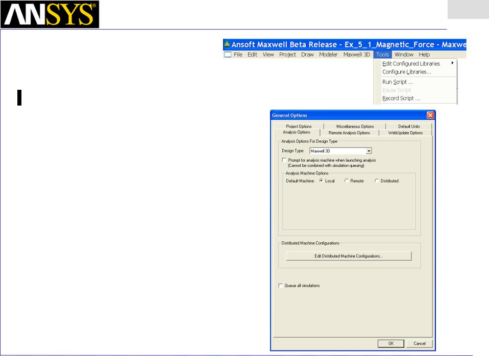
•Scripts
•Default Script recorded in Maxwell
•Visual Basic Script
•Remote Solve (Windows Only)
•Tools > Options > General Options > Analysis Options
ANSYS Maxwell Field Simulator v15 – Training Seminar |
P1-42 |
|
|
Maxwell v15 Overview
Presentation
1
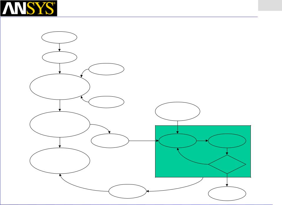
•The Process
Design
Solution Type
2. Boundaries
1. Parametric Model
Geometry/Materials
2. Excitations
3. Mesh
Operations
2. Analysis Setup
Solution Setup
Frequency Sweep
Analyze |
Mesh |
Solve |
|
Refinement |
|||
|
|
4. Results |
|
|
|
2D Reports |
|
NO |
Converged |
Fields |
|
|
|
|
2. Solve Loop |
|
|
|
|
|
|
|
|
|
YES |
|
Update |
|
Finished |
|
|
|
ANSYS Maxwell Field Simulator v15 – Training Seminar |
P1-43 |
|
|
|
Maxwell v15 |
Overview |
Presentation |
|
|
|
|
||
|
|
|
1 |
|
|
|
|
|
|
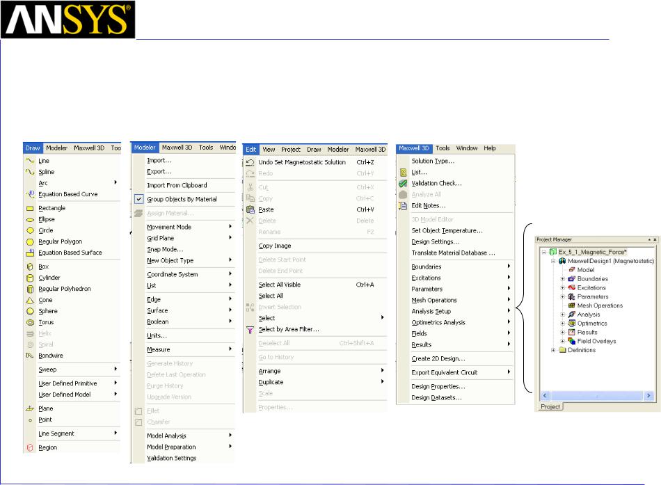
• |
Menu Structure |
Note: |
|
|
• Edit Copy/Paste is a dumb copy for only dimensions and |
|
|||
|
• Draw – Primitives |
|
||
|
materials, but not the history |
|
|
|
|
• Modeler – Settings and Boolean Operations |
• Edit > Duplicate clones objects include dimensions, |
|
|
|
• Edit – Copy/Paste, Arrange, Duplicate |
materials and the creation history with all variables |
|
|
|
|
|
|
|
|
|
|
|
|
•Maxwell 3D– Boundaries, Excitations, Mesh Operations, Analysis Setup, Results
ANSYS Maxwell Field Simulator v15 – Training Seminar |
P1-44 |
|
|
Maxwell v15 Overview
Presentation
1
•Modeler – Model Tree
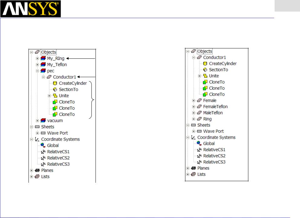
•Select menu item Modeler > Group by Material
Material
Object
Object Command History
Grouped by Material |
Object View |
ANSYS Maxwell Field Simulator v15 – Training Seminar |
P1-45 |
|
|
Maxwell v15 Overview
Presentation
1
•Modeler – Commands
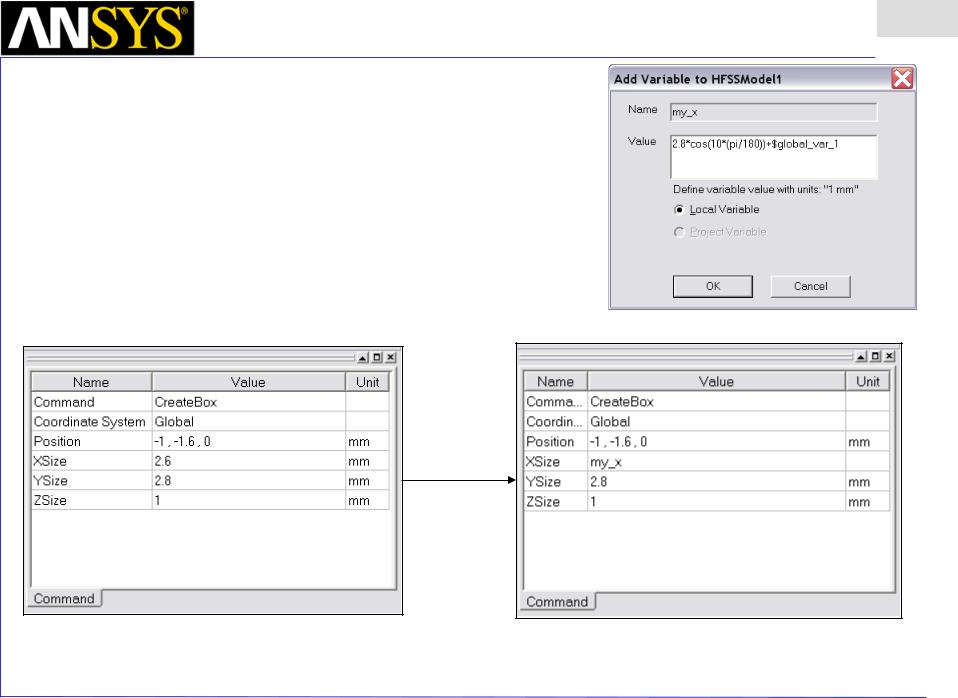
•Parametric Technology
•Dynamic Edits - Change Dimensions
•Add Variables
•Project Variables (Global) or Design Variables (Local)
•Animate Geometry
•Include Units – Default Unit is meters
•Supports mixed Units
ANSYS Maxwell Field Simulator v15 – Training Seminar |
P1-46 |
|
|
 Maxwell v15
•Modeler – Primitives
•2D Draw Objects
•The following 2D Draw objects are available:
•Line, Spline, Arc, Equation Based Curve,
Rectangle, Ellipse, Circle, Regular Polygon,
Equation Based Surface
•3D Draw Objects
•The following 3D Draw objects are available:
•Box, Cylinder, Regular Polyhedron
Cone, Sphere, Torus, Helix, Spiral, Bond Wire
•True Surfaces
•Circles, Cylinders, Spheres, etc are represented as true surfaces. In versions prior to release 11 these primitives would be represented as faceted objects. If you wish to use the faceted primitives, select the Regular Polyhedron or Regular Polygon.
Toolbar: 2D Objects |
Toolbar: 3D Objects |
Presentation
Overview 1
ANSYS Maxwell Field Simulator v15 – Training Seminar |
P1-47 |
|
|