

2 lec Eng
.pdfDirect method of Stability analysis
u(t)
Input signal
System
y(t)
Output signal
W s |
|
|
y(s) |
|
|
b sm b sm 1 |
... b |
|
|
s b |
|||||||||
|
|
|
|
0 |
|
1 |
|
|
|
m 1 |
|
m |
|
||||||
|
|
|
|
|
sn a sn 1 |
|
|
|
|
|
|
|
|||||||
|
|
|
u(s) |
|
|
a |
... a |
n 1 |
s a |
n |
|||||||||
|
|
|
|
|
|
0 |
|
1 |
|
|
|
|
|
|
|
||||
The equation |
|
a |
sn a sn 1 |
... a |
n 1 |
s a |
n |
0 |
is called |
||||||||||
|
|
0 |
|
|
1 |
|
|
|
|
|
|
|
|
|
|||||
characteristic equation.
The roots of this equation 1 , 2 , ... , n are called poles of the system (or the transfer function)
Direct method of Stability analysis
Let |
W s |
s 1 |
1 |
1; |
|
||
|
|
The poles: |
|
|
|
||
s 1 2s 1 |
|
1 |
|
||||
|
|
2 |
|
. |
|||
|
|
|
|
2 |
|||
|
|
|
|
|
|
|
|
The impulse response for this system is
y t 2e 1 t 32 e 12 t
The exponential terms e i t control the response y t as t
The real parts of the poles must be negative
Direct method of Stability analysis
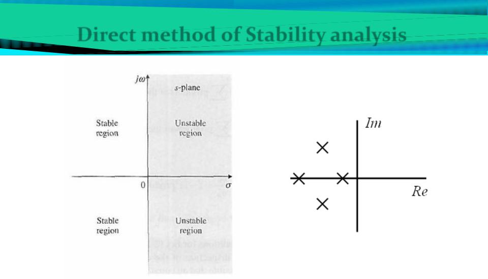
For asymptotic stability the roots of the characteristic equation must all be located in the left-half s-plane.
Direct method of Stability analysis
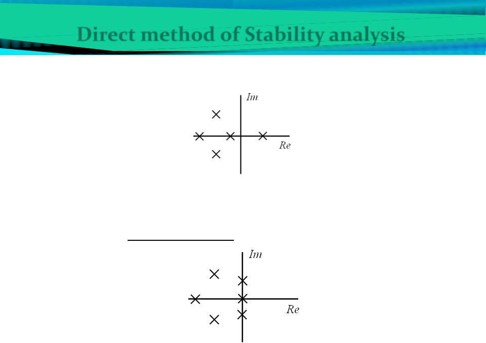
If there is at least one pole located in the right-half s-plane, the system is unstable:
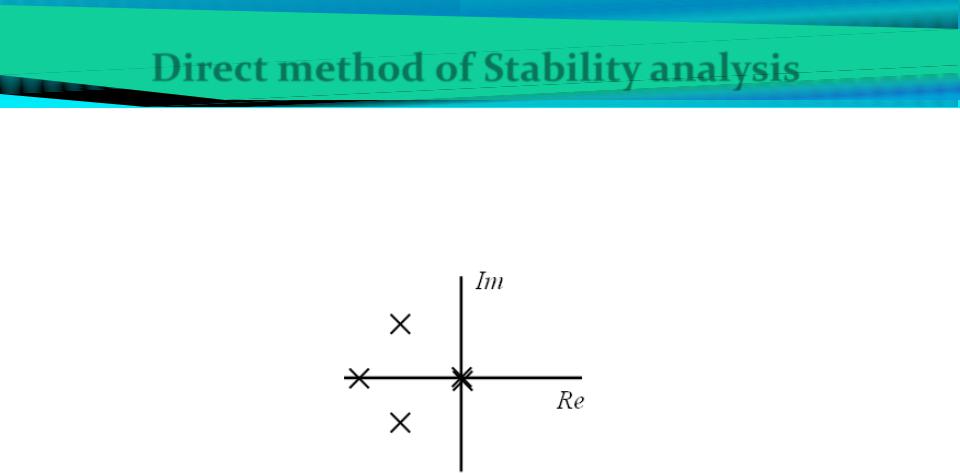
If there is no one pole located in the right-half s-plane, but there are one or more poles directly on the imaginary axis, the system is neutral stable:
Direct method of Stability analysis
There is an exception.
In the case of multiple poles in the imaginary axis, the system is unstable:
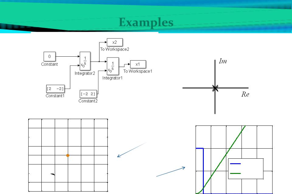
Examples
1. |
W s |
1 |
|
||
|
s2 |
|
|
|
s-plane
x2
4 
3
2 


1
0 |
Equilibrium |
|
|
-1 |
position |
-2 


-3
-4 |
|
|
|
|
|
|
-15 |
-10 |
-5 |
0 |
5 |
10 |
15 |
x1
1.5
zero-input
1 |
|
|
|
|
|
|
|
|
input |
|
|
0.5 |
|
|
output |
|
|
|
|
|
|
||
zero-state |
|
|
|
|
|
00 |
1 |
2 |
3 |
4 |
5 |
|
|
time, sec |
|
|
|
|
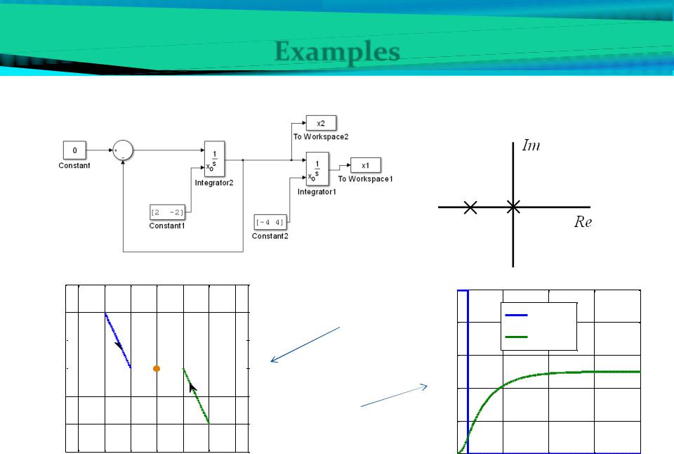
Examples |
||
2. |
1 |
|
|
|
W s |
|
|
|
s s 1 |
||
s-plane
x2
3 
2
1 


0 


|
|
|
Equilibrium |
|
|
|
-1 |
|
|
position |
|
|
|
|
|
|
|
|
|
|
-2 |
|
|
|
|
|
|
-3 |
|
|
|
|
|
|
-6 |
-4 |
-2 |
0 |
2 |
4 |
6 |
x1
zero-input
zero-state
1 |
|
|
|
|
0.8 |
|
input |
|
|
|
|
|
|
|
|
|
output |
|
|
0.6 |
|
|
|
|
0.4 |
|
|
|
|
0.2 |
|
|
|
|
00 |
2 |
4 |
6 |
8 |
|
|
time, sec |
|
|
|
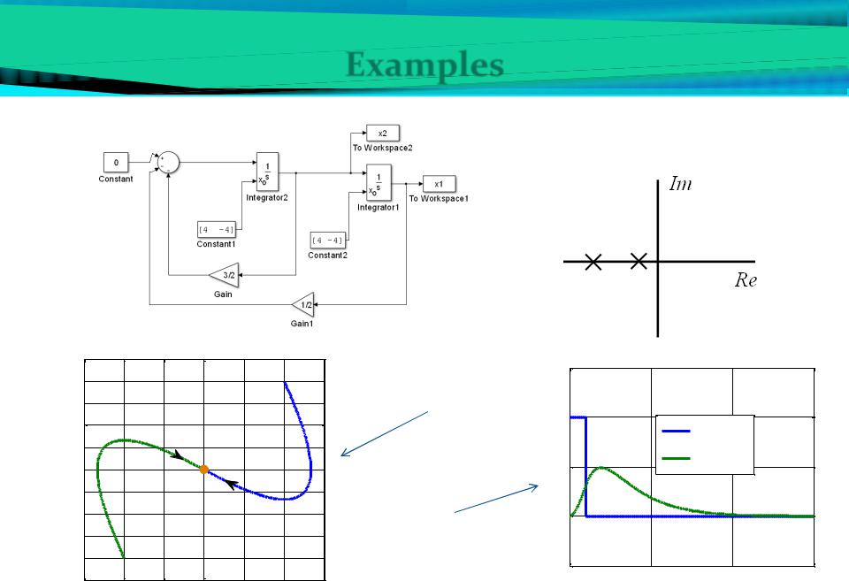
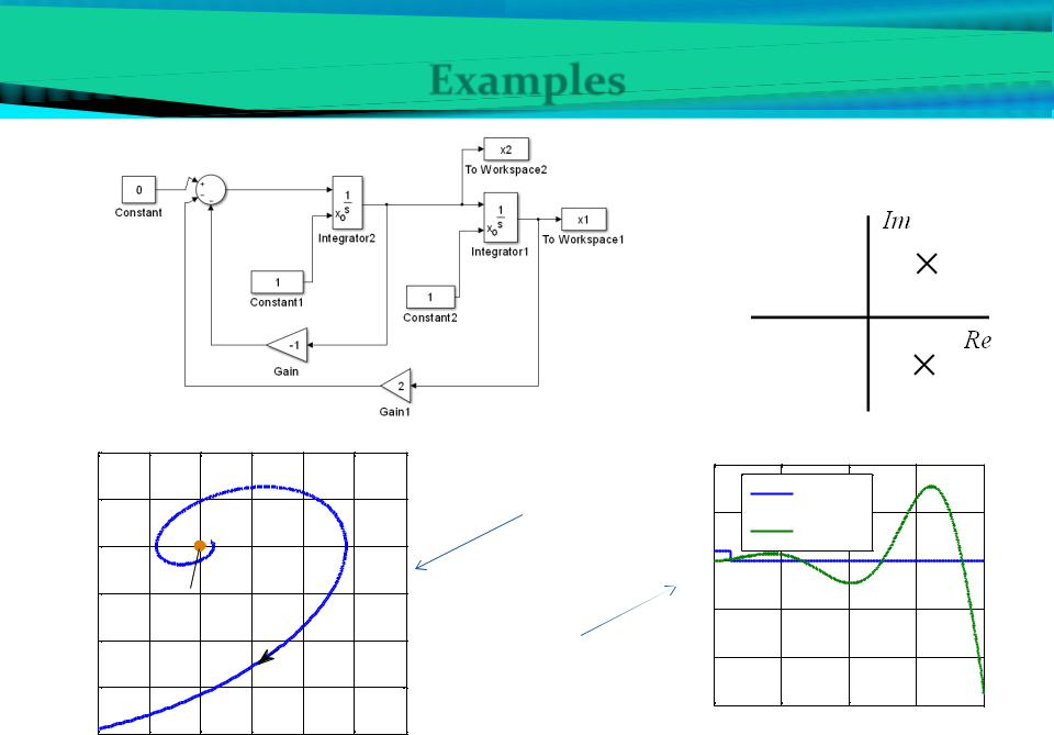
Examples |
||
3. |
1 |
|
|
|
W s |
|
|
|
s 1 2s 1 |
||
s-plane
|
5 |
|
|
|
|
|
|
|
4 |
|
|
|
|
|
|
|
3 |
|
|
|
|
|
|
|
2 |
|
|
|
|
|
|
|
1 |
|
|
|
|
|
|
x2 |
0 |
|
|
|
|
|
|
|
|
|
|
|
|
|
|
|
-1 |
|
|
|
|
|
|
|
-2 |
|
Equilibrium |
|
|
|
|
|
|
position |
|
|
|
||
|
|
|
|
|
|
||
|
-3 |
|
|
|
|
|
|
|
-4 |
|
|
|
|
|
|
|
-5 |
|
|
|
|
|
|
|
-6 |
-4 |
-2 |
0 |
2 |
4 |
6 |
|
|
|
|
x1 |
|
|
|
zero-input
zero-state
1.5 |
|
|
|
1 |
|
input |
|
|
|
|
|
0.5 |
|
output |
|
|
|
|
|
0 |
|
|
|
-0.50 |
5 |
10 |
15 |
|
|
time, sec |
|
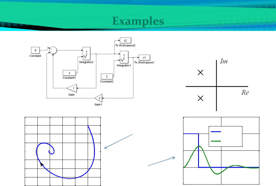
Examples
4. |
|
|
|
|
1 |
|
||
|
|
|
|
|
|
|
||
W s |
1 |
s2 |
|
1 |
s 1 |
|||
|
||||||||
|
|
|
||||||
|
2 |
|
|
2 |
|
|||
s-plane
x2
4 
3
2
1
0 


-1 |
|
Equilibrium |
|
|
|
|
|
|
|
|
|
||
-2 |
|
position |
|
|
|
|
-3 |
|
|
|
|
|
|
-4 |
|
|
|
|
|
|
-2 |
-1 |
0 |
1 |
2 |
3 |
4 |
x1
zero-input
zero-state
1.5 |
|
|
1 |
input |
|
|
|
|
|
output |
|
0.5 |
|
|
0 |
|
|
-0.50 |
5 |
10 |
|
time, sec |
|
Examples |
W s |
|
|
|
1 |
|
|
|
|
|
|
|
|||
5. |
|
1 2 |
1 |
|
|||
|
|
|
s |
|
|
s 1 |
|
|
|
|
2 |
2 |
|||
s-plane
|
20 |
|
|
|
|
|
|
|
10 |
|
|
|
|
|
|
|
0 |
|
|
|
|
|
|
x2 |
-10 |
|
Equilibrium |
|
|
|
|
|
|
|
|
|
|||
|
|
|
|
|
|
||
|
|
|
position |
|
|
|
|
|
-20 |
|
|
|
|
|
|
|
-30 |
|
|
|
|
|
|
|
-40 |
|
|
|
|
|
|
|
-10 |
-5 |
0 |
5 |
10 |
15 |
20 |
|
|
|
|
x1 |
|
|
|
zero-input
zero-state
10
5 |
|
input |
|
|
|
|
|
|
|
|
|
output |
|
|
0 |
|
|
|
|
-5 |
|
|
|
|
-10 |
|
|
|
|
-150 |
2 |
4 |
6 |
8 |
|
|
time, sec |
|
|