Damped oscillator

_{Solve the damped oscillator problem}

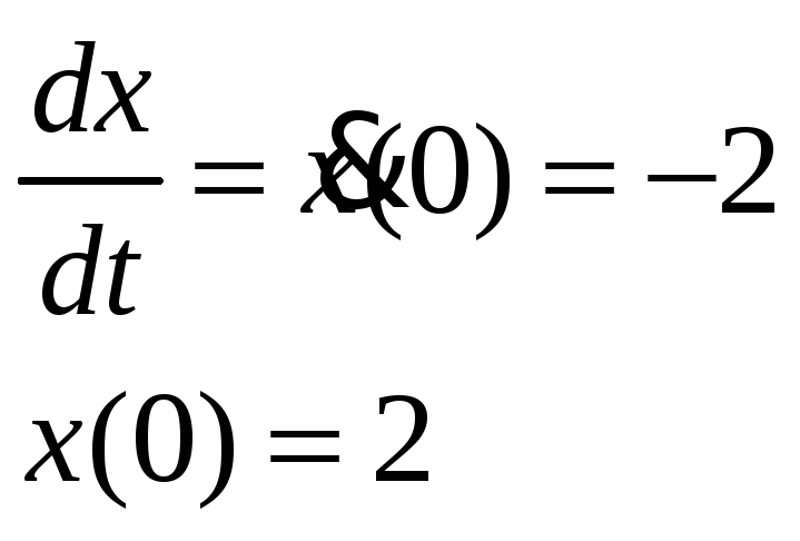
_{Assume that u(t) = 0, that is, there is no input.}

_{PURPOSE: To illustrate how to configure a SIMULINK diagram for a higher order differential equation and how to introduce initial conditions into it.}

_{SOLUTION: Solve equation first with respect to the highest order derivative to obtain}

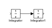
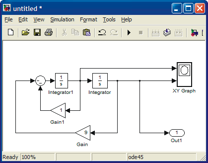
_{To set up the right-hand side two integrators are needed:}

_{The input to the first integraror is the second derivative and its output is . The latter is the innput to the second integrator producing x(t) at its output. In this way we have constructed the left-hand side of the equation. Since the second derivative is equal to the right hand side, we collect it term by term. In order to do that we need from the output of the first integrator, x(t) from the output of the second integrator and u(t), the step input must be generated. Here x(t) must also be multiplied by 9, so a gain is required. All these items are to be summed up so a sum block is also needed. The final configuration is given below. The initial values are added to the integrators. The resulting configuration is given below.}

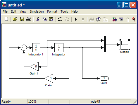
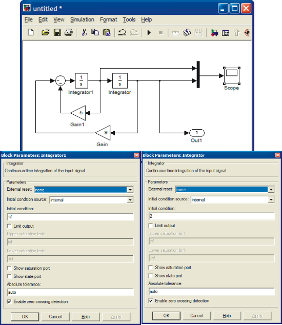
_{Next, set up the initial conditions by clicking the integrators one at a time and making appropriate changes.}

_{The solution x(t) and are shown in Fig. below. The first figure is SIMULINK scope and the second is the result from Command window simulation.}

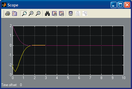
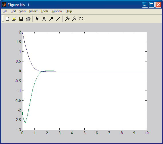
_{The sharpness of the lower curve around t = 0.4 s is not real, it should be smooth. First you might suspect numerical difficulties (there are none) due to too large a step size. This is not the case. It is due to display graphics, i.e., not enough points have been saved to have a smooth presentation.}

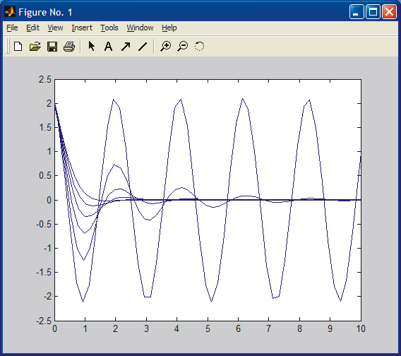
_{The damping factor can be changed by changing the coefficient 5 in front of . If the coefficient is zero (no damping), the result is a sinusoidal. Increasing the damping will result in damping oscillations. Complete the study to obtain the following responses.}

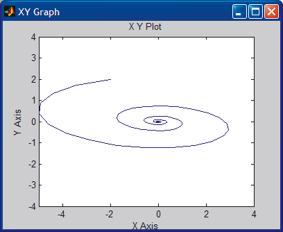
Let us also plot a phase plane plot (x vs dx/dt). Note that here time has been eliminated. To see the effect better, start with less damping. Change the coefficient 5 to 1.

The result is shown below.

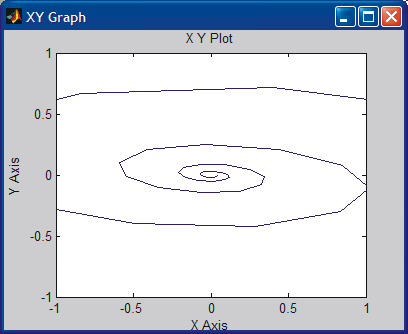
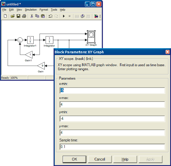
Xy Graph does not adjust the scales automatically. In order to see the whole picture, click the xy Graph open and adjust the scales. Adjusting also the Sample time results in smooth picture.

CONCLUSION: A stable system. It converges towards the origin. Physical interpretation: In origin both position and velocity are zero.