

grigorenko2001
.pdfPHYSICAL REVIEW C, VOLUME 64, 054002
Two-proton radioactivity and three-body decay: General problems and theoretical approach
L. V. Grigorenko,1,2 R. C. Johnson,1 I. G. Mukha,3,2 I. J. Thompson,1 and M. V. Zhukov4
1Department of Physics, University of Surrey, Guildford GU2 7XH, United Kingdom 2Russian Research Center ``The Kurchatov Institute,'' RU-123182 Moscow, Russia 3GSI, Planckstrasse 1, D-64291 Darmstadt, Germany
4Department of Physics, Chalmers University of Technology, S-41296 GoÈteborg, Sweden
and GoÈteborg University, S-41296 GoÈteborg, Sweden
~Received 27 April 2001; published 4 October 2001!
Theoretical aspects of the two-proton radioactivity and three-body decays are studied for nuclear systems, where three-body channel is the only ~or dominating! decay channel. We brie¯y review the current experimental and theoretical status of the problem. We discuss the applicability of the widely used qualitative models ~e.g., diproton model, direct decay to continuum! for estimates of the two-proton radioactivity. A three-body model is developed, which is free of most uncertainties typical for these estimates. It employs various forms of approximate boundary conditions for the three-body Coulomb problem and demonstrates high stability for widths and spatial distributions.
DOI: 10.1103/PhysRevC.64.054002 |
PACS number~s!: 21.60.Gx, 21.45.1v, 23.50.1z, 21.10.Tg |
I. INTRODUCTION
Nuclear decays with three ~and more! fragments in the ®nal state are very exotic processes. They have been investigated experimentally in many nuclei, with the hope that the highly exclusive information obtained in such studies will make them valuable. Two-proton radioactivity belongs to these exotic processes and it represents an essential part of experimental and theoretical studies of the proton-rich nuclei either in the vicinity or beyond the proton dripline @1#.
Some qualitative theoretical results for these exotic processes have been obtained in the early papers @2± 6#, and an overview of the results up to 1972 can be found in @7#. Since that time little progress has been achieved in the theory of such processes, and two-proton emission and b-delayed multiparticle emission have never been thoroughly studied using the few-body methods possible with modern techniques. Here we mention the papers @8 ±11# employing three-body amplitudes for phenomenological analysis of the experimental data, and continuum calculations of Ref. @12# for A56 nuclei. In a recent paper @13# we used for the ®rst time a three-body model to calculate the two-proton decay process. In this work we expand the effort of Ref. @13#, and provide a more complete discussion of the method.
We discuss ®rst the general problems of two-proton radioactivity and three-body decay studies. We brie¯y review the notation of hyperspherical harmonic ~HH! method used in this paper, and the different coordinate systems convenient for discussion of three-body decays. In Sec. II we discuss various estimates that are possible in the context of the threebody decay problem, and try to demonstrate the failure of attempts to ®nd an adequate quasiclassical description, and hence that a more complete few-body theory is required. In Sec. III we describe the three-body models that can be applied to the phenomenon.
A. General problems
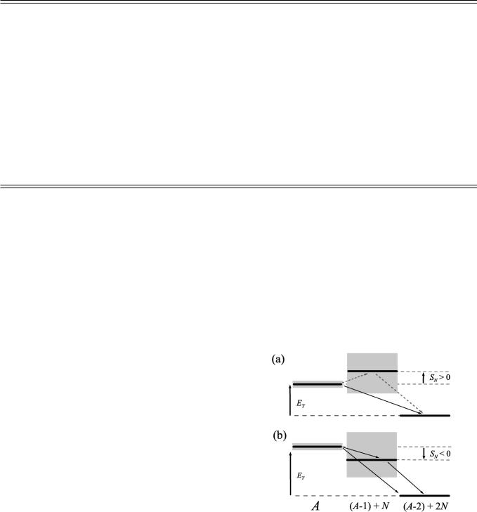
We can distinguish two different modes of three-body decay. The ®rst mode is referred to as ``true three-body decay''
in the pioneering work of Goldansky @2#, where the concept of two-proton radioactivity was suggested. In this mode the three-body decay occurs because the one-proton breakup threshold is higher than two-proton breakup threshold @Fig. 1~a!#. In other words, the ground state resonances in the core1p subsystem are located higher than in the composite core1p1p system. Ironically this decay mode is still unidenti®ed in the medium mass proton-rich nuclei, where it was initially predicted @2#. However, the three-body decay mode has been well studied in the light ~including neutron-
rich! clusterized systems. The following states decay as core1N1N: @8,9#, @8#, 6Be 01 and 21
@8,6#, 8He 21 ~@14# and references therein!, 10He 01 @15±
FIG. 1. Energy conditions for different modes of the twonucleon emission ~three-body decay!: true three-body decay ~a!, sequential decay ~b!, and situation with binary channel open ~c!.
0556-2813/2001/64~5!/054002~12!/$20.00 |
64 054002-1 |
©2001 The American Physical Society |
GRIGORENKO, JOHNSON, MUKHA, THOMPSON, AND ZHUKOV |
PHYSICAL REVIEW C 64 054002 |
TABLE I. Nuclear states with dominant three-body decay nuclear channel. In the upper part of the table those states that satisfy the condition of true three-body decay are shown; the lower part gives the states with possible binary decay channels. E* is the excitation energy relative to the ground state ~if applicable!, ET is the energy above the three-body breakup threshold. The last column gives the information about the lowest states in the subsystems in the format `` AZ: Jp, ER , G; '' with two-body resonance characteristics ER and G given in keV. Columns ``Exp.'' and ``Th.'' give the references for relevant experimental and theoretical papers.
ZAZ |
Jp |
E*, keV |
ET , keV |
G, keV |
Channel |
Jcpore |
Exp. |
Th. |
Lowest states in subsystems |
26He |
21 |
1797~25! |
825 |
113~20! |
a1n1n |
01 |
@21# |
@8# |
5He: 3/22, 890, 600 |
46Be |
01 |
g.s. |
1370~50! |
92~6! |
a1p1p |
01 |
@6# |
@8,12# |
5Li |
210He |
0 1 |
g.s. |
1070~70! |
300~200! |
8He1n1n |
01 |
@16,17# |
@15,18# |
9He:1/22, 1150~60! |
1016Ne |
01 |
g.s. |
1400~140! |
122~37! |
14O1p1p |
01 |
@20# |
|
15F: 1/21, 1480, 1000; 5/21, 2780, 240 |
1017Ne |
3/22 |
1288~50! |
344 |
1.331025 a |
15O1p1p 1/22 |
@22# |
@13# |
16F: 02, 536, 40~20!; 12, 728, ,40 |
|
36Li |
21 |
5366~15! |
1666 |
540~20! |
a1n1p |
01 |
|
@8# |
5He, 5Li: 3/22, 1970, 1500 |
28He |
21 |
2800~400! |
660 |
30~10! |
6He1n1n |
01 |
@14# |
|
7He: 3/22, 440~30!, 160~30! |
38Li |
41 |
6530~20! |
2030 |
35~15! |
a1t1n |
01 |
@23# |
@24# |
5He, 7Li: 3/22, 21500;1/22, 2500; |
|
11 |
9000 |
4500 |
700~200! |
a1t1n |
01 |
@25,26# |
@11# |
5He, 7Li |
49Be |
5/22 |
2429~1! |
856 |
0.77~15! |
a1a1n |
|
@9,27# |
|
8Be: 01, 92,6.831023; 21, 3040, 1500 |
59B |
5/22 |
2361~5! |
2638 |
81~5! |
a1a1p |
|
|
|
5Li, 8Be |
812O |
01 |
g.s. |
1790~40! |
578~205! |
10C1p1p |
01 |
@28,19# |
@29±31# |
11N: 1/21,1270,1440; 1/22, 2010, 840 @32# |
612C |
11 |
12710~6! |
5436 |
1.8(3)31022 |
a1a1a |
|
@33,10# |
|
8Be |
aThis seem to be electromagnetic width @22#.
18, 12O 01 @19#, 16Ne 01 @20#. Table I shows properties of these states and some other possible candidates for threebody decay, together with information about the subsystems. The 3/22 state in 17Ne also belongs to this group, but according to calculations of Ref. @13#, its two-proton width is negligible compared to its electromagnetic width, and should hardly be observable.
The other mode of three-body decays exists in systems with strongly correlated subsystems having low-lying resonances @Fig. 1~b!#, or even bound @Fig. 1~c!#. There are some well-studied cases when the sequential ~or even two-body! mode of decay is allowed, but is strongly suppressed in re-
ality. |
These are: |
41 E*56.53 MeV and |
11 E* |
59(1) |
MeV states in 8Li,5/22 states in 9Be, |
9B @9,27#, |
|
12C 11 E*512.71 |
MeV @33,10#. For example, in the decay |
||
of 8Li 11 state no neutrons corresponding to the 7Li1n channel were observed @25#, while there was a continuous spectrum of tritium from the three-body a1t1n channel @26#; in the decay of 9Be 5/22 the branching to the 8Be 1n was found to be only about 7% @27#. The reasons of such suppression seem to be purely dynamical and hence speci®c to each individual case. While our model is well suited for studies of the true three-body decays, we can only hope for limited success in the cases with strongly correlated subsystems, since the appropriate two-body asymptotics are not considered explicitly.
It should be noted that many cases listed in Table I do not match the situations shown in Fig. 1 exactly. There are often wide intermediate states in the subsystems overlapping energetically with the three-body state ~Fig. 2!. For example, situations as those of Fig. 2~a! are often treated phenomenologically in terms of sequential decay via the ``tail'' of resonance. However, from theoretical point of view the situation of Fig. 2~a! ®ts into the three-body decay framework and
even Fig. 2~b! is close to true three-body decay. This is rather a pragmatic issue since, if the intermediate state in the Fig. 2~b! is wide enough, the breakup of this state will happen at smaller distances than the dynamic range of our calculation and then only the three-body asymptotics should be taken into account. There is no need to take explicitly into account the asymptotic that corresponds to the decay via this quasistationary state, since three-body decay asymptotic forms are suf®cient.
A wider class of particle emission processes has been studied in b decay ~electron capture! experiments. There are
FIG. 2. Realistic three-body decay situation with broad intermediate states. ~a! It can be formally considered as true three-body decay, but sequential emission interpretation is possible due to the ``tail'' of two-body state. ~b! It is formally a sequential decay, but the width of the intermediate state is comparable with the allowed energy window.
054002-2

TWO-PROTON RADIOACTIVITY AND THREE-BODY . . . |
PHYSICAL REVIEW C 64 054002 |
TABLE II. Nuclei with A,70, predicted to be true two-proton emitters. ET52S2 p is the energy above the two-proton breakup threshold, and S p the proton separation energy. Both ET and S p should be positive for true two-proton emission ~Fig. 1!. We list only nuclei where it is possible that ET is larger than about 0.5 MeV ~which leaves some hope that two-proton emission is not lost compared to other weak transitions!. The third column shows the remnant ~core! nucleus after emission of two protons.
A |
J |
p |
A22 |
J |
p |
ET (keV) |
S p (keV) |
Ref. |
Z Z |
|
Z22 (Z22) |
|
|||||
1219Mg |
(1/22) |
1017Ne |
1/22 |
1200 |
|
@5# |
||
|
|
|
|
|
|
900 |
600 |
@42# |
2034Ca |
(01) |
1832Ar |
0 1 |
750 |
900 |
@43# |
||
|
|
|
|
|
|
2190 |
230 |
@47# |
2238Ti |
(01) |
2036Ca |
01 |
960 |
1030 |
@43# |
||
|
|
|
|
|
|
2432 |
438 |
@45# |
|
|
|
|
|
|
2590 |
375 |
@47# |
2239Ti |
1/22 |
2037Ca |
3/21 |
657 |
439 |
@41# |
||
|
|
|
|
|
|
±190 |
1120 |
@43# |
|
|
|
|
|
|
666 |
478 |
@45# |
|
|
|
|
|
|
750 |
415 |
@47# |
2441Cr |
|
|
2239Ti |
3/21 |
2249 |
264 |
@41# |
|
2442Cr |
|
|
2240Ti |
01 |
498 |
1216 |
@41# |
|
|
|
|
|
|
|
260 |
1060 |
@43# |
|
|
|
|
|
|
2960 to 1900 |
|
@44# |
|
|
|
|
|
|
452 |
1282 |
@45# |
|
|
|
|
|
|
655 |
1150 |
@47# |
2645Fe |
|
|
2443Cr |
|
|
1154 |
24 |
@41# |
|
|
|
|
|
|
1120 |
130 |
@43# |
2848Ni |
~0 1) |
2646Fe |
(01) |
1357 |
469 |
@41# |
||
|
|
|
|
|
|
2440 to 1970 |
|
@44# |
|
|
|
|
|
|
1290 |
505 |
@46# |
3054Zn |
(01) |
2852Ni |
(01) |
1510 |
400 |
@43# |
||
|
|
|
|
|
|
1873 |
2230 |
@46# |
3055Zn |
(5/22) |
2853Ni |
(7/22) |
2120 |
520 |
@43# |
||
|
|
|
|
|
|
487 |
165 |
@46# |
3258Ge |
(01) |
3056Zn |
(01) |
2780 |
2240 |
@43# |
||
|
|
|
|
|
|
2636 |
2296 |
@46# |
3259Ge |
(7/22) |
3057Zn |
(7/22) |
1100 |
300 |
@43# |
||
|
|
|
|
|
|
1343 |
58 |
@46# |
3462Se |
(01) |
3260Ge |
(01) |
2888 |
2142 |
@46# |
||
3463Se |
(3/22) |
3261Ge |
(3/22) |
1530 |
69 |
@46# |
||
3666Kr |
(01) |
3464Se |
(01) |
2832 |
21 |
@46# |
||
3667Kr |
(1/22) |
3465Se |
(1/22) |
1538 |
155 |
@46# |
||
|
|
|
|
|
|
|
|
|
|
|
|
|
|
|
|
|
|
signs of ``complete breakup'' in the b decay of 11Li, when the 11Be* intermediate state decays into 2a13n @34#. Registration of 6He fragments from the same decay points to the
6He1a1n channel @34#. Two-proton emission was observed in the b decays of 22Al, 26P, 27S, 31Ar, 35Ca ~see, for
example, Refs. @35,36# and references therein!. However, in these decays numerous intermediate states in the daughter nuclei are populated, with various two-body channels open, and the mechanisms of the processes are not simple to identify. This situation is well illustrated by the coincidence proton spectra in a very recent paper @37# that studies the b-delayed two-proton emission from 31Ar.
Two-proton emission ``induced via a resonance reaction'' was studied in the resonance scattering of 13N on a hydrogen ~plastic! target in Ref. @38#. The analysis of data lead the
authors to conclude that the decay was sequential. Our opinion is that this particular process is a borderline case, which can be well interpreted also in terms of inelastic scattering of 13N, and should be much in¯uenced by the details of the reaction mechanism. The same is true concerning another very recent experiment @39#, where the 17F1p reaction was investigated in inverse kinematics. This paper is discussed in more detail in Ref. @40#.
True two-proton emission, by Goldansky's de®nition, is predicted in the various nuclear mass calculations for a range of proton-rich nuclei @41± 47#, Table II. One problem of the experimental studies in that mass region is that the Coulomb interaction is rather strong, which leads to a very sharp dependence of the width on the decay energy. The b-decay and electron capture processes put an upper limit on the detection
054002-3
GRIGORENKO, JOHNSON, MUKHA, THOMPSON, AND ZHUKOV |
|
|
|
|
|
|
|
|
|
|
PHYSICAL REVIEW C 64 054002 |
||||||||||||||||||
|
|
|
|
|
|
|
|
|
|
|
|
|
|
|
|
|
|
|
|
|
|
|
|
|
|
||||
|
|
|
|
|
|
|
|
|
|
|
|
|
|
~Acore12 ! XT |
|
|
|
|
|||||||||||
|
|
|
|
|
urT5arctanFA |
|
|
|
|
|
|
|
|
G, |
|
|
|
||||||||||||
|
|
|
|
4Acore |
Y T |
|
|
|
|||||||||||||||||||||
|
|
|
|
|
|
|
1 |
XT2 |
|
|
2Acore |
Y T2 |
|
|
|
|
|
|
|
|
|
||||||||
|
|
|
|
|
|
r25 |
|
|
1 |
|
|
|
; |
|
|
|
|
|
|
|
|||||||||
|
|
|
|
|
|
|
|
Acore12 |
|
|
|
|
|
||||||||||||||||
|
|
|
|
|
|
|
2 |
|
|
|
|
|
|
|
|
|
|
|
|
|
|
|
|||||||
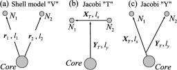
FIG. 3. Single-particle coordinate systems: ~a! ``V'' system typi- |
|
|
|
uY 5arctan |
|
|
|
|
Acore~Acore12 ! XY |
|
, |
|
|||||||||||||||||
|
|
|
|
|
|
|
|
|
|
|
|
|
|
|
|
|
|
|
|
|
|||||||||
|
|
|
FA |
~Acore11 !2 |
|
|
|
Y Y G |
|
||||||||||||||||||||
cal for a shell model. In the Jacobi ``T'' system ~b!, ``diproton'' and |
|
|
|
r |
|
|
|
|
|
|
|
|
|
||||||||||||||||
core are explicitly in con®gurations with de®nite angular momenta |
|
|
|
|
|
|
|
Acore |
|
|
|
|
Acore11 |
|
|
|
|
||||||||||||
lx and ly . For a heavy core the Jacobi ``Y '' system ~c! is close to the |
|
|
|
|
|
|
|
|
|
|
|
|
|
|
|
||||||||||||||
single-particle system ~a!. |
|
|
|
|
r |
25 |
|
|
|
|
|
XY2 1 |
|
|
|
|
|
Y Y2 . |
|
|
|
||||||||
|
|
|
|
|
|
|
|
|
|
|
|
|
|
|
|
||||||||||||||
|
|
|
|
|
|
|
Acore11 |
|
|
Acore12 |
|
|
|
|
|||||||||||||||
of lifetime connected with two-proton radioactivity. On the |
The wave functions ~WF! in this method is expanded over |
||||||||||||||||||||||||||||
the hyperspherical harmonics |
|
|
|
|
|
|
|
|
|
|
|
|
|
|
|
||||||||||||||
other hand the experimental techniques used with the radio- |
|
|
|
|
|
|
|
|
|
|
|
|
|
|
|
||||||||||||||
|
|
|
|
|
|
|
|
|
|
|
|
|
|
|
|
|
|
|
|
|
|
|
|
|
|
|
|
||
active nuclear beams put a lower limit on the practically |
|
|
|
|
|
|
|
|
|
|
|
|
|
1 |
|
|
|
|
|
|
|
|
|
|
|
|
|
|
|
detectable lifetime. 48Ni nucleus has been recently discov- |
C~X,Y!5C~r,Vr !5 |
|
( xKg~r! |
J |
Kg~Vr !, ~1! |
||||||||||||||||||||||||
ered @48#, with just the fact of the discovery putting an upper |
|
|
|
|
|
|
|
|
|
|
|
|
|
r5/2 |
Kg |
|
|
|
|
|
|
|
|
|
|
|
|||
limit on the energy of this nucleus ~Ref. @48#, see also the |
where JKg(Vr) is a set of orthonormal basis functions com- |
||||||||||||||||||||||||||||
discussion in Ref. @13#!. |
|||||||||||||||||||||||||||||
There exists widespread confusion about the nature of the |
plete on the hypersphere Vr5$ur ,VX ,VY % of ®xed radius |
||||||||||||||||||||||||||||
r. The hypermoment K is a generalized angular momentum, |
|||||||||||||||||||||||||||||
three-body decay ~two-proton radioactivity!, and which kind |
|||||||||||||||||||||||||||||
while the multi-index g stand for the rest of the quantum |
|||||||||||||||||||||||||||||
of experimental response should be expected. For us, three- |
|||||||||||||||||||||||||||||
numbers: total angular momentum L, angular momenta lx |
|||||||||||||||||||||||||||||
body decay is ®rst of all a true three-body process, requiring |
|||||||||||||||||||||||||||||
and l y associated with coordinates X and Y, total spin S, and |
|||||||||||||||||||||||||||||
genuine three-body dynamics for the understanding. The pro- |
|||||||||||||||||||||||||||||
spin Sx of the ``X'' subsystem. There are limits on the lowest |
|||||||||||||||||||||||||||||
cesses involving decays via narrow intermediate states could |
|||||||||||||||||||||||||||||
possible value of K, as K5lx1l y 12n; |
|
n50,1, . . . . Thus |
|||||||||||||||||||||||||||
be understood on the basis of two-body sequential models, |
|
||||||||||||||||||||||||||||
the states with nonzero total orbital angular momentum can- |
|||||||||||||||||||||||||||||
and do not belong to this class. The experimental ®ngerprint |
|||||||||||||||||||||||||||||
not be in the state with lowest hyperspherical excitation K |
|||||||||||||||||||||||||||||
of such true three-body process, as we tried to demonstrate in |
|||||||||||||||||||||||||||||
50. On the hyperspherical basis the variational procedure |
|||||||||||||||||||||||||||||
Ref. @13#, could be broad single particle and correlation spec- |
|||||||||||||||||||||||||||||
|
|
|
|
|
È |
|
|
|
|
|
|
|
|
|
|
|
|
|
|
|
|
|
|
|
|
|
|
||
tra. Other evidence for the process is an unexpectedly narrow |
reduces the Schrodinger equation to a set of coupled ordinary |
||||||||||||||||||||||||||||
differential equations: |
|
|
|
|
|
|
|
|
|
|
|
|
|
|
|
|
|
|
|
||||||||||
width. This is ordinarily connected with a strong suppression |
|
|
|
|
|
|
|
|
|
|
|
|
|
|
|
|
|
|
|
||||||||||
F |
|
|
|
|
|
|
|
|
|
|
|
|
$E2VKg,Kg~r!%GxKg~r! |
||||||||||||||||
of the three-body phase volume for small decay energies |
d |
2 |
|
L~L11 ! |
12 M |
||||||||||||||||||||||||
compared with the two-body one. |
|
2 |
|||||||||||||||||||||||||||
dr2 |
|
r2 |
|||||||||||||||||||||||||||
Below, we give a careful account of different qualitative |
|
|
|
|
|
|
|
|
|
|
|
|
|
|
|
|
|
|
|
|
|
|
|
|
|
|
|
|
|
approaches to the three-body decay problem and show their |
|
5 ( 2 M VKg,K8g8~r!xK8g8~r!, |
|
|
|
~2! |
|||||||||||||||||||||||
connection with the three-body calculations. We will see that |
|
|
|
|
|||||||||||||||||||||||||
often the qualitative approach successfully mimics the results |
|
|
|
K8g8 |
E |
|
|
|
|
J |
|
|
|
|
Fi. j |
|
|
|
|
|
|
GJ |
|
||||||
of the more precise approach. However, more care than usual |
|
|
|
|
|
|
|
|
|
|
|
|
|
|
|
|
|
|
|
|
|||||||||
|
|
|
|
|
|
|
|
|
|
|
² |
|
|
|
à |
|
~ri j ! |
|
|
|
|||||||||
is required in applying simple estimates for the three-body |
VKg,K8g8~r!5 |
|
dVr |
|
|
|
|
|
|
|
K8g8~Vr !, |
||||||||||||||||||
|
|
Kg |
~Vr ! ( V |
|
|
||||||||||||||||||||||||
decays. |
|
|
|
|
|
|
|
|
|
|
|
|
|
|
|
|
|
|
|
|
|
|
|
|
|
|
|
|
|
|
where E is the energy relative to the three-body threshold, M |
||||||||||||||||||||||||||||
B. NotationÐHyperspherical method |
is a ``scaling'' nucleon mass, and L5K13/2. |
|
|
|
|||||||||||||||||||||||||
|
The unit system \5c51 is used in the paper. When we |
||||||||||||||||||||||||||||
A detailed description of the HH formalism widely |
are not discussing experimental data, E is the energy relative |
||||||||||||||||||||||||||||
to the breakup threshold; sometimes another notation is used |
|||||||||||||||||||||||||||||
used for three-body bound states and continuum calculations |
|||||||||||||||||||||||||||||
for clarity E5ET5Q2 p52S2 p @see Fig. 1~a!#. The energy |
|||||||||||||||||||||||||||||
can be found elsewhere ~for example @49,12#!. Here we give |
|||||||||||||||||||||||||||||
only notations required in the context of this paper and only |
of the resonance in the core1p subsystem is expressed as |
||||||||||||||||||||||||||||
ER5S p2S2 p5S p1ET in terms of the separation energies. |
|||||||||||||||||||||||||||||
for systems like core1p1p. However, the generalization of |
|||||||||||||||||||||||||||||
the method for the other three-body systems is straightfor- |
|
|
|
|
|
II. ON THE POSSIBILITY |
|
|
|
|
|||||||||||||||||||
ward. |
|
|
|
|
|
|
|
|
|
||||||||||||||||||||
|
|
|
OF QUASICLASSICAL ESTIMATES |
|
|||||||||||||||||||||||||
In the HH method, the lengths of Jacobi vectors X and Y |
|
|
|
|
|||||||||||||||||||||||||
|
|
|
|
|
|
|
|
|
|
|
|
|
|
|
|
|
|
|
|
|
|
|
|
|
|
|
|
||
for three particles @Fig. 3~b!# are expressed via a hyperangle |
The enormous success of the Gamow's theory of radioac- |
||||||||||||||||||||||||||||
ur and a permutationally invariant hyper-radius r ~so its |
tivity was a demonstration of how a simple quasiclassical |
||||||||||||||||||||||||||||
value is the same in the systems Figs. 3~b!, ~c!. In the ``T'' |
formula can elucidate a wide class of physical processes. In |
||||||||||||||||||||||||||||
and ``Y '' systems they are |
this section we try to demonstrate that the attempts to ®nd an |
||||||||||||||||||||||||||||
054002-4
TWO-PROTON RADIOACTIVITY AND THREE-BODY . . .
adequate quasiclassical description of three-body decay processes must fail, and that a more complete few-body theory is required.
In simple estimates of three-body decays, three possible ``mechanisms'' are ordinarily discussed. Each of these decay mechanisms is associated with one of the coordinate systems in Fig. 3, by assuming that it is sensible to factorize the decay amplitudes in this particular system.
~i! Sequential emission mechanism @see Fig. 3~c!# assumes that ®rst the proton on Y axis is emitted, while the X subsystem core1p forms the long-living state. It is clearly adequate in the case of narrow intermediate states. However, the formalism is often applied even if there are no energy accessible states in the core1p system ~a condition of the ``true'' three-body decay!. Then the decay is considered via ``tails'' of Breit-Wigner amplitudes for the higher states @dotted arrows in Fig. 1~a!#, which are not well de®ned away from the resonance and thus do not have a precise physical meaning.
~ii! Qualitatively the idea of diproton radioactivity @Fig. 3~b!# is, that, due to the pairing, the two protons form a bosonic quasiparticle under the Coulomb barrier, which facilitates the penetration of the barrier. We will see below that, if improperly applied, this model can give a very misleading idea about two-proton radioactivity.
~iii! Simultaneous emission mechanism @Fig. 3~a!# is sometimes called ``direct decay to the continuum.'' This assumption seems to be well suited for heavier systems with strong Coulomb repulsion, where the interaction between protons is relatively small compared with a large core-p Coulomb interaction.
In the original paper of Goldansky the independent emission of two protons was assumed and the probability to penetrate via states with a de®nite distribution of energy between protons was estimated as the product of two independent penetrabilities
dW~uk ! |
6 |
|
|
|
|
|
52 |
|
|
sin uk cos uk |
|
|
prc3 M r3/2edET1/2 |
|
|||
duk |
|
|
|||
|
3Pl~ET sin2uk ,Zcore ,rc ! |
|
|||
|
3Pl~ET cos2uk ,Zcore ,rc !, |
~3! |
|||
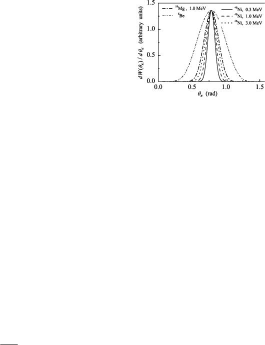
where uk5arctan@AEx /E y # is hyperangle in momentum space, the variable governing the energy distribution between the subsystems, and M red is a reduced mass in the core-p subsystem. The coef®cient in front of the penetrabilities plays the role of a reduced width and is normalized in the spirit of the Wigner limit: without any barriers the width is the average inverse ¯ight time for the distance rc/3. The
typical distributions estimated by Eq. ~3! are shown in Fig. 4 for 6Be ( p-shell nucleus!, 19Mg (d shell!, and 48Ni ( f shell!
at different energies. We have seen in Ref. @13# that there is a qualitative agreement between these estimates and the results of three-body calculations. The distributions in the Jacobi ``Y '' coordinate system ~which is close to ``V'' system for nuclei with heavy core! are always narrow and very
PHYSICAL REVIEW C 64 054002
FIG. 4. Estimated distribution of energy between protons according to Eq. ~3!. Solid, dashed, and dotted curves correspond to 48Ni with energies above threshold of 0.3, 1, and 3 MeV, respectively. Dash-dotted curve and dash-double-dotted curves correspond to 19Mg at 1 MeV and 6Be 01 with an experimental decay energy of 1.37 MeV.
similar independently of how the protons are correlated in the ``T'' system. So, this aspect of Goldansky's idea is con- ®rmed by the three-body calculations.
A. Problems of the diproton model
There are two technical observations that are probably responsible for the most widespread idea about the nature of two-proton radioactivity.
~i! It was noticed in the original paper @2# by Goldansky that, for estimates, it is suf®cient to approximate the decay width obtained from Eq. ~3! by the value obtained for equal energies of protons E15E2 (uk5p/4), because the distribution has a sharp peak there, as seen in Fig. 4. The two-proton width can then be estimated as
G}Pl2~ET/2,Zcore ,rch !. |
~4! |
In the case of l50, this expression is equivalent ~within an order of magnitude! to the expression for the penetration of a ``diproton'' ~particle with charge 2 but carrying all the energy of the system!,
G}Pl50~ET,2Zcore ,rch !. |
~5! |
The limits of applicability of such interpretation has been discussed in Refs. @2,5#. It should be noted that the original paper @2# is cautious about this simple ``diproton'' interpretation. From the fact that the penetrability of the s-wave barrier for a particle of mass 2, charge 2 with energy ET is approximately equal to product of s-wave penetrabilities of two particles of mass 1, charge 1, with equal energies ET/2, Goldansky draws the conclusion that ``the breakup of the sub-barrier diproton does not change the permeability if no additional interactions ~such as Coulomb repulsion! between two protons are considered.'' What he really considers to be a genuine signal of two-proton emission is ``energy correlation between the two protons, during the two-proton decay, which leads to their energies being almost equal'' in accor-
054002-5
GRIGORENKO, JOHNSON, MUKHA, THOMPSON, AND ZHUKOV |
PHYSICAL REVIEW C 64 054002 |
dance with Eq. ~4!. We have seen in Ref. @13# that the above estimates ~4! and ~5! correspond well to the results of dynamic calculations.
~ii! Let us assume some system with the two last ``valence'' nucleons in the same single shell and coupled to Jp
501. If we convert the valence nucleons WF from singleparticle coordinates @Fig. 3~a!# to the Jacobi ``T-system'' @Fig. 3~b!#, then, in the lowest shell-model approximation for j 5l 11/2 states, we get a large component with S50, lx
5ly 50: 66, 53, and 46 % for p-, d-, and f-shell population, respectively. Dynamically this con®guration should be even more enhanced by pairing and can be interpreted as a ``dipro-
ton'' (S50,lx50) in s-wave relative motion to the core. The considerations ~i! and ~ii! are probably responsible
for the manner in which the diproton model is ordinarily applied. For example, in papers @41,48# expression ~5! is used for p f -shell nuclei ~in paper @44#, a WKB approximation is employed, but essentially in the same way!. There are two reasons why this method of estimating may be inconsistent.
~i! The existence of such ``diproton'' in an s wave ``relative to the core'' is sometimes considered as opportunity to estimate penetration using s-wave penetrability expression for ``diproton'' particle as a whole. It is incorrect because, in spite of the recoupling of quantum numbers, the individual protons are still in a high-l state relative to the core.
~ii! The other problem with the ``diproton'' model is that two-proton correlation is not pointlike, and does not have zero internal energy. Applied as discussed above, the Eq. ~5! combines two incompatible things: penetration of a pointlike particle along some trajectory as well as zero relative motion energy for the constituents of this particle, which implies in®nite size due to the uncertainty principle. Strictly speaking the emission of the two particles with exactly zero relative energy has exactly zero phase volume ~and hence zero probability!.
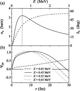
Unlike the n-n system that has a virtual state, the p-p
system forms a ``real'' resonance. The simple s-wave NN potential U(r)5231 exp@2(r/1.8)2#, used in this paper and in Ref. @13#, gives for a ``diproton'' the properties shown in Fig. 5. The elastic cross section has a peak at about E 50.55 MeV, but WF is only slightly enhanced in the internal region @Fig. 5~b!#. Of course, ``in the nuclear medium'' the diproton correlation should shrink, but the pictures shown in Fig. 5 provide a qualitative estimate of the range of the correlation. This corresponds well to the size of the penetrating two-proton correlation found in Ref. @13# ~see Fig. 4 there!.
Despite the criticism expressed about the traditional attitude to the diproton model, the simple estimates of Eqs. ~4! and ~5! are very useful. They provide, respectively, the lower and the upper limits for the width. This was con®rmed by the three-body calculations in Ref. @13#.
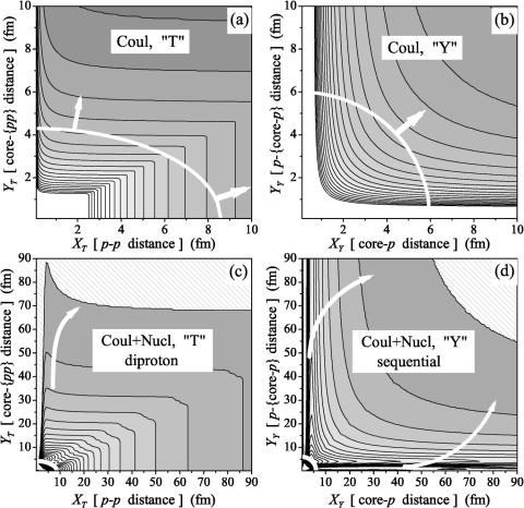
B.Potential surfaces
FIG. 5. ~a! Proton-proton elastic cross section ~solid curve! and phase shift ~dashed curve! for l50. ~b! WF for p-p relative motion at a low energy and for energies around the ``resonance.''
Let us consider 0 1 states, and only the WF's components in the lowest excitation. This mean @0s1/2#2 population in shell-model language, or a pure K50 WF component @see Eq. ~1!# in hyperspherical terms. This assumption might seem strange, as we are going to deal with systems where protons populate predominantly p-, d-, or f-shell states. However, calculations show that the partial decay width for the K50 component is much greater than for the others. The coupling to this WF component of the components dominating in the interior could be small, but the centrifugal barrier ~2! is the lowest for K50. So, by studying the potentials for this component, we get an idea about penetration for the system in general.
The Coulomb interaction of three particles depend on three variables ~say, interparticle distances ri j ). To visualize the potential surfaces we need to integrate over one of the variables. We can average over one variable in a way consistent with diproton or sequential emission models: by averaging over the angle uXY between vectors X and Y in ``T'' and ``Y '' systems, respectively,
|
a |
aZcore |
|
aZcore |
|
|||||
Vdi pr~X,Y !5 K |
|
1 |
|
|
|
1 |
|
L |
|
|
X |
uY1X/2u |
uY2X/2u |
|
|||||||
|
|
|
|
|
|
|
|
|
u |
XY |
Vseq~X,Y !5 K |
aZcore |
aZcore |
|
|||||||
|
|
|
1 |
|
|
|
||||
|
X |
|
uY2X/~Acore11 !u |
|
||||||
|
a |
|
|
1 |
|
L . ~6! |
|
uY1AcoreX/~Acore11 !u |
|||
|
|
u |
XY |
|
|
|
|
We have seen that the uncertainties of the diproton model are connected mainly with the ®nite size of the ``diproton'' particle. Can we provide a more accurate quasiclassical model that accounts for this?
The resulting potential surfaces are shown in Figs. 6~a!,~b! for one of the heaviest (48Ni) systems under consideration. The standard prescription of two-body R-matrix phenomenology is to ignore the interior, where the nuclear interac-
054002-6
TWO-PROTON RADIOACTIVITY AND THREE-BODY . . .
tion is strong and look for the lowest ``valley,'' suitable for penetration. Our experience with the three-body calculations shows that, in the absence of very strong correlations in the system ~e.g., bound states in the subsystems!, the surface r 5const is a good boundary for the interior of the system. This boundary is shown by elliptic curve in Fig. 6.
Studying the Figs. 6~a!,~b! we can ®nd that penetration paths contradict the assumptions, under which the corresponding plots were obtained. For Fig. 6~a!, supposed to be consistent with diproton model, the lowest valley ~shown by the thick arrow! is directed along values Y ;0 to large values of X ~protons ¯y out in opposite directions!. On the other hand, the sequential model Fig. 6~b! shows the deepest valley along the direction X'Y , where there is a signi®cant probability for two protons to be close to each other.
The reason for strange conclusions from Figs. 6~a!,~b! is the absence of nuclear interactions. Figures 6~c!,~d! show the deep moats that are dug in the potential surfaces Figs. 6~a!,~b! by a typical short-range nuclear potentials. On one hand it is clear that ribbons of classically allowed regions connecting the nuclear interior with the asymptotic region would facilitate the decay. On the other hand, the ``diproton valley'' in Fig. 6~c!, which is directly connected with the classically allowed region, should bring the system to free motion more quickly than the ``sequential valleys'' @in vicinity of XY 50 or Y Y 50 in Fig. 6~d!#, which are effectively dead ends. However, the valley Fig. 6~c! is too narrow for
PHYSICAL REVIEW C 64 054002
FIG. 6. Potential surfaces averaged over angle between X and Y for the component with lx5ly 50. ~a! and ~b! correspond to Coulomb potential for 48Ni in ``T'' and ``Y '' systems. ~c! and ~d! give the same plus nuclear potentials. The classically allowed region for E51.12 MeV is hatched in ~c! and ~d!. Elliptic curves correspond to surfaces r 56 fm. The arrows show most probable directions of penetration.
such a dispersed structure as a free diproton ~see Fig. 5!. So, moving along this lane the diproton will be hindered by ``spending a lot of time'' in a classically forbidden region, making it dif®cult to account for such decay mechanisms without proper dynamical treatment.
Our conclusion is that even in the simple case considered ~no channel coupling, etc.!, it is dif®cult to choose the quasiclassical path for decay of the three-body system properly. This means that with a simple expression for action along the path, there is no easy way to take into account the peculiarities of the three-body dynamics important for penetration.
III. THREE-BODY MODELS
A. Integral formula
It is clearly impractical to solve the scattering problem to ®nd the width of an extremely narrow state. To estimate the width of narrow two-body resonances, the integral method @50# was developed, based on the properties of the WF close to the S-matrix pole. Similar formulations can be found elsewhere in the literature @51#. It was used also in Ref. @12# under the name of ``generalized Feschbach method,'' however without much discussion. We found the application of the method in the three-body case nontrivial and deserving more attention. In the two-body case the method gives for the width
054002-7
GRIGORENKO, JOHNSON, MUKHA, THOMPSON, AND ZHUKOV PHYSICAL REVIEW C 64 054002
|
v U |
0 |
F |
|
r G |
U |
|
||
|
4 |
|
Ermaxdr |
|
|
vh |
|
2 |
|
G5 |
|
Fl~h,kr ! |
V~r !2 |
wl~r ! |
|
, ~7! |
|||
|
|
|
|
||||||
where v5k/ M red is the asymptotic velocity, h5Z1Z2a/v is the Sommerfeld parameter, Fl(h,kr) and Gl(h,kr) are Coulomb functions regular and irregular at the origin. The function wl(r) is a normalized ``box'' eigenfunction with quasiresonant boundary condition at large radius rmax
|
à |
k2 |
|
|
rmax |
2 |
|
F |
Tl1V~r !2 |
2 M red G |
wl~r !50, E |
|
druwl~r !u |
51, |
|
|
0 |
|
|
||||
~8!
1 |
|
|
||
wl~0 !50, wl~r !ur.rmax5 |
|
|
Gl~h,kr !, |
~9! |
A |
|
|||
N |
||||
Ã
where Tl is the kinetic energy for angular momentum l. The value N is a constant, which, under the normalization condition of Eq. ~8!, has the physical meaning of the ``number of particles'' inside the sphere radius rmax for unit outgoing current. For a narrow resonance, the second boundary condition in Eq. ~9! can be with a good precision replaced with simpler condition wl(rbox)50, where rbox may differ in general from the rmax . Reasonable values of rbox should be close to the outer classical turning point for the total potential.
Before we generalize the formula to the three-body case, the following issue should be discussed. Using the SchroÈdinger equation and then applying Green's theorem, Eq. ~7! could be rewritten as
G5 Uv4 2 M1red Wr„Fl~h,kr !,wl~r !…ur5rmaxU2, ~10!
for Wronskian Wr . Using the condition in Eq. ~9! this can be easily reduced to evident equality G5v/N: the width is a current through the sphere radius rmax divided by the number of particles inside it. This expression for the width comes out of exponential decay law N5N0 exp@2Gt#, and is valid if the width is small enough, so that the time dependent WF can be well parametrized as
wl~r,t !5e2Gt/22iEtwl~r ! |
~11! |
within the ®nite size domain @0,r
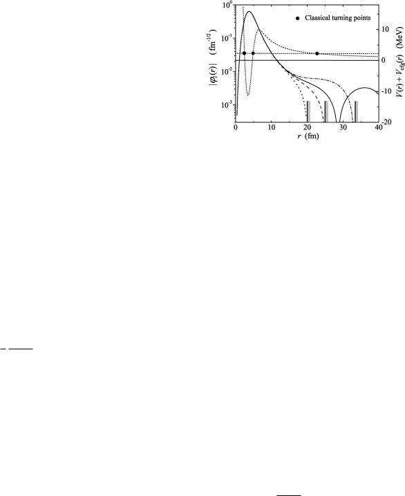
It is clear from Eq. ~10! that in the general case the width calculated by Eq. ~7! should be sensitive to the properties of wl at rmax . However, Fig. 7 shows that for narrow states formula ~7! can be practically applicable even if the WF wl(r) is obtained without special attention to the rmax boundary condition. It is clear from Fig. 7 that if we take rmax about 7±10 fm to the left of the outer classical turning point, the result would be insensitive to the ``box radius'' rbox taken in a wide range. This is due to the recovery of the correct behavior of the WF in the sub-barrier region. However, such a recovery depends on the numerical method used and the particular parameters of the problem, so de®nite caution is required in application of Eq. ~7!.
FIG. 7. Left axis: WF wl(r) calculated with quasiresonant boundary condition ~solid curve! and with ``box'' boundary condition with rbox520, 25, and 33 fm ~dotted, dashed, and dash-dotted curves!. The potential used in the calculation ~including the centrifugal term Vc f g) is shown opposite the right axis by the shortdashed curve and resonance energy is given by horizontal line of the same style. The state is 46Fe1p with l53, E52.276 MeV, and G50.1 keV ~subsystem for 48Ni at 1.12 MeV!.
In formal terms, the difference between the quasiresonant curve and those for ``box'' WFs in Fig. 7 is an admixture of the regular Coulomb function Fl . Since the quasiresonant solution matches exactly the function Gl , the relative contribution of the regular function Fl to the WF wl(r) decreases rapidly with decreasing radius under a strong Coulomb barrier. If this decrease is rapid enough, the function Fl does not in¯uence the solution in the nuclear interior. Then, as far as the regular function admixture does not contribute to the Wronskian in Eq. ~10!, the formula ~7! should work well.
Using the hyperspherical expansion, the formula ~7! can be generalized to the three-body case. However, due to the fact that three-body Coulomb asymptotic state is unknown, it can be done only with some approximations, which are discussed below in Sec. III C. The three-body width is given by
4 |
( ( E |
rmax |
(R) |
|
|
||
G5 |
|
|
dr xKg,K8g8 |
~r! |
|
||
|
|
|
|||||
v |
Kg UK8g8,K9g9 0 |
|
|
|
|
||
|
|
|
|
|
|
|
2 |
|
|
|
subt |
|
box |
~r!U , |
|
3@VK8g8,K9g9~r!2VK8g8,K9g9 |
~r!#xK9g9 |
||||||
~12!
where v5k/ M , k5A2 M ET, and M is nucleon mass. Functions xbKogx(r) are the hyperspherical components of the ``box'' WF having positive energy,
à |
~13! |
~H2Ebox !Cbox~r,Vr !50, |
calculated in the bounded domain @0,rbox # with zero boundary conditions at both sides. Practically, the value rbox should be as large as possible, but still in the classically forbidden region. Potentials V and functions x
de®ned in Sec. III C for different approximate boundary conditions.
054002-8
TWO-PROTON RADIOACTIVITY AND THREE-BODY . . .
This formalism has been applied in Ref. @12# to the continuum states of A56 nuclei and compared with 3!3 resonance scattering. The model has some disadvantages. First of all in the three-body problem it can be dif®cult to bring the ``box'' solution out far enough in the r direction. We will see later that for low energies above threshold and strong Coulomb potentials, it can lead to serious underestimation of the decay width. Also, for energies close to the top barrier the signi®cant imaginary part in energy ~and hence in k) is not taken properly into account in Eq. ~12!. There exists a generalization of Eq. ~7! for wide resonances @52#, but we do not think it is worth incorporating in our three-body cases with small G.
B. Model with a source
A more robust and transparent model can be built as follows. Suppose that the positive energy state was populated by some process, and in a while it decays. Such a situation is described by a time-dependent WF C(1)(r,Vr ,t) with purely outgoing asymptotics. For narrow resonances this WF in a ®nite size domain can be parametrized as
C(1)~r,Vr ,t !5exp~2G/2t2iEt !C(1)~r,Vr !
with a great precision, and the time-independent part should satisfy the SchroÈdinger equation
à |
(1) |
~r,Vr !50. |
~14! |
~H2E1iG/2!C |
|
This equation is solved approximately using the intuitive idea that for very narrow state the WF should be very close to the ``box'' WF Cbox of Eq. ~13!. The WF Cbox is then used as a source term to derive the WF with outgoing asymptotic waves
à |
(1) |
~r,Vr !52iG/2Cbox~r,Vr !. |
~15! |
~H2Ebox !C |
|
The system is solved with boundary condition of matching to
the purely outgoing functions x(1) (r) at r5rmax @see
Kg,K8g8
Eqs. ~19!, ~21!, and ~22! for details of different approximations#. The equation ~15! is ®rst solved with arbitrary constant G/2 and to de®ne the value of width G the following expression is used:
1 |
|
Im E dVrC(1)²r5/2~d/dr!r5/2C(1)urbox |
|||
G5 |
|
|
|
|
. ~16! |
|
|
r |
|
||
|
M |
|
E dVr E0 |
maxdr r5uC(1)u2 |
|
This formula can be rigorously obtained for rbox5rmax by applying the Green's theorem to the SchroÈdinger equation. It has a simple physical meaning similar to what we have seen for Eq. ~11!: for systems obeying the exponential decay law, the width is the ratio of current through a hypersphere of large radius to number of particles inside it. For narrow reso-
PHYSICAL REVIEW C 64 054002
nances there is no practical necessity to keep rbox5rmax because the WF practically vanishes under the barrier. However it can be sensible to keep them different (rbox,rmax) for the case of wide states, as it will be discussed in the end of this section.
Some remarks should be made about the source model. ~i! The model could be considered as the ®rst step in an iterative method of solving Eq. ~14!. It is clear that even the ®rst iteration is suf®cient if the ratio uG/Eu is small enough. ~ii! At a ®rst glance the model method should not work for the wide (G.100 keV! nuclear states, because above the barrier the ``box'' WF becomes unstable with respect to the boundary conditions. In reality in such a situation the ®rst iteration may be more useful than the exact solution. The ®rst iteration could portray quite realistically how such a wide resonance may be populated in a nuclear reaction creating a compact initial con®guration which then decays ~the situation is typical for widely used experimental techniques, like missing mass measurements!.
C. Sensitivity to boundary conditions
When studying systems of nuclei and nucleons we face only a ``simple'' subset of the three-body Coulomb problem in the continuum: all the long-range interactions are repulsive and there is no problem with an in®nite number of states in subsystems as for the attractive Coulomb potentials. We simplify the task even more by considering only three-body systems that do not have bound subsystems. In this case the asymptotic form for all three interparticle distances tending to in®nity should be suf®cient. This form ~sometimes called ``Redmont-Merkuriev''! is analytically known ~see, for example, @53,54# and references therein!, but is quite complicated to implement. In this paper we use different approximate boundary conditions which mean that the Coulomb interaction is somehow distorted at large distances. However, we will show that if the region of dynamical calculation and the basis set are both large enough, then the energy, the width, and the WF in the ``internal'' domain can be obtained with suf®cient reliability.
The following approximate boundary conditions are used with the models described in the previous sections ~everywhere below, the summation over the repeating indices is implied!:
a. Plane wave. All the Coulomb potentials are set to zero at some large-radius rmax and Bessel-Rikatti functions corresponding to three-body plane wave are used in Eq. ~12!, with
subt |
|
|
hKg50; VKg,K8g8 |
~r!50. |
~17! |
b. Diagonal Coulomb potentials. A better approximation is to cut only the nondiagonal Coulomb potentials from some
large-radius rmax and use in Eq. ~12! the Coulomb functions of half-integer order with Sommerfeld parameter correspond-
ing to the ``effective charge'' in each hyperspherical channel K,g:
054002-9
GRIGORENKO, JOHNSON, MUKHA, THOMPSON, AND ZHUKOV |
PHYSICAL REVIEW C 64 054002 |
|||||||||
|
rmax |
Coul |
|
|
|
|
||||
hKg5 |
|
|
|
|
VKg,Kg~rmax!, |
|
|
|
||
v |
|
|
|
|||||||
|
|
|
|
|
|
|
||||
subt |
|
vhKg |
|
, |
~18! |
|
||||
VKg,K8g8 |
5 |
|
|
dKg,K8g8 |
|
|||||
r |
|
|||||||||
Coul
where VKg,K8g8 is Coulomb part of the three-body interactions @see Eq. ~2!#. If the charge distributions of the particles are taken into account, the rmax value should be large enough to get a constant value of hKg .
In both the cases mentioned above, the functions x should be taken as
x(R) |
5d |
Kg,K8g8 |
F |
~h |
Kg |
,kr!, |
~19! |
Kg,K8g8 |
|
|
L |
|
|
where L5K13/2.
c. Diagonalized Coulomb potentials. We can diagonalize the Coulomb coupling potentials on the ®xed hyperspherical
basis at rmax . For this case hKg and Vsubt entering Eq.
~12! are de®ned as
Kg,K8g
|
rmax |
T |
|
|
Coul |
|
~rmax!AK9g9,Kg , |
||||
hKg5 |
|
|
AKg,K8g8VK8g8,K9g9 |
||||||||
v |
|||||||||||
Vsubt |
|
52d |
Kg,K8g8 |
L~L11 ! |
1A |
Kg,K9g9 |
|||||
|
|
|
|||||||||
Kg,K8g8 |
|
|
|
|
r |
2 |
|
||||
|
|
3F |
|
|
|
|
|
GAKT 9g9,K8g8 , ~20! |
|||
|
|
vhK9g9 |
1 |
L0~L011 ! |
|||||||
|
|
r |
r2 |
||||||||
where the orthogonal matrix AKg,K8g8 diagonalizes the Cou-
à |
Coul à à à |
à |
|
lomb potential matrix: V |
A5Al, with l diagonal. In this |
||
case the functions x(R) are taken as |
|
|
|
(R) |
|
~hK8g8 ,kr! |
~21! |
xKg,K8g85AKg,K8g8FL0 |
|||
in Eq. ~12!. This diagonalization procedure removes the nondiagonal potentials behaving like r21. However, the centrifugal potentials are not diagonal any more and we end up with coupling interactions that decrease as r22. It is clear that this approximation will give the best results if the rmax value is large enough to make the centrifugal terms small compared with the energy, but not too large, so that the truncated hyperspherical basis is still adequate to the situation. We found that stable results are obtained if the index L0 is taken the same for all the channels in Eq. ~21!. The value of L05K013/2 is quite arbitrary and we demonstrate in Fig. 8c that the results for K050 ±4 are very stable and close to each other.
Functions x(1) @needed for solving Eqs. ~14! and ~15!# can be obtained from x(R) by substitution
FL!GL1iFL . ~22!
The Coulomb functions FL and GL in Eqs. ~19!, ~21!, and ~22! satisfy the decoupled hyperspherical equations ~2! with potentials
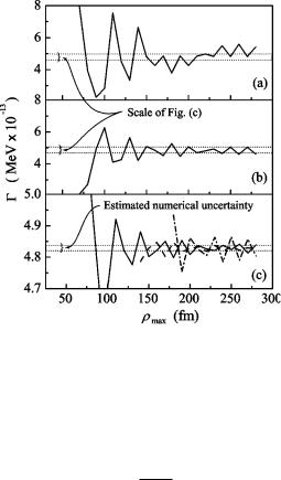
FIG. 8. The width as a function of matching radius rmax in the case of 48Ni at E52.09 MeV calculated with source model. Parts ~a!, ~b!, and ~c! correspond to the boundary conditions de®ned in a, b, and c, respectively. Solid, dashed, and dash-dotted curves in ~c! correspond to K050, 2, and 4. The range of ~c! is shown by dashed lines in ~a! and ~b!.
vhKg
VKg,K8g8~r!5 r dKg,K8g8 .
The results of calculations of the width G as a function of matching radius rmax for the 48Ni case using the source model with different boundary conditions are shown in Fig. 8. The important thing is that all the approximations give the same result ``on average.'' It is clear that all types of approximations work best after a certain hyper-radial range of dynamic calculation is achieved ~it is about 150 fm for Fig. 8!. Even the most crude approximation with outgoing plane wave @Fig. 8~a!# has less than 25% instability. The instability of calculations with diagonalized Coulomb interactions shown in Fig. 8~c! is much less than in the other models and seems to be purely numerical ~it can be estimated independently to be at the level of 0.5% in this particular case!.
Figure 8 also allows us to draw a conclusion about applicability of the integral formula Eq. ~12!. Models should give
the same results for rmax5rbox . To stabilize the width we need to take rmax about 150 fm. However, we cannot make
the box size rbox more than 60±70 fm due to appearance of the spurious solutions with a too large probability outside the barrier. It is clear from Fig. 8 that in such case the result of the integral formula cannot be better than an order of magnitude estimate.
The last thing we need to demonstrate is the sensitivity of calculations to the box size rbox . Figure 9 shows that sensible results can be obtained for the box as small as 12±15 fm. For boundary conditions given by Eqs. ~17! and ~18! the choice of this parameter impose signi®cant uncertainty, while for diagonalized Coulomb potential boundary conditions of
054002-10